APPLICATION OF SCADA DATA MONITORING METHODOLOGY AND RELIABILITY ANALYSIS OF WIND FARM OPERATIONAL DATA
Dissertation in partial fulfillment of the requirements for the degree of
MASTER OF SCIENCE WITH A MAJOR IN ENERGY TECHNOLOGY WITH FOCUS ON WIND POWER
Uppsala University
Department of Earth Sciences, Campus Gotland
Bojan Alavanja
APPLICATION OF SCADA DATA MONITORING METHODOLOGY AND RELIABILITY ANALYSIS OF WIND FARM OPERATIONAL DATA
Dissertation in partial fulfillment of the requirements for the degree of
MASTER OF SCIENCE WITH A MAJOR IN ENERGY TECHNOLOGY WITH FOCUS ON WIND POWER
Uppsala University
Department of Earth Sciences, Campus Gotland
Approved by:
Supervisor, Prof. Jens N. Sørensen
Examiner, Prof. Simon-Philippe Breton
ABSTRACT
Reliability of wind turbine components and maintenance optimisation are among the critical aspects of wind power development closely related to profitability and future development. The main reason for research in these areas is lowering the cost of energy production for wind power, specifically important in offshore environment. Continuous monitoring of specific wind turbine components can be valuable for wind farm operators and, subsequently, wind farm owners. Also, health assessment of critical components can be useful in estimating the possibilities for life extension of wind turbines. Expensive Condition Monitoring Systems (CMSs) are not always available, particularly in older wind farms, and additionally installing CMSs on wind turbines is not always economically feasible. However, most of modern wind turbines are equipped with the Supervisory Control And Data Acquisition (SCADA) system which is recording 10-minute average values of parameters that depict operation of the turbine. That being said, SCADA data contains a vast amount of information that can be used for analysis of wind turbine components health. Therefore, this project will present an application of previously published methodology for SCADA data condition monitoring on real wind farm data. The goal of this project is to investigate on the possibilities of the SCADA monitoring methodology and what can be the added value of the application for wind farm operators, owners and other stakeholders.
The methodology for condition monitoring through SCADA data was applied on real data gathered from two wind farms in Germany and one in the Netherlands. During the project the methodology had to be modified in order to ensure the best possible industrial application. Results of the project showed that the SCADA data condition monitoring approach is not capable of predicting failures. However, the technique has been proven successful for detecting the changes of trends in dependencies of working parameters, specifically monitoring parameters related to the turbine generators. Continuously monitoring the dependencies of working parameters can be used as an additional source of information for maintenance scheduling and assessment of components health. The approach presented in this paper can be valuable to asset managers and wind farm owners.
Key words: SCADA, condition monitoring, maintenance scheduling, wind turbine reliability, availability, life extension prediction
ACKNOWLEDGEMENTS
I would like to thank my supervisor professor Jens Nørkær Sørensen for his guidance throughout this project. I would also like to thank Ferdy Hengeveld who was my supervisor at Mecal Wind / Energy department for enabling me to do my project with real wind farm data and get a first hand experience in the wind power industry.
Special thanks goes to Harmen Links who is the Project Engineer at Mecal Wind / Energy department and whom helped me the most with his expertise, insightful advice and critical opinion. Thanks also go to my friends and colleagues that I met on my journey through Sweden and the Netherlands for making my past year an unforgettable experience.
Finally yet importantly, I want to thank my mother and father for their unconditional support, understanding and love. Hvala ti oče i hvala ti mati za sve što jesam i što ću ikad biti, dugujem vama.
NOMENCLATURE
CMS Condition Monitoring System
IA Information available
IAN Information available non operative category IAO Information available operative category
IAOG Information available operative generating category IAONG Information available operative non generating category
IAONGENC Information available operative non generating out of environmental specification optional category - calm winds
IAFM Information available force majeure category IEC International Electrotechnical Commission
IU Information unavailable
KPI Key Performance Indicator
LWK Landwirtschaftskammer Schleswig-Holstein (Chamber of Agriculture Schleswig-Holstein)
MTBF Mean Time Between Failures
MTTF Mean Time To Failure
MTTR Mean Time To Repair
N/A Not applicable
RPM Revolutions per minute
SCADA Supervisory Control And Data Acquisition
SQL Structured Query Language
T Turbine
WF Wind farm
WMEP Wissenschaftliches Mess und Evaluierungsprogramm (Scientific Measurement and Evaluation Programme)
Page
ABSTRACT ... iii
ACKNOWLEDGEMENTS ... iv
NOMENCLATURE ... v
TABLE OF CONTENTS ... vi
LIST OF FIGURES ... vii
LIST OF TABLES ... viii
CHAPTER 1. INTRODUCTION ... 1
CHAPTER 2. LITERATURE REVIEW ... 4
2.1 Introduction ... 4
2.2 Wind turbine availability ... 4
2.3 Wind turbine reliability ... 5
2.3.1 Failure intensity and reliability metrics ... 9
2.3.2 Environmental impact on wind turbine reliability and availability ... 11
2.4 SCADA data monitoring techniques ... 12
CHAPTER 3. METHODOLOGY AND DATA ... 13
3.1 Introduction ... 13
3.2 Input data ... 13
3.3 Data processing ... 14
3.3.1 Wind turbine taxonomy ... 14
3.3.2 Availability calculation ... 15
3.3.3 MTBF, MTTF & MTTR... 16
3.4 SCADA data monitoring application ... 17
3.4.1 Calculating the coefficient representing the state of the component ... 20
3.5 Continuous monitoring ... 22
3.5.1 Testing methodology and potential correlations ... 25
3.6 Results analysis ... 26
CHAPTER 4. APPLICATION OF THE METHODOLOGY AND RESULTS ... 27
4.1 Introduction ... 27
4.2 Downtime statistics ... 27
4.3 Generator monitoring ... 32
4.4 Gearbox monitoring ... 37
CHAPTER 5. DISCUSSION AND ANALYSIS ... 43
CHAPTER 6. CONCLUSIONS ... 45
REFERENCES ... 49
APPENDIX A ... 51
Page Figure 2.1 Distribution of failure rate and downtime by subassembly, reproduced from the
ReliaWind project, Source: Whittle, 2013 ... 6
Figure 2.2 Average rate of failure vs wind turbine components, Source: Pinar Pérez et al., 2013 ... 8
Figure 2.3 Distribution of failures by subassembly and categorised as either major or minor failures, Source: Faulstich, Hahn & Tavner, 2011 ... 8
Figure 2.4 The bathtub curve where β<1 represents a decreasing failure rate, β=1 represents a constant failure rate and β>1 represents an increasing failure rate, Source: Spinato et al., 2008 ... 9
Figure 2.5 Relation between the reliability metrics, Source: Tavner, 2009 ... 10
Figure 3.1 Methodological framework ... 13
Figure 3.2 Example generator speed and wind speed correlation extracted from SCADA data; blue and red dots and lines represent two different time periods a) plot of 10-minute values b) 10-minute values after binning ... 19
Figure 4.1 Failure occurrences and downtime statistics for the WF1 wind farm ... 27
Figure 4.2 Failure occurrences and downtime statistics for the WF2 wind farm ... 29
Figure 4.3 Failure occurrences and downtime statistics for the WF3 wind farm ... 30
Figure 4.4 Change of the 𝑐 coefficients for the WF1 wind farm without additional filtering; monitoring the correlation between generator speed and generator power ... 33
Figure 4.5 Change of the 𝑐 coefficients for the WF1 wind farm; monitoring the correlation between generator speed and generator power ... 34
Figure 4.6 Power curve change for the WF1 – T01 wind turbine; red and blue dots and lines represent periods before the 7th and after the 8th iteration, respectively a) 10-minute values b) binned power curve ... 35
Figure 4.7 Change of the 𝑐 coefficients for the WF1 wind farm with fixed historical data; monitoring the correlation between generator speed and generator power ... 36
Figure 4.8 Change of the 𝑐 coefficients for the WF2 wind farm; monitoring the correlation between rotor speed and gearbox temperature ... 37
Figure 4.9 Change of the 𝑐 coefficients for the WF2 wind farm with moving historical data; monitoring the correlation between rotor speed and gearbox temperature ... 39
Figure 4.10 Change of the 𝑐 coefficients for the WF3 wind farm; monitoring the correlation between rotor speed and gearbox temperature ... 40
Figure 4.11 Change of the 𝑐 coefficients for the WF3 wind farm with 20 partitions; monitoring the correlation between rotor speed and gearbox temperature ... 41
LIST OF TABLES
Page
Table 2.1 Failure statistics for critical components of wind turbines, reproduced from the ReliaWind project, Source: Bertling Tjernberg & Wennerhag, 2012 ... 7 Table 2.2 Reliability of generators, gearboxes and converters, Source: Spinato et al., 2008 10 Table 3.1 Example of the taxonomy used in ReliaWind, Source: Tavner, 2011 ... 15 Table 3.2 Illustration showing the additional filtering process. Only the data from
the periods when data is available for all of the turbines in the analysis
is to be used in the calculations, Source: Links, 2016 ... 24 Table 3.3 Statistics of available SCADA data after the filtering processes ... 24 Table 4.1 Availability, reliability and average values of parameters for the
WF1 wind farm ... 28 Table 4.2 Availability, reliability and average values of parameters for the
WF2 wind farm ... 29 Table 4.3 Availability, reliability and average values of parameters for the
WF3 wind farm ... 31 Table 4.4 Timestamps of the iterations in the WF1 wind farm example ... 35 Table 4.5 Turbine WF2 - T04 alarm log and gearbox related alarms
CHAPTER 1. INTRODUCTION
As the number of wind farms in the world is growing rapidly every year, new technologies are being developed and implemented in wind farm operation and maintenance. One of the most significant issues, and an area for improvement, is the reliability of operating wind farms. There are many published papers on wind turbine reliability and the current trend is leaning towards the use of Condition Monitoring Systems (CMSs). As wind power development is moving to even more remote locations and offshore environment, there is a need for reliable and effective condition monitoring techniques and systems. The state-of-the-art research is based on CMS applications which usually involve installation of additional sensors and devices for monitoring different operational parameters. However, a majority of modern wind turbines are already equipped with a variety of monitoring sensors that are part of the Supervisory Control And Data Acquisition (SCADA) system. The SCADA system is monitoring and recording different turbine parameters as 10-minute average values throughout the lifetime of a turbine. Aside from the SCADA system, turbine monitoring system is also archiving different alarm occurrences and downtimes in the alarm logs.
An extensive amount of research has been published about utilizing SCADA data for condition monitoring and health assessment of wind turbines. With that in mind, the goal of this thesis project is to implement an application for monitoring wind turbine components through SCADA data and answer several questions regarding wind turbine reliability. The questions that this paper will try to answer are:
Is the chosen SCADA data monitoring approach sufficient to predict failure of specific turbine components?
What are the main limitations for using SCADA data for condition monitoring?
How can SCADA data monitoring be used as a complementary tool in wind farm operation and maintenance?
The research will concentrate on the correlation between reliability of wind turbines, or specific parts of its assembly, and the Key Performance Indicators (KPIs) that can be extracted from the alarm logs and SCADA data. The KPIs in this case will represent the dependency between pairs of SCADA parameters. The investigation will be performed with the database that has been
provided by a Dutch company called MECAL and their Wind/Energy department. The available data consists of SCADA and alarm logs from two operating wind farms located in Germany and one in the Netherlands. During the analysis of wind turbines any additional information, like maintenance logs or purchase bills, are desirable. Unfortunately, this kind of information is not always available and the analysis can only be done with available SCADA and alarm logs. Therefore, with the data that is available, this project will apply a SCADA data condition monitoring methodology and assess its possibilities.
Thesis overview
Chapter 2 – Literature review
The literature review will present current statistics and findings regarding wind turbine reliability and the SCADA data condition monitoring techniques. A vast amount of statistics has been published on the topic of wind turbine reliability and downtime statistics, these will be used as reference for analysing the experimental wind farms. The purpose of this comparison is to validate the available datasets that are later on going to be used for the SCADA data condition monitoring.
Chapter 3 – Methodology and data
This chapter will present the calculation steps and monitoring approach with a detailed explanation of the methodology and the available datasets. The methodology starts with processing the alarm logs and SCADA data from a given wind farm, after which the SCADA monitoring technique can be applied. Also, this chapter will explain the reasoning behind the application process and the modifications made during the application.
Chapter 4 – Application of the methodology and results
The results from the application of the methodology on three available wind farm datasets will be presented in this chapter. Different cases will be presented for each one of the wind farms; the starting conditions for the calculations will differ in order to enable sensitivity analysis. With research ethics in mind, the examples will be chosen to best represent the monitoring approach, with all of the advantages and deficiencies.
Chapter 5 – Discussion and analysis
The results and findings will be discussed and analysed in this chapter. Main observations regarding the application process will be presented after which the accuracy and sensitivity will be discussed. Also, similar studies that were previously published will be mentioned and compared.
Chapter 6 – Conclusions
Main conclusions and summary of all of the findings will be presented in this chapter, together with possibilities for future work. Based on experience gained from the application process, a recommendation will be given on how to employ the SCADA data monitoring technique during wind farm operation and maintenance.
CHAPTER 2. LITERATURE REVIEW
2.1 Introduction
Statistical analysis of wind farm alarm logs can point out the most unreliable wind turbines and components that fail most often or cause the most downtime. Availability, reliability and reliability metrics of wind turbines and their components are the statistics that can be extracted from the alarm logs. Additionally, SCADA logs can be used for monitoring specific wind turbine parameters in order to detect changes in wind turbine performance and components condition. The approach for SCADA data monitoring that is going to be used in this paper is based on dependencies between a couple of parameters and their change over time. This approach is more complex than just monitoring one parameter and setting a threshold for an alarm. The literature review will present the research and statistics that have been previously published on wind turbine availability, reliability and SCADA data monitoring techniques and their application.
2.2 Wind turbine availability
For the purposes of this research the meaning of wind turbine availability has to be clearly defined. The availability of wind turbines can be interpreted and calculated in several different ways. The International Electrotechnical Commission (IEC) published the IEC/TS 61400-26-1 standard which specifies the terms for time based availability of a wind turbine generating system. In the IEC standard wind turbine availability has been defined as (The International Electrotechnical Commission, 2011):
“Availability - fraction of a given operating period in which a wind turbine generating system is performing its intended services within the design specification.”
Time based availability can either be operational availability or technical availability, both are widely used within the industry. Operational availability represents the wind turbine user’s view on availability and it is considering time periods when the wind turbine is actually generating. While the technical availability would be the manufacturer’s view on availability, considering time periods when the wind turbine is operating according to the design specifications. Operational availability is relatively simple to calculate and it can easily be extracted from the alarm logs and SCADA data. Technical availability requires more detailed information regarding the operation
of a wind turbine. Depending on the level of detail and quality of the SCADA data and alarm logs, technical availability sometimes cannot be correctly calculated without additional information. Therefore, operational availability will be calculated and used for comparison of wind turbines in this project, according to the standard it is defined as (The International Electrotechnical Commission, 2011):
“Operational availability - System operational availability is the fraction of a given period of time in which a wind turbine generating system is actually generating. Lost operating hours due to any reason are included as unavailability.”
The statistics regarding wind turbine availability were published from different sources in the past years. Based on statistics made with data from approximately 250 wind farms, 50 % of the almost 750 wind farm years combined reported technical availability greater than 97.5 %, while the same technical availability dropped below 90 % for only 6 % of the wind farm years. Moreover, for onshore wind turbines it is reasonable to expect 97 % availability on average, over the typical 20 years of lifetime (Harman, et al., 2008). However, this high rate of technical availability is due to frequent maintenance and not just good reliability of turbine components (Ribrant, 2006).
2.3 Wind turbine reliability
Wind turbine reliability has been defined in the IEC standards as (The International Electrotechnical Commission, 2011):
“Reliability - probability that a component part, equipment, or system will satisfactorily perform its intended function under given circumstances for a specified period of time”
Over the past few decades an extensive database of wind turbine reliability statistics has been collected and published. There are several papers that represent the failure statistics of wind turbines and their components. The statistics are mostly based on wind turbine populations in Germany, Denmark, Sweden and Finland. There are certain differences in the analysis approach and reporting method among the published statistics. Since the studies were conducted independently the data is presented in various ways, that can be failure or downtime distributions or failure rates presented per turbine or per year. However, the taxonomy of turbines in these
publications is similar and the location of the wind farms that were subject of the research is Northern Europe, same as the example wind farms in this project. These statistics will be reviewed and presented for comparison and validation of the data that is available from the MECAL database.
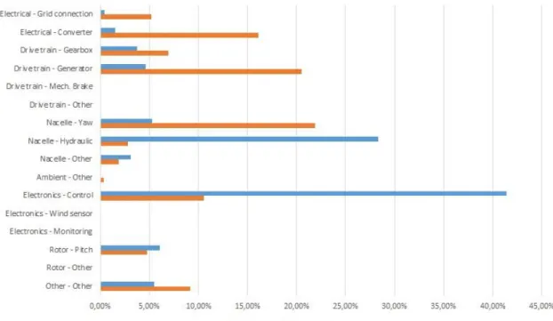
The Wissenschaftliches Mess und Evaluierungsprogramm (WMEP) was a German survey carried out from 1989. to 2006. and it included almost 1500 different turbines. The result from WMEP research was a detailed database containing the data regarding availability and reliability of wind turbines. Another valuable survey with similar results was the Landwirtschaftskammer Schleswig-Holstein (LWK), it was carried out from 1996. to 2006. and the survey analysed more than 650 turbines (Pettersson, et al., 2010). Results from the WMEP and LWK surveys were combined and additionally processed in the ReliaWind project. The ReliaWind project was carried out from 2008. until 2011. and it has produced a statistic of failure occurrences and downtime of wind turbines on a subassembly level, see Figure 2.1.
Figure 2.1 Distribution of failure rate and downtime by subassembly, reproduced from the ReliaWind project, Source: Whittle, 2013
Summary of the ReliaWind project presented as the failure statistics of the most critical wind turbine components, which cause the highest downtime and breakdown most frequently, can be seen in Table 2.1.
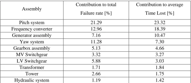
Table 2.1 Failure statistics for critical components of wind turbines, reproduced from the ReliaWind project, Source: Bertling Tjernberg & Wennerhag, 2012
Assembly Contribution to total Failure rate [%] Contribution to average Time Lost [%] Pitch system 21.29 23.32 Frequency converter 12.96 18.39 Generator assembly 7.16 10.47 Yaw system 11.28 7.30 Gearbox assembly 5.13 4.66 MV Switchgear 3.32 3.27 LV Switchgear 5.88 3.03 Transformer 1.71 1.84 Tower 2.66 1.75 Hydraulic system 1.19 1.42
From the statistics shown above, it is obvious that the highest failure contribution is originating in electrical system components like the electrical converter, generator and switchgears. Subsequently, pitch system which is a part of rotor module is the source of a great part of the downtime (Bertling Tjernberg & Wennerhag, 2012).
Recently, Pinar Pérez et al. (2013) published a comprehensive review and analysis of the major studies conducted on wind turbine reliability. The general observations regarding the topic are that even though the nomenclature is not exactly the same and the data is aggregated in the papers, for confidentiality reasons, the reported failure rates do not vary much between different studies. Gearboxes, generators and blades have been identified as the most critical parts as their failures lead to the longest downtimes. When it comes to failure rates most cited turbine parts are blades, electrics and control systems. The average failure rates for wind turbines are shown in Figure 2.2.
Figure 2.2 Average rate of failure vs wind turbine components, Source: Pinar Pérez et al., 2013
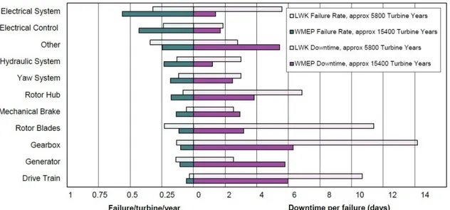
Similar statistics which show the annual failure rate as well as the average downtime per failure were published by Faulstich, Hahn & Tavner (2011), see Figure 2.3.
Figure 2.3 Distribution of failures by subassembly and categorised as either major or minor failures, Source: Faulstich, Hahn & Tavner, 2011
Another study showed that for onshore wind farms 75 % of failure occurrences caused only 5 % of downtime while the remaining 25 % of failures were the reason for remaining 95 % of downtime. Furthermore, within the 25 % of failures the predominant origins are gearbox, generator and drive train (Faulstich, et al., 2009).
2.3.1 Failure intensity and reliability metrics
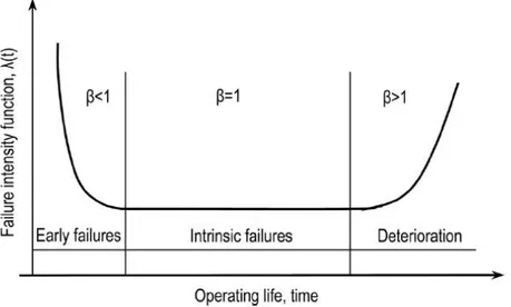
The reliability of repairable systems can be modelled with a bathtub curve which distinguishes three different stages of systems operational lifetime (Spinato, et al., 2008). The three stages are commonly labelled as the infant mortality, the normal and the wear-out stage of the bathtub curve, see Figure 2.4. The rationale behind these three stages is based on the fact that the failure rate of a system is initially very high, after the initial period the failure rate declines and stays stable until, after some time, the system starts to wear out and the failure rate increases again. Each of these stages can be modelled with a failure intensity function.
Figure 2.4 The bathtub curve where β<1 represents a decreasing failure rate, β=1 represents a constant failure rate and β>1 represents an increasing failure rate, Source: Spinato et al., 2008
When analysing wind farm data, it is important to determine in which stage of operating life are the turbines in the wind farm. During the analysis of wind farm alarm logs the reliability metrics can be of value to describe individual wind turbines and the wind farm. The reliability metrics are:
- Mean Time Between Failures (MTBF): The average time between two failures of the whole system, assembly or component (Barbati, 2009).
- Mean Time To Failure (MTTF): Very similar to MTBF, it represents the average time from repair to the following failure (Barbati, 2009).
- Mean Time To Repair (MTTR): Defines the average time until repair after the failure (Barbati, 2009).
The relation between the reliability metrics is shown in Figure 2.5
Figure 2.5 Relation between the reliability metrics, Source: Tavner, 2009
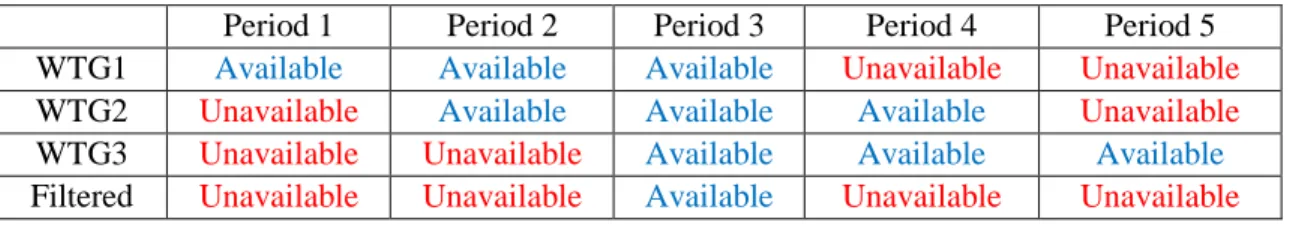
Reliability metrics are usually calculated for turbine components separately and the statistics found in literature can more closely describe the reliability of critical components, see Table 2.2.
Table 2.2 Reliability of generators, gearboxes and converters, Source: Spinato et al., 2008 Subassembly Failure rate [failure/year] MTBF [h]
Generator 0.0315 – 0.0707 123 900 – 278 000
Gearbox 0.155 56 500
The statistics shown above represent the basis for comparison of the wind farms that are used in this research. The range of failure rates and downtime caused by different turbine assemblies can differ from case to case. However, these statistics were made to point out the critical components in wind turbines.
2.3.2 Environmental impact on wind turbine reliability and availability
The relation between environmental conditions and wind turbine reliability has been investigated in several research papers. Wind farm owners have interest in the result of these studies as the environmental conditions can clarify some of the reasons for divergent failure rates. Also, wind turbine design can be improved if the connection between environmental conditions and failure rates can be established. The influence of the wind speed at a location on the wind turbine failure rate has been described by Tavner et. al (2006). The study has shown that the failure rate is higher in the months with higher average wind speed. Latter study revealed that not only wind speed but also the weather (temperature, air humidity) and location have an impact on wind turbine reliability. Three sites were examined and a significant cross-correlation (55-75 %) between weather conditions and failure rate was found for all three sites, on a monthly aggregate level (Tavner, et al., 2010).
Since it has been shown that operational conditions are connected to wind turbine reliability, the effect of wind speed on energy and time based availability has been investigated. For clarification, energy based availability compares the real and theoretical energy output of a wind turbine. Research revealed that energy based availability is strongly affected by the wind speed after the fault occurrence. Minor failures that cause shorter downtime have a greater impact on the energy based availability. However, major failures are responsible for 95 % of the downtime and, because of the prolonged downtime, the time of failure occurrence does not affect energy based availability in case of major failures (Faulstich, Lyding & Tavner, 2011). In the paper done by Wilkinson et al. (2012) the questions of wind speed and temperature relationships with failure rate has been revisited and analysed with a vast SCADA and alarm logs database from operational wind farms. Alongside with the wind speed and temperature, there is a clear relation between wind turbine failures and wind turbulence. The aforementioned studies have shown that there is evidence of relations between the operational conditions and wind turbine reliability, availability, downtime and failure rate.
2.4 SCADA data monitoring techniques
Different approaches for using SCADA data for turbine health analysis and failure prediction have been proposed in recently published studies. Significant efforts have been made to interpret SCADA data and use it for artificial neural networks, signal trending, physical models or other SCADA mining techniques. An ultimate goal of these methods is to create a CMS without the additional expensive hardware, that would utilize already available data (Wilkinson, et al., 2014). The focus of CMSs is usually on the components of the drive train as they are some of the most expensive wind turbine components. The main bearing, gearbox and the generator can be monitored through two widely used CMS methods which are oil monitoring and vibration analysis (Kim, et al., 2011).
Main issues with SCADA based condition monitoring methods are low sampling frequency and not monitoring specific parameters. However, SCADA based methods have been shown as effective for indicating anomalies in operation and performance of wind turbines (Astolfi, et al., 2015). The SCADA data is the most cost effective resource that can be used for condition monitoring of wind turbines. An upgrade of available SCADA systems is needed to better utilize the SCADA data for condition monitoring (Yang & Jiang, 2011).
A methodology for SCADA data condition monitoring of wind turbines presented by Yang et al. (2013) takes advantage of the most common SCADA parameters and their correlation. This methodology was proposed as a powerful tool for monitoring wind turbine blades and drive train components and that is why it was chosen for this project. Therefore, after the statistical analysis the next step will be to determine the most appropriate way to apply the methodology and determine the added value of the application. Application of the methodology developed by Yang et al. (2013) with the complete calculation brake-down and application will be presented in the following chapter.
CHAPTER 3. METHODOLOGY AND DATA
3.1 Introduction
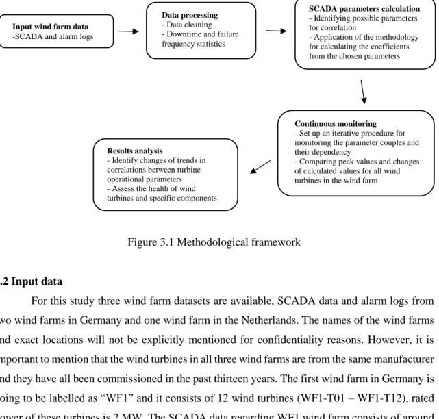
This project focuses on an application for processing wind farm operational data and extracting valuable information that can be useful to wind farm operators. Therefore, a methodological framework for this approach has been developed, see Figure 3.1. The methodology requires SCADA and alarm logs as input information, and consists of the following steps: 1) data processing, 2) SCADA parameters calculation, 3) continuous monitoring, 4) Results analysis. Each of the steps in the framework will be explained further in this chapter.
Figure 3.1 Methodological framework
3.2 Input data
For this study three wind farm datasets are available, SCADA data and alarm logs from two wind farms in Germany and one wind farm in the Netherlands. The names of the wind farms and exact locations will not be explicitly mentioned for confidentiality reasons. However, it is important to mention that the wind turbines in all three wind farms are from the same manufacturer and they have all been commissioned in the past thirteen years. The first wind farm in Germany is going to be labelled as “WF1” and it consists of 12 wind turbines (WF1-T01 – WF1-T12), rated power of these turbines is 2 MW. The SCADA data regarding WF1 wind farm consists of around
Input wind farm data -SCADA and alarm logs
Data processing - Data cleaning - Downtime and failure frequency statistics
Continuous monitoring - Set up an iterative procedure for monitoring the parameter couples and their dependency
- Comparing peak values and changes of calculated values for all wind turbines in the wind farm Results analysis
- Identify changes of trends in correlations between turbine operational parameters - Assess the health of wind turbines and specific components
SCADA parameters calculation - Identifying possible parameters for correlation
- Application of the methodology for calculating the coefficients from the chosen parameters
32 months of data, from the period of installation until the 3rd year of operation. The second wind
farm in Germany is going to be labelled as “WF2” and it has 14 wind turbines (T01 – WF2-T14) with 2 MW rated power. The amount of SCADA data available is close to 67 months, between the 5th and 10th year of wind farm operation. Finally, the wind farm in the Netherlands is
going to be labelled as “WF3” and it contains 28 wind turbines (WF3-T01 – WF3-T28) each with 850 kW rated power. The available data regarding WF3 wind farm consists of around 25 months of SCADA data in the period between the 8th and 10th year of wind farm operation.
3.3 Data processing
All of the data processing in this project was done in Microsoft Excel and Matlab, however the data was originally stored in Microsoft SQL Server database. Both the SCADA and the alarm logs have to be pre-processed before they can be used in the application. The alarm data is logged in code numbers, or designated sentences, which can be interpreted with user manuals for specific wind turbines. However, even with the user manual the origin of the fault isn’t always evident and sometimes cannot be assigned to a specific subassembly. Also, as it was mentioned before, the available SCADA data is usually not complete and contains only a fraction of the parameters that are recommended by the IEC standard. Additionally, SCADA logs have to be checked for false entries which are to be removed. These difficulties are to be expected when working with data gathered from operating wind farms.
3.3.1 Wind turbine taxonomy
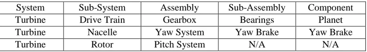
Available data from three different wind farms is going to be used for this project, all of the wind turbines in these wind farms are three bladed, pitch controlled and contain a gearbox. When analysing the alarm logs of a wind farm it is important to differentiate turbine components that are reported as origin of a failure. During the analysis of alarm logs a universal taxonomy of wind turbines has been used. This taxonomy, developed by Tavner (2011), has been applied in the ReliaWind project. The proposed taxonomy separates a wind turbine into 5 levels which are system, sub-system, assembly, sub-assembly and component. An example of the taxonomy is given in Table 3.1.
Table 3.1 Example of the taxonomy used in ReliaWind, Source: Tavner, 2011
System Sub-System Assembly Sub-Assembly Component
Turbine Drive Train Gearbox Bearings Planet
Bearings
Turbine Nacelle Yaw System Yaw Brake Yaw Brake
Disc
Turbine Rotor Pitch System N/A N/A
However, the alarm logs usually do not contain enough information to define the exact location of the fault that was detected. Thus, the analysis in this paper will be based on the sub-system and assembly level. For more detailed investigation, additional data sources like maintenance logs and purchase bills are needed.
3.3.2 Availability calculation
In the IEC standard available information regarding the operational state of a wind turbine is divided in informational categories. Most importantly there are two informational categories that represent the first mandatory level of information. Those two categories are (The International Electrotechnical Commission, 2011):
Information available (IA) Information unavailable (IU)
The IA category branches out into subcategories which are:
Information available operative category (IAO) Information available non operative category (IAN) Information available force majeure category (IAFM)
Under the IAO category there are two subcategories that are important for the availability calculation, those are:
Information available operative generating category (IAOG) Information available operative non generating category (IAONG)
Also, one optional subcategory under the IAONG has to be defined for the calculation of system operational availability, that subcategory is:
Information available operative non generating out of environmental specification optional category - calm winds (IAONGENC)
With this optional subcategory a distinction is made between non-operating hours due to low wind resources and due to other operating conditions. This way in case of low winds the turbine is considered as available. However, it is important to notice that this calculation does not differentiate the downtime caused by grid failure from the downtime of the turbine. For the sake of brevity all other availability subcategories will not be defined in this paper as they are not essential for understanding operational availability. Now when the necessary categories and subcategories are defined it is easy to calculate operational availability that is going to be used for the data analysis. For the availability of wind turbines the following formula is applied:
Availability = 1 - Unavailability = 1 - Unavailable time
Available time + Unavailable time (3.1)
In the equation (3.1) the summation of the time categories IAOG and IAONGENC represent the “Available time”, summation of all other categories is the “Unavailable time”. The exception is the IU category which is not considered in this calculation. Therefore, in written form the system operational availability is:
Availability = 1 - IAOG+IAONGENC+(IAONG-IAONGENC)+IAN+IAFM(IAONG-IAONGENC)+IAN+IAFM (3.2)
This way it is easy to calculate the availability of each turbine in a wind farm in the same way, which will be applied on data from all three wind farms.
3.3.3 MTBF, MTTF & MTTR
The reliability metrics will also be presented for all of the turbines, the purpose of this is to show the range of values for MTBF, MTTF and MTTR in different wind farms. It is important to emphasize the fact that the reliability metrics are going to be calculated directly from the alarm
logs. In the alarm logs every alarm instance is considered equal, without regards to the magnitude of the failure or the amount of downtime. This means that the MTBF is going to be calculated as an average time between alarms and these alarms are not necessarily critical faults. Also, the values that will be presented as reliability metrics are calculated for each wind turbine and not for separate turbine components. The value for MTBF will be calculated by dividing the time covered by the alarm logs with the number of alarm instances reported in that period. The MTTR can be calculated as an average downtime for a turbine, it represents the mean length of an alarm. Subsequently, the value for MTTF is easy to calculate as the difference between the MTBF and MTTR for the same wind turbine.
3.4 SCADA data monitoring application
A methodology for extracting valuable information from SCADA logs is going to be structurally presented and explained in this chapter. Initially, raw SCADA data is collected as 10-minute averages which need to be pre-processed before they can be used in the monitoring application. The processing approach is based on a methodology presented by Yang et al. (2013). First step for preparing the SCADA data for correlation is to define the parameters of interest, which is relying on available data. There are several SCADA parameters that are recorded in all of the three wind farms whose data is available for analysis. Those parameters are:
Local ID Time stamp Wind speed Rotor speed Generator speed Generator power Turbine OK counter Environment temperature Generator temperature Gearbox temperature
Fortunately, the parameters listed above are among the most commonly monitored SCADA parameters. Observing the relation between two parameters of choice can help explaining the idea
behind the proposed methodology. If two parameters are correlated as 10-minute values, without any processing, the dependency is not easy to detect. Therefore, binning of the parameters is done to merge the raw SCADA data and present it as a sorted correlation of parameters. Wind speed will be used as a reference parameter for binning the parameter of interest in the following example. Prior to the binning process the SCADA data has to be filtered in order to delete the data that was collected while the wind turbine was not generating power. At this point all of the SCADA lines in which the power parameter is equal to zero should be deleted. Additionally, the information from the “Turbine OK counter” column can be useful for identifying instances when the turbine was unavailable. Afterwards, the wind speed and the selected parameter for binning need to be categorised by the following algorithm developed by Yang et al. (2013).
For the purpose of binning, the maximum and minimum wind speed, 𝑉𝑚𝑖𝑛 and 𝑉𝑚𝑎𝑥 should be identified from the SCADA logs wind speed column. After that the binning step can be set, for example 𝑉𝑠𝑡𝑒𝑝= 0.5, and the range of wind speeds from 𝑉𝑚𝑖𝑛 to 𝑉𝑚𝑎𝑥 can be divided in 𝑁 number of bins, where
𝑁 =𝑉𝑚𝑎𝑥−𝑉𝑚𝑖𝑛
𝑉𝑠𝑡𝑒𝑝 . (3.3)
The iteration process starts by defining the range [𝑉𝑚𝑖𝑛+ (𝐾 − 1) × 𝑉𝑠𝑡𝑒𝑝, 𝑉𝑚𝑖𝑛+ 𝐾 × 𝑉𝑠𝑡𝑒𝑝] in which the located wind speed indices 𝐼 are recorded, where 𝐾 = 1 for the first iteration. The statistical analysis of wind speed data in the 𝐾-th subrange is done by dividing the subrange further into 𝑚 bins and then calculating the expected value of the wind speed as
𝑉̅𝐾= ∑𝑚𝑗=1(𝑝𝑗× 𝑣𝑗) 𝑗 =(1,2, … 𝑚) (3.4)
Where 𝑝𝑗= 𝑛𝑗⁄ × 100% is the frequency function giving the probability that the wind speed is 𝑛 located in the 𝑗-th bin, 𝑛𝑗 is the number of wind speed indices in the 𝑗-th bin and 𝑛 is the total number of wind speed data in the 𝐾-th subrange; 𝑣𝑗 represents to corresponding wind speed in the 𝑗-th bin. For the purpose of this analysis the number of bins 𝑚 is equal to 5 bins. The same method is used to analyse other valuable SCADA parameters, for example generator power data can be binned with the following formula
𝑃̅𝐾= ∑𝑚 (𝑝′𝑗× 𝑃𝑗) 𝑗 =
𝑗=1 (1,2, … 𝑚) (3.5)
where [𝑝′
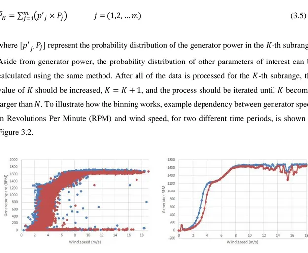
𝑗, 𝑃𝑗] represent the probability distribution of the generator power in the 𝐾-th subrange. Aside from generator power, the probability distribution of other parameters of interest can be calculated using the same method. After all of the data is processed for the 𝐾-th subrange, the value of 𝐾 should be increased, 𝐾 = 𝐾 + 1, and the process should be iterated until 𝐾 becomes larger than 𝑁. To illustrate how the binning works, example dependency between generator speed in Revolutions Per Minute (RPM) and wind speed, for two different time periods, is shown in Figure 3.2.
a) b)
Figure 3.2 Example generator speed and wind speed correlation extracted from SCADA data; blue and red dots and lines represent two different time periods
a) plot of 10-minute values b) 10-minute values after binning
The 10-minute average values gathered from the raw SCADA data are shown in Figure 3.2 a. These values can be approximated by curves calculated with the binning algorithm, which can be seen in Figure 3.2 b. The two curves from the Figure 3.2 b represent the dependency of the generator speed and wind speed for two different time periods. The idea behind the proposed methodology is to quantify the deterioration of a certain component by comparing the correlation of relevant SCADA parameters and their change over time. Respectively, the methodology for condition monitoring through SCADA data is actually calculating the change of the dependency over a period of time, the approach for this will be described in the following subchapter.
3.4.1 Calculating the coefficient representing the state of the component
The reasoning behind the methodology developed by Yang et al. (2013) was shown in the previous subsection, and now the approach that was used for comparing relevant parameter correlations is going to be presented. First of all, the correlation between two parameters {𝑥𝑖, 𝑦𝑖}(𝑖 = 1,2, … , 𝑛) can be represented by the following equation
𝑦̂𝑖 = 𝑎0+ 𝑎1𝑥𝑖+ 𝑎2𝑥𝑖2+ ⋯ + 𝑎
𝑘𝑥𝑖𝑘 (3.6)
where 𝑎𝑗 (𝑗 = 1,2, … , 𝑘) represents the model coefficients, 𝑘 is the order of the equation (𝑘 = 4 in all of the calculations) and 𝑦̂𝑖 is the estimation of the parameter 𝑦𝑖. This equation can be written in matrix form, as shown in the following equation
𝒀 = 𝑿 ∗ 𝑨. (3.7)
With this approach the parameter 𝑦𝑖, shown as matrix Y, is being estimated with the parameter 𝑥𝑖 and coefficients 𝑎𝑗, matrices 𝑿 and 𝑨, respectively. The best estimation of 𝑦𝑖 can be achieved if the following conditions are satisfied in accordance with the least squares principles, i.e.
{ 𝜕(𝑅2) 𝜕𝑎0=0 𝜕(𝑅2) 𝜕𝑎1=0 ⋮ 𝜕(𝑅2) 𝜕𝑎𝑘=0 (3.8)
where the total estimation error is referred to as 𝑅2= ∑ |𝑦
𝑖− 𝑦̂𝑖|2 𝑛
𝑖=1 . If the value for 𝑦̂𝑖 from (3.6) is substituted into (3.8) the resulting equation is a Vandermonde matrix equation
[ 𝑛 ∑𝑛𝑖=1𝑥𝑖 ⋯ ∑𝑛𝑖=1𝑥𝑖𝑘 ∑𝑛 𝑥𝑖 𝑖=1 ∑𝑛𝑖=1𝑥𝑖2 ⋯ ∑𝑛𝑖=1𝑥𝑖𝑘+1 ⋮ ⋮ ⋱ ⋮ ∑𝑛 𝑥𝑖𝑘 𝑖=1 ∑𝑛𝑖=1𝑥𝑖 ⋯ ∑𝑛𝑖=1𝑥𝑖2𝑘 ] [ 𝑎0 𝑎1 ⋮ 𝑎𝑘 ] = [ ∑𝑛 𝑦𝑖 𝑖=1 ∑𝑛 𝑥𝑖𝑦𝑖 𝑖=1 ⋮ ∑ 𝑥𝑖𝑘𝑦 𝑖 𝑛 𝑖=1 ] (3.9)
[ 1 𝑥1 ⋯ 𝑥1𝑘 1 𝑥2 ⋯ 𝑥2𝑘 ⋮ ⋮ ⋱ ⋮ 1 𝑥𝑛 ⋯ 𝑥𝑛𝑘] [ 𝑎0 𝑎1 ⋮ 𝑎𝑘 ] = [ 𝑦1 𝑦2 ⋮ 𝑦𝑛 ] (3.10)
Afterwards, if both sides of the (3.10) equation are multiplied with the transpose of the first matrix the new equation is
[ 1 1 ⋯ 1 𝑥1 𝑥2 ⋯ 𝑥𝑛 ⋮ ⋮ ⋱ ⋮ 𝑥1𝑘 𝑥 2𝑘 ⋯ 𝑥𝑛𝑘 ] [ 1 𝑥1 ⋯ 𝑥1𝑘 1 𝑥2 ⋯ 𝑥2𝑘 ⋮ ⋮ ⋱ ⋮ 1 𝑥𝑛 ⋯ 𝑥𝑛𝑘] [ 𝑎0 𝑎1 ⋮ 𝑎𝑘 ] = [ 1 1 ⋯ 1 𝑥1 𝑥2 ⋯ 𝑥𝑛 ⋮ ⋮ ⋱ ⋮ 𝑥1𝑘 𝑥 2𝑘 ⋯ 𝑥𝑛𝑘 ] [ 𝑦1 𝑦2 ⋮ 𝑦𝑛 ] (3.11)
and now the following matrices can be defined
𝑿 = [ 1 𝑥1 ⋯ 𝑥1𝑘 1 𝑥2 ⋯ 𝑥2𝑘 ⋮ 1 ⋮ 𝑥𝑛 ⋱ ⋮ ⋯ 𝑥𝑛𝑘] , 𝑨 = [ 𝑎0 𝑎1 ⋮ 𝑎𝑘 ] , 𝒀 = [ 𝑦1 𝑦2 ⋮ 𝑦𝑛 ] . (3.12)
This way equation (3.11) can be written as
𝑿𝑇𝑿𝑨 = 𝑿𝑇𝒀. (3.13)
Ultimately, the estimation of 𝑎𝑗 coefficients can be calculated by solving the following matrix equation
𝑨 = (𝑿𝑇𝑿)−1𝑿𝑇𝒀, (3.14)
Furthermore, matrix 𝑨 and coefficients 𝑎𝑗 represent the dependency of two chosen parameters during a fixed time interval from which the data was collected. To assess the current state of a turbine part the methodology extends to comparing the value of the matrix 𝑨 calculated from present data with a new matrix calculated from the historic data. Matrix 𝑩 and its coefficients 𝑏𝑗 are introduced for this purpose as they represent the model dependence derived from the historic
data. Finally, formula for calculating the coefficient 𝑐 that is used for assessing the condition of specific turbine parts is
𝑐 =∫ |∑ (𝑎𝑗−𝑏𝑗)𝑥 𝑗 𝑘 𝑗=0 |𝑑𝑥 𝑥𝑚𝑎𝑥 𝑥𝑚𝑖𝑛 𝑥𝑚𝑎𝑥−𝑥𝑚𝑖𝑛 . (3.15)
In the equation (3.15) 𝑥𝑚𝑎𝑥 and 𝑥𝑚𝑖𝑛 are the maximum and minimum values of parameter 𝑥𝑖 from the present data, respectively. The value of the coefficient 𝑐 represents the health assessment of a certain part. If the coefficient is 𝑐 ≈ 0 than the part is considered healthy, as the 𝑨 and 𝑩 matrices values have similar values. If the coefficient value is 𝑐 > 0 the condition of the part is deteriorating or there has been a fault occurrence. Furthermore, with the turbine part of interest being in more severe state the value of the 𝑐 coefficient tends to be larger. Additionally, in relation to the Figure 3.2 b the coefficients 𝑎𝑗 and 𝑏𝑗 describe the properties of the two curves that represent the dependency between two parameters from different time periods. Therefore, if the example from Figure 3.2 b was to be analysed, the 𝑐 coefficient would be a numerical value that represents the difference between two lines. A model was developed in Matlab to calculate the needed matrices and equations. This model compares two different parameters from SCADA data and determines their dependence. By monitoring these parameters and how their dependence changes with time, a substantial amount of information regarding the condition of a specific turbine part can be acquired.
3.5 Continuous monitoring
Now that the calculation of the 𝑐 coefficient is explained, there are several difficulties that need to be resolved in order to adequately monitor specific wind turbine components. The methodology that was previously described does not define some of crucial application details. Therefore, the goal of this paper is to create the most appropriate application for monitoring health of wind turbine components. During the development of the Matlab model several potential issues were noticed and had to be taken into consideration in order to have a successful application of the methodology. The main observations regarding these issues were:
- As it was mentioned in the original paper, the distribution and range of the data used for comparison affects the accuracy of the model. Since the methodology is based on
comparing two datasets, the range in which this data is presented can lead to uneven representation of the turbine state. Also, the density of data in certain range can be influenced by higher or lower than average values of parameters in the observed period, this also can affect the accuracy of the model.
- In order to compare the component state of wind turbines in a wind farm, the amount of data used for representation of each period should be the same, or at least similar, for all turbines. The number of SCADA lines, or number of data points, used for describing the present or historical data affects the results of the application.
- The ratio of the parameters that are to be used for the comparison affects the value of the 𝑐 coefficient. This effect can lead to results that have higher values than expected and that can be misinterpreted as critical. However, for the application at hand and comparing turbines and their components in a wind farm, this effect can be disregarded as it is the same for all turbines in a wind farm. Normalisation of the parameters can solve this problem if needed.
These observations about the application of the model indicate certain constraints that have to be considered during the calculations. With these limitations in mind the application was developed in such a way to assure the best possible accuracy. First of all, the datasets from the three wind farms that are available for application is in range from around two to five years of SCADA data. Ideally, the historic data would be available from the period of time that can be considered as normal operation, the data from early years of operation would be most valuable. However, because the early historical data is not always available, the monitoring approach was developed with systematically increasing amount of historical data through iterations. The available SCADA datasets are to be divided in equal partitions and then an iterative approach can be applied. The matrix 𝑨 that represents present data in each iteration is to be calculated from the data contained in every partition separately. This means that every partition will be represented by a separate matrix 𝑨, meanwhile the matrix 𝑩 that represents the historical data is to be calculated with an increasing amount of data with every iteration. In comparison with the matrix 𝑨, the matrix 𝑩 is to be calculated with all of the preceding available data in each iteration. This way the coefficient 𝑐 can be calculated for each partition of the SCADA data which allows continuous monitoring of turbine components.
During the first testing phase another problem had to be addressed, as it was mentioned before the amount of SCADA data in each partition impacts the accuracy of the model. In order to unify the amount of data, in this case the number of SCADA lines, in each partition additional data filtering had to be performed. In collaboration with the Project Engineer from Mecal the decision was made to use only the SCADA lines with the time stamps that are present in all of the wind turbines data in a wind farm (Links, 2016). Illustration of the additional filtering process of SCADA data on an exemplary wind farm containing three turbines is shown in Table 3.2
Table 3.2 Illustration showing the additional filtering process. Only the data from the periods when data is available for all of the turbines in the analysis is to be used in the calculations,
Source: Links, 2016
Period 1 Period 2 Period 3 Period 4 Period 5 WTG1 Available Available Available Unavailable Unavailable WTG2 Unavailable Available Available Available Unavailable WTG3 Unavailable Unavailable Available Available Available Filtered Unavailable Unavailable Available Unavailable Unavailable
Essentially, the additional filtering leaves only the available data created when all of the turbines in a wind farm were operating at the same time. Unfortunately, this action severely reduces the amount of data for comparison. The amount of available data for all wind farms, in per cents of original SCADA data, after each filtering process is shown in Table 3.3.
Table 3.3 Statistics of available SCADA data after the filtering processes
Wind farm Number of turbines
Available data after filtering false entries and standby data [%]
Available data after additional filtering [%]
WF1 12 78 48
WF2 14 68 26
WF3 28 70 10
With more wind turbines in a wind farm the additional filtering process reduces a greater amount of SCADA data, which can be seen in Table 3.3. However, this kind of filtering creates equal partitions of SCADA data for comparison. Because of that all of the starting and ending points of partitions are known and equal for all wind turbines in a wind farm, which is convenient for
continuous comparison of the turbine components and coefficient values. Unfortunately, the amount of SCADA lines is equal in each partition but the time length of each partition can vary.
3.5.1 Testing methodology and potential correlations
After the pre-processing of the available SCADA data and the chosen parameters for monitoring, the next step is to investigate the potential correlations. The parameters that are available for this project are most suitable for the condition monitoring of the gearbox and the generator. With more data the methodology could be applied to assess the state of other wind turbine parts. However, gearbox and generator are critical wind turbine components and, as it was mentioned before, failures of the gearboxes result in the longest downtime compared to any other turbine part. Potential correlations that are available for investigation are (Yang, et al., 2013):
1. Rotor speed (RPM) / Generator power
- correlation between these parameters is used for monitoring gearbox health 2. Rotor speed (RPM) / Generator speed (RPM)
- also used for monitoring gearbox health 3. Rotor speed (RPM) / Gearbox temperature
- miscorrelation between these two parameters indicates a fault occurrence in gearbox 4. Generator speed (RPM) / Generator power
- used for monitoring of generator health
Upon further analysis it has been shown that dependency between rotor speed and generator speed cannot be taken into consideration. Monitoring the correlation of rotor and generator speed with a high sampling frequency can be useful for detecting the subtle changes of the state of gears in the gearbox. However, this application is not valuable if done with 10-minute values because the information about the health of gears is lost with the averaging of values. Furthermore, because of the same reason, monitoring of the rotor speed and the generator power shows reciprocal results to monitoring of the generator speed and power, which is used for monitoring generator health. Therefore, these two couples of SCADA parameters have to be excluded in this analysis.
3.6 Results analysis
After the application the acquired results should be interpreted and analysed to determine the value of the gathered information and further steps. One of the goals of this project is to develop a tool for SCADA data processing and extracting information that can be valuable to wind farm owners, operators and consulting companies. Ideally, the use of the correlation technique could highlight critical wind turbines and wind turbine components and give an insight regarding their deterioration and health. With this kind of information wind farm operators can make more informed decisions in regard to maintenance planning and inspections scheduling. Also, consulting companies could potentially use this application as an additional tool for maintenance optimization or life extension prediction. After the application of the methodology and results chapter, in the discussion and conclusion chapters, these properties of the application will be analysed together with other potential functions for the proposed methodology.
CHAPTER 4. APPLICATION OF THE METHODOLOGY AND RESULTS
4.1 Introduction
Downtime statistics for the three wind farms have been extracted from the available alarm logs. The downtime will be categorised in accordance with the turbine taxonomy presented in previous chapter. Furthermore, to describe the wind farms more accurately, the availability, MTBF, MTTR, MTTF values together with average values of wind speed, generator temperature and gearbox temperature will be shown for each wind turbine. All of these values and the downtime statistics are used to describe the wind farms more accurately, with that information the wind farms can be compared and verified as regular in accordance with the published statistics. Afterwards, the SCADA data monitoring can be applied and example applications will be presented for each wind farm.
4.2 Downtime statistics
Downtime statistics of the WF1 wind farm can be seen in Figure 4.1.
From Figure 4.1 it is obvious that failures caused by the control system and nacelle hydraulic system cause the most downtime. When it comes to frequency of failures, alarms are most often caused by malfunctions of the yaw system, generator and the converter. Additional information regarding availability, reliability and average values of relevant SCADA parameters is shown in Table 4.1.
Table 4.1 Availability, reliability and average values of parameters for the WF1 wind farm
WF1 Availa-bility [%] MTBF [h] MTTR [h] MTTF [h] Average wind speed [m/s] Average generator temp. [°C] Average gearbox temp. [°C] T01 99,18 69:11:56 0:33:58 68:37:57 5,81 64,17 50,26 T02 99,45 78:29:14 0:26:07 78:03:07 6,09 56,42 50,56 T03 98,37 69:36:39 1:08:14 68:28:24 5,40 53,51 47,05 T04 99,34 98:41:19 0:39:14 98:02:05 5,69 56,32 47,61 T05 99,56 146:10:57 0:38:32 145:32:25 5,46 54,02 51,20 T06 99,52 97:03:02 0:28:04 96:34:58 5,68 62,22 49,44 T07 98,82 109:48:30 1:17:54 108:30:36 5,71 53,60 48,16 T08 98,20 102:08:10 1:50:33 100:17:38 5,86 55,11 48,07 T09 99,37 80:22:31 0:30:20 79:52:11 5,47 71,65 48,81 T10 99,18 78:45:05 0:38:45 78:06:21 5,15 58,98 48,18 T11 99,58 99:06:24 0:24:53 98:41:32 5,47 61,40 48,61 T12 98,97 92:05:00 0:57:04 91:07:56 5,73 55,16 49,06
The statistics from Table 4.1 show that all of the turbines in WF1 wind farm have availability in the range from 98,2 to 99,97 %, which can be considered very high. The MTBF and MTTR values show that for the turbines in the WF1 wind farm alarms occur on average once in 93 hours and are resolved within 48 minutes. The results shown in Figure 4.1 and Table 4.1 are the first steps of wind farm analysis, this information will be used for comparison with other wind farms.
The downtime statistics of the WF2 wind farm are shown in Figure 4.2, while additional statistics can be seen in Table 4.2.
Figure 4.2 Failure occurrences and downtime statistics for the WF2 wind farm
Table 4.2 Availability, reliability and average values of parameters for the WF2 wind farm
WF2 Availa-bility [%] MTBF [h] MTTR [h] MTTF [h] Average wind speed [m/s] Average generator temp. [°C] Average gearbox temp. [°C] T01 97,44 164:25:55 4:12:12 160:13:43 5,41 48,25 45,02 T02 97,27 97:25:45 2:39:43 94:46:01 5,05 48,95 47,66 T03 96,83 96:06:17 3:02:38 93:03:39 5,35 60,67 44,54 T04 97,52 108:03:56 2:40:46 105:23:10 4,89 65,25 48,23 T05 99,13 749:54:33 6:30:45 743:23:47 5,27 62,94 47,25 T06 95,41 135:36:00 6:13:35 129:22:25 5,73 69,74 49,78 T07 98,03 121:36:25 2:23:59 119:12:26 5,21 62,69 49,30 T08 97,84 122:48:50 2:39:21 120:09:29 5,35 61,41 48,38 T09 96,24 117:17:04 4:24:27 112:52:36 4,86 45,43 49,18 T10 96,09 113:46:46 4:26:50 109:19:56 4,88 62,19 46,37 T11 96,42 97:02:49 3:28:15 93:34:34 5,31 58,25 46,58 T12 96,60 119:33:03 4:03:49 115:29:14 5,46 62,73 49,91 T13 97,21 72:40:42 2:01:45 70:38:57 5,42 62,46 51,98 T14 96,59 77:05:36 2:37:42 74:27:55 5,29 58,69 48,95
The statistics from Figure 4.2 show that the highest downtime in WF2 wind farm is caused by faults occurring in the control system, grid connection and nacelle hydraulic system. The highest alarm frequency is caused by the converter, generator, control system and the gearbox, respectively. Results from Table 4.2 show that the availability of the WF2 wind farm is lower than the availability of WF1 wind farm, which is to be expected as WF2 wind farm is older. However, reliability metrics show that alarms where less frequent but the average time to repair was significantly higher in the WF2 wind farm, compared to the WF1 wind farm.
Finally, the downtime statistics of the WF3 wind farm can be seen in Figure 4.3.
Figure 4.3 Failure occurrences and downtime statistics for the WF3 wind farm
Figure 4.3 presents the statistics for WF3 wind farm and shows that the failures caused by the control system, gearbox and the grid connection cause the most downtime. However, the highest number of alarm occurrences originates from the electrical converter, gearbox and generator. Availability statistics and other important statistics are shown in Table 4.3.
Table 4.3 Availability, reliability and average values of parameters for the WF3 wind farm WF3 Availa-bility [%] MTBF [h] MTTR [h] MTTF [h] Average wind speed [m/s] Average generator temp. [°C] Average gearbox temp. [°C] T01 96,94 40:25:11 1:14:17 39:10:54 5,37 53,45 50,52 T02 98,19 63:05:39 1:08:39 61:57:00 6,35 54,65 57,79 T03 98,44 113:31:48 1:46:33 111:45:15 5,63 54,17 53,00 T04 96,78 54:12:56 1:44:48 52:28:08 5,90 53,01 51,30 T05 99,25 179:17:14 1:20:32 177:56:42 6,04 60,97 52,42 T06 97,09 63:25:32 1:50:50 61:34:42 5,02 46,88 54,97 T07 96,91 50:26:25 1:33:27 48:52:58 4,43 46,08 51,17 T08 98,25 60:15:35 1:03:15 59:12:20 5,78 57,92 53,38 T09 94,57 35:53:35 1:56:50 33:56:45 6,08 26,17 50,60 T10 99,23 210:33:30 1:37:30 208:55:59 5,34 66,30 56,66 T11 96,90 33:45:08 1:02:46 32:42:21 5,37 59,89 51,02 T12 97,84 97:05:38 2:05:56 94:59:42 5,62 57,27 54,83 T13 98,97 123:11:02 1:15:55 121:55:06 5,36 51,57 57,21 T14 98,27 97:37:02 1:41:32 95:55:31 4,81 54,87 54,00 T15 99,10 127:04:26 1:08:41 125:55:44 5,81 60,58 52,25 T16 96,59 44:55:59 1:31:49 43:24:10 5,56 56,17 49,64 T17 98,15 76:24:18 1:24:55 74:59:24 5,67 56,59 52,82 T18 98,07 56:03:43 1:05:04 54:58:39 5,87 54,29 49,32 T19 97,70 97:21:18 2:14:23 95:06:55 5,97 57,01 55,38 T20 97,69 45:33:17 1:03:07 44:30:10 5,71 57,34 51,19 T21 94,68 51:17:51 2:43:51 48:34:00 5,46 57,86 53,51 T22 97,27 30:36:49 0:50:13 29:46:36 4,20 46,45 50,21 T23 98,35 38:56:31 0:38:32 38:17:59 5,35 52,64 55,27 T24 94,58 60:39:48 3:17:08 57:22:40 4,28 42,50 55,34 T25 98,95 117:58:03 1:14:37 116:43:26 4,55 50,85 53,41 T26 96,61 34:31:28 1:10:07 33:21:20 4,80 47,24 51,36 T27 95,88 36:39:21 1:30:32 35:08:49 4,14 46,91 53,99 T28 96,61 24:50:22 0:50:30 23:59:52 4,50 46,51 49,38
Statistics from Table 4.3 show the high level of diversity among the reliability of wind turbines in the WF3 wind farm. The availability of wind turbines varies from below 95 % to over 99 % and the frequency of alarm occurrences, as well as the average time to repair, is also significantly differing for each turbine.
The statistics from the three wind farms presented above show the diversity of downtime sources in different wind farms and the varying frequency of alarms among different turbine
components. It can be concluded that the control system causes the highest downtime in all three wind farms, followed by the gearbox, grid connection, nacelle hydraulic system and the generator. Unfortunately, components like the control system and nacelle hydraulic system cannot be adequately monitored with the proposed SCADA monitoring application. Also, the downtime originating from the grid connection is often not related to the turbine health as it is usually caused by curtailment or power grid congestion. Therefore, the analysis will proceed with the generator and gearbox monitoring through SCADA data.
4.3 Generator monitoring
The first application examples are going to be performed with the SCADA data from the WF1 wind farm, explicitly monitoring the generator through the generator speed (RPM) and power production. The WF1 wind farm was chosen for generator monitoring because it was previously known that there have been changes in control software of the wind turbines. Specifically, during the period of time with available SCADA data the power curves of the wind turbines in the WF1 wind farm have been altered in order to maximize annual production. For the application, this adjustment of the power curve is not a reason for generator deterioration; however, the power curve modification should be recognised by the SCADA monitoring methodology. Also, it is important to mention that in the WF1 wind farm statistics the generator is not among the main downtime sources and the available SCADA data is from the first three years of wind farm operation. Therefore, the power curve change detection should be easier to detect, as no notable generator deterioration or failures are to be expected. If there was a control software update and the power curve was modified, the dependence of the generator speed and power production must have been affected, too. The results of this comparison will be used for verification of the monitoring application, and for investigating the full potential of the methodology and application.
The first example was performed without applying the additional filtering process that was described in the previous chapter and illustrated in Table 3.2. This was done in order to assess the impact of additional data filtering on the model and its accuracy. Therefore, in the first example the available data for each turbine was divided in 20 partitions and the number of individual SCADA lines in each partition was different for each wind turbine, varying from 5000 to 5800 SCADA lines per partition. The historical data was increased with every iteration, as it was explained in the previous chapter, and each one of the SCADA data partitions were used as present data for comparison with historical data. The iterative calculation produced 20 consecutive values

![Table 2.2 Reliability of generators, gearboxes and converters, Source: Spinato et al., 2008 Subassembly Failure rate [failure/year] MTBF [h]](https://thumb-eu.123doks.com/thumbv2/5dokorg/5508603.143524/18.918.153.797.883.974/reliability-generators-gearboxes-converters-source-spinato-subassembly-failure.webp)