Differences of Type I error rates for ANOVA and Multilevel-Linear-Models using SAS and SPSS for repeated measures designs

Published under the CC-BY4.0 license

Open reviews and editorial process: Yes

Preregistration: No All supplementary files can be accessed at the OSF project page: https://osf.io/em62j/

Differences of Type I error rates for ANOVA and

Multilevel-Linear-Models using SAS and SPSS for repeated measures

designs

Nicolas Haverkamp

University of Bonn

André Beauducel

University of Bonn

To derive recommendations on how to analyze longitudinal data, we examined Type I error rates of Multilevel Linear Models (MLM) and repeated measures Analysis of Variance (rANOVA) using SAS and SPSS. We performed a simulation with the following specifications: To explore the effects of high numbers of measurement occasions and small sample sizes on Type I error, measurement occasions of m = 9 and 12 were investigated as well as sample sizes of n = 15, 20, 25 and 30. Effects of non-sphericity in the population on Type I error were also inspected: 5,000 random samples were drawn from two populations containing neither a within-subject nor a between-group effect. They were analyzed including the most common options to correct rANOVA and MLM-results: The Huynh-Feldt-correction for rANOVA (rANOVA-HF) and the Kenward-Roger-correction for MLM (MLM-KR), which could help to correct progressive bias of MLM with an unstructured covariance matrix (MLM-UN). Moreover, uncorrected rANOVA and MLM assuming a compound symmetry covariance structure (MLM-CS) were also taken into account. The results showed a progressive bias for MLM-UN for small samples which was stronger in SPSS than in SAS. Moreover, an appropriate bias correction for Type I error via rANOVA-HF and an insufficient correction by MLM-UN-KR for n < 30 were found. These findings suggest MLM-CS or rANOVA if sphericity holds and a correction of a violation via rANOVA-HF. If an analysis requires MLM, SPSS yields more accurate Type I error rates for CS and SAS yields more accurate Type I error rates for MLM-UN.

Keywords: Multilevel linear models, software differences, repeated measures ANOVA,

simulation study, Kenward-Roger correction, Type I error rate

In times of a replication crisis that is yet to over-come, we feel a need to improve methodological standards in order to regain credibility of scientific knowledge. It is therefore important to generate clearly formulated “best practice” recommendations when there are multiple competing methodological approaches for the same issue in question. Progress in psychology means for researchers to understand

and investigate their methodological tools in order to know about their strengths and weaknesses as well as the circumstances under which they should or should not be used.

In this study, we will therefore focus on two pop-ular methods to analyze dependent means as they occur, for example, in longitudinal data. It is im-portant to examine whether a mean change over time is of statistical relevance or not. In recent lon-gitudinal research, a trend to use Multilevel linear

Correspondence Address: Dr. Nicolas Haverkamp, Institute of Psychology, University of Bonn, Kaiser-Karl-Ring 9, 53111 Bonn, Germany. nicolas.haverkamp@uni-bonn.de

HAVERKAMP & BEAUDUCEL

2

models (MLM) instead of repeated measures analy-sis of variance (rANOVA) can be identified (Arnau, Balluerka, Bono, & Gorostiaga, 2010; Arnau, Bono, & Vallejo, 2009; Goedert, Boston, & Barrett, 2013; Gueorguieva & Krystal, 2004); even appeals to re-searchers in favor of MLM over rANOVA are made (Boisgontier & Cheval, 2016). Despite the high popu-larity of MLM, the terminology is not all clear with-out ambiguity. We follow a definition of Tabachnick and Fidell (2013) in using the term “MLM” to denote models with the following characteristics: Regres-sion models basing upon at least two data levels, where the levels are typically specified by the meas-urement occasions interleaved with individuals, models containing covariance pattern models, and fixed as well as random effects. Although Tabach-nick and Fidell (2013, p. 788) indicate that “MLM” is used for “a highly complex set of techniques”, they mention the presence of at least two data levels first, giving the impression that this is the most important aspect of these techniques. As we noticed massive differences in Type I error rates for different ap-proaches before (Haverkamp & Beauducel, 2017), we will furthermore focus on the Type I error correc-tions that are offered by the respective method. Moreover, the large Type I errors that we have no-ticed before could trigger publications of results that cannot be replicated or reproduced. This is why we consider that the focus on Type I error rates is of special importance for the current debate on the re-producibility of results.

If the features of MLM over rANOVA are com-pared, three main advantages of MLM become ap-parent: First, MLMs permit to model data that are structured in at least one level. If there are reasons to suppose two or more nested data levels, MLM is applicable. In the case of one level of measurement occasions plus one level of individuals, rANOVA is also adequate. However, if the structure is any more complex, comprehending several levels, rANOVA will always be less appropriate than MLM (Baayen, Davidson, & Bates, 2008). Second, several randomly distributed missing values can emerge in repeated measures designs containing a large number of measurement occasions. Even then, MLM is robust, because there is no requirement for complete data over occasions as individual parameters (e.g., slope parameters) are estimated. A third comparative ad-vantage over rANOVA is the potential to draw com-parisons between MLMs with differing assumptions

about the covariance structure inherent in the data (Baek & Ferron, 2013). For example, MLMs with com-pound-symmetry (CS), with uncorrelated structure, or with auto-regressive covariance structure are feasible. If no particular preconceptions or assump-tions on the covariances can be formulated a priori, MLM with an unstructured covariance matrix (UN) can be defined as the most common choice for MLM (Tabachnick & Fidell, 2013). To the best of our knowledge, a comparison of all advantages and dis-advantages of MLM and rANOVA is not available. However, the reader may find a discussion of several advantages of MLM over rANOVA in Finch, Bolin and Kelley (2014).

In longitudinal research, small sample sizes occur frequently (McNeish, 2016). It is therefore of special interest how the issues related to sample size prob-lems (e.g. incorrect Type I error rates) can ade-quately be addressed. In recent literature, MLM are recommended as more appropriate compared to rANOVA for small sample sizes if some precautions are taken: McNeish and Stapleton (2016b), among others, report for restricted maximum likelihood (REML) estimation to improve small sample proper-ties of MLM for sample sizes below 25 and even into the single digits. They give a clear recommendation against maximum likelihood (ML) if sample sizes are small because variance components are underesti-mated and Type I error rates are inflated (McNeish, 2016, 2017). However, as REML is seen as not com-pletely solving these issues, the Kenward-Roger correction (Kenward & Roger, 1997, 2009) is sug-gested as best practice to maintain nominal Type I error rates (McNeish & Stapleton, 2016a). This cor-rection is not yet available in SPSS but was recently included in SAS (McNeish, 2017). We therefore de-cided to follow these recommendations by using MLM with REML and considering the Kenward-Roger correction in our analyses of small sample properties for the different methods.

Another issue is the robustness of MLM and ANOVA results across different statistical software packages. So far, this has not been systematically ex-amined. For simple tests, like t-tests or simple ANOVA models, no substantial differences between software packages are to be expected. However, for more complex statistical techniques like MLM dif-ferent explicit or implicit default settings (e.g., num-ber of iterations, correction methods) may occur. This may also be related to the different purposes

and abilities of the different software packages (Tabachnick & Fidell, 2013). As the number of options can be large, differences between the algorithms may sometimes not be made entirely transparent in the software descriptions (see results section), we consider this a critical topic. However, for very sim-ple repeated measures designs without any comsim-plex interaction or covariate, it should nevertheless be expected that different software packages provide the same results. However, to our knowledge, this has not been investigated until now so that we would like to shed some light in this topic by means of our study.

To compare the results of different MLM designs in this study, it is necessary for the respective soft-ware package to allow certain specifications of the model(s). Tabachnick and Fidell (2013) provide an overview of the abilities for the most popular pack-ages: SPSS, SAS, HLM, MLwiN (R) and SYSTAT. For this simulation study, a few features will be neces-sary: At first, it must be possible to specify the struc-ture of the variance-covariance matrix as unstruc-tured or with compound symmetry. Second, proba-bility values as well as degrees of freedom for effects have to be included in the output to allow for cor-rections if the sphericity assumption is violated. Fol-lowing the specifications of Tabachnick and Fidell (2013), we decided to compare SAS and SPSS as only these two software packages provide all of the re-quired features mentioned above.

In accordance with this, a literature research shows SAS and SPSS to be among the most popular software packages. Table 1 shows the number of Google Scholar hits for a reference search for a slightly broader set of keywords (“SPSS”, “SAS”, “Stata”, “R project”, “R core team”, “multilevel linear model”, and “hierarchical linear model” as well as the relevant packages to perform MLM in R, see Note of Table 1 for more details). We acknowledge that the validity of reference-searches depends on the search terms and that some additional terms might also be considered relevant in the present context. For example, “mixed models” and “random-effects models”, and “nested data models” might also be in-teresting terms for a reference search. However, we did not use “mixed models” and “random-effects models” here because conventional repeated

measures ANOVA can also be described with these terms. Moreover, we did not use “nested data mod-els” as this term could be used for several different techniques like non-linear mixed models. Thus, our keywords were chosen in order to enhance the probability that the search results are specific to non-ANOVA methods but specific to multilevel/hi-erarchical linear models. Keeping the limitations of this reference search in mind, the results neverthe-less indicate that SPSS and SAS are often used for MLM. Even when the relative number of hits might be questioned, the absolute number of hits indicate that several hundred researchers used SPSS or SAS for MLM so that our comparison might be of interest at least for these researchers.

Moreover, we performed a literature search for simulation studies on MLM software packages. The results of this literature research are shown in Table 2, indicating for each MLM simulation study the smallest sample size included and the software package used to analyze the data.

Table 1.

Google Scholar hits for MLM using SPSS, SAS, Stata or R

Software package Google Scholar _hits

SPSS 2070

SAS 1790

Stata 984

R 512

Note. The search was performed on the 9th of

September, 2018. The search strings were: ““SPSS” “SAS” -“Stata” -“R Core team” -"R project" AND “multilevel linear model” OR “hierarchical linear model”” (for the SPSS search); “-“SPSS” “SAS” -Stata -“R Core team” –“R pro-ject” AND “multilevel linear model” OR “hierarchical linear model”” (for the SAS slinearch); ““SPSS” –“SAS” Stata -“R Core team” –-“R project” AND “multilevel linear model” OR “hierarchical linear model”” (for the Stata search); “-“SPSS” –“SAS” -Stata “R Core team” OR “R project” OR “nlme” OR “lme4” OR “lmertest” OR “lme” OR “pbkrtest” AND “multilevel linear model” OR “hierarchical linear model”” (for the R search).

Meta-Psychology, 2019, vol 3, MP.2018.898, https://doi.org/10.15626/MP.2018.898 Article type: Original Article Published under the CC-BY4.0 license

Open data: Not relevant Open materials: Yes

Open and reproducible analysis: Yes Open reviews and editorial process: Yes Preregistration: No

Edited by: Rickard Carlsson Reviewed by: Oscar Olvera, Paul Lodder Analysis reproduced by: Jack Davis

All supplementary files can be accessed at the OSF project page: https://osf.io/em62j/

Table 2.

Simulation studies on MLM with small sample sizes

Author(s) Year Smallest sample size Software package(s)

Arnau et al. 2009 30 (5) SAS

Ferron, Bell, Hess,

Rendina-Go-bioff, and Hibbard 2009 4 SAS

Ferron, Farmer, and Owens 2010 4 SAS

Goedert et al. 2013 6 STATA/IC

Gomez, Schaalje, and

Felling-ham 2005 3 SAS

Gueorguieva and Krystal 2004 50 SAS

Haverkamp and Beauducel 2017 20 SPSS

Keselman, Algina, Kowalchuk,

and Wolfinger 1999 30 (6) SAS

Kowalchuk, Keselman, Algina,

and Wolfinger 2004 30 (6) SAS

Maas and Hox 2005 5 MLwiN (R)

Usami 2014 10 R

Note. The number in brackets refers to the smallest group size in the simulation study.

Simulation efforts that focus on very particular models, options, and data yield fairly idiosyncratic results. They might, for sure, be of relevance for a specific research field if the MLM defined in the sim-ulation study is consistent with the MLM that is usu-ally implemented in this field of research. For exam-ple, the study of Arnau et al. (2009) investigated dif-ferent methods for repeated measures MLM in SAS. They found the Satterthwaite correction (Satterth-waite, 1946) being too liberal in contrast to the Ken-ward-Roger correction (Kenward & Roger, 1997, 2009), which delivered more robust results, but their study concentrated on split-plot designs only.

On the other hand, the studies of Ferron and col-leagues (2009; 2010) investigated Type I error rates for MLM in SAS as well, but were restricted to mul-tiple-baseline data. Paccagnella (2011), meanwhile, examined binary response 2-level model data in his study on sufficient sample sizes for accurate esti-mates and standard errors of estiesti-mates in MLM. Nagelkerke, Oberski, and Vermunt (2016) delivered a detailed analysis on Type I error and power but lim-ited themselves to Multilevel Latent Class analysis. However, we are convinced that these specific sim-ulation studies should be rounded off by simsim-ulation studies focusing on rather simple, ‘basic’ models and

data (Berkhof & Snijders, 2001), which are less con-tingent upon particular modeling options and data features. Although the coverage of simulation ap-proaches will naturally be restricted, using basic models and population data specifications can build a background for the investigation of more specific models. Therefore, this simulation approach focus-ses solely on the effects of a violation of the spheric-ity assumption on mean Type I error rates in rANOVA-models (without correction and with Huynh-Feldt-correction) and MLM (based on com-pound-symmetry as well as on an unstructured co-variance matrix) for a within-subjects effect without any between-group effect.

As rANOVA is not capable of the simultaneous analysis of more than one data level, there is no point in a comparison of rANOVA and MLM for data of such complex structure. This study is therefore limited to a subset of simulated repeated measures data that allows for an analysis with rANOVA as well as MLM. Haverkamp and Beauducel (2017) also used rather basic population models and data, but their study was limited to the SPSS package, so that they could not include the options provided by SAS. The present study extends on the study provided by Haverkamp and Beauducel (2017) in that SAS, the Kenward-Roger correction, smaller sample sizes and a larger number of measurement occasions were investigated. The Kenward-Roger correction (Kenward & Roger, 1997, 2009) that is available in SAS but not in SPSS was considered here as it should result in a more appropriate Type I Error rate for MLM based on an unstructured covariance matrix (Arnau et al., 2009; Gomez et al., 2005; McNeish & Stapleton, 2016a). As Kenward and Roger (1997, 2009) have shown that their correction works with sample sizes of about 12 cases, small sample sizes will also be investigated in the present simulation study. As violations of the sphericity condition or compound symmetry (CS) have been found to affect the Type I error rates in rANOVA and MLM, this as-pect was also investigated here. It should be noted that CS is not identical but similar to the sphericity assumption of rANOVA. As the CS assumption is more restrictive than the sphericity assumption (Field, 1998), MLM with CS assumption will also sat-isfy the sphericity assumption. Accordingly, uncor-rected rANOVA and Huynh-Feldt-coruncor-rected (HF) rANOVA were compared in order to investigate ef-fects of the violation of the sphericity condition. For

MLM, models based on compound symmetry (CS) and unstructured covariance matrix (UN) were checked. In consequence, there will be five versions of MLM in the study (MLM-UN SAS, MLM-UN SPSS, MLM-CS SAS, MLM-CS SPSS, MLM-KR SAS) and the present simulation study will allow for a comparison of the Type I Error rate of MLM with Kenward-Roger-correction with other MLM based on SAS and SPSS for models with and without CS.

REML will be used as an estimation method for MLM because it is more suitable for small sample sizes than ML (McNeish & Stapleton, 2016b) and be-cause it has been proven to be most accurate for random effects models, i.e., for models that do not contain any fixed between group effects (West, Welch, & Galecki, 2007).

To summarize, this simulation study has two ma-jor aims: First, the results of uncorrected rANOVA, rANOVA-HF, MLM-UN and MLM-CS are compared for SAS and SPSS, as they are available in both pack-ages. If the results show substantial differences be-tween the software packages, this will have immedi-ate consequences for software applications, as the software with the more correct Type I error rate should be preferred. Second, SAS offers the Ken-ward-Roger-correction, which was developed to correct MLM-UN results for a progressive bias in Type I error (Kenward & Roger, 1997, 2009), espe-cially for small sample sizes. Therefore, the samples were also analyzed under this condition (MLM-KR) to compare the results to those delivered by the other rANOVA and MLM specifications.

Our expectations are as follows: Normally, one would expect that statistical methods have a Type-I error at the level of the a priori significance level, when they are used appropriately. This implies that uncorrected ANOVA (rANOVA) and MLM-CS should have 5% of Type-I errors at an alpha-level of 5% when they are used in data without violation of the sphericity assumption. However, when these meth-ods are used with data violating the sphericity as-sumption, the percentage of Type-I errors should be larger than 5%. We also expect that rANOVA-HF and MLM-KR result in 5% of Type-I errors, even in data violating the sphericity assumption, whereas MLM-UN results in a larger percentage of Type-I errors in small samples with and without violation of the sphericity assumption (Kenward & Roger, 1997, 2009; Haverkamp & Beauducel, 2017). Finally, if eve-rything works fine, even in light of different default

HAVERKAMP & BEAUDUCEL

6

settings, no substantial differences between SPSS and SAS should occur for the simple repeated measures data structure that we will investigate, when identical methods (i.e., MLM-UN, MLM-CS, rANOVA, and HF) are performed.

Material and methods

We performed the analyses of the simulated data with SAS Version 9.4 (SAS Studio 3.7) and IBM SPSS Statistics Version 23.0.0.3. We manipulated the vio-lation of the sphericity assumption, the sample size, and the number of measurement occasions. There was no between-subject effect and no within-sub-ject effect in the population data. Under the sphe-ricity condition, the sphesphe-ricity assumption holds in the population. There were t =1 to m; for m = 9 and

m = 12 measurement occasions for each individual i.

We used the SPSS Mersenne Twister random num-ber generator for generation of a population of nor-mally distributed, z-standardized, and uncorrelated variables zti (E[zti]=0; Var[zti]=1). Since dependent variables in a repeated measures design are typically correlated, we generated a correlation of .50 be-tween the dependent variables according to the procedure described by Knuth (1981). Accordingly, the correlated dependent variables yti were gener-ated by means of

(1)

where ci and zti are the scores of individual i on un-correlated z-standardized, normal distributed ran-dom variables. In Equation 1, the common ranran-dom variable ci represents the part of the scores that is identical in all yti, whereas the random variables zti represent the specific scores that are different in each yti. The inter-correlation of the yti variables may be due to a constant variable across time or it may be due to other aspects inducing statistical depend-ency between the yti variables. This form of data generation for m = 9 can also be described in terms of the factor model with a pattern of population common factor loadings

(2)

and a pattern of unique factor loadings

. As in Snook and Gorsuch (1989, p. 149-150), the population matrix of corre-lated random variables Y can be written as

(3)

where vector c contains the common random varia-ble and Z is a matrix of m independent random var-iables (an example population file for the sphericity condition and m = 9 containing the resulting yt -var-iables, the common variable c, and the independent random variables zt has been uploaded in SPSS-for-mat and in ASCII-forSPSS-for-mat; an SPSS-Syntax example of data-generation can be found at

https://osf.io/4g96f/).

The condition with violation of the sphericity condi-tion was based on a populacondi-tion of dependent varia-bles with a population correlation of .50 for the even values of t and a population correlation of .80 for the odd values of t. The correlation of .80 was generated by introducing a second common random variable

c2i that is aggregated only for the variables with odd values of t. For m = 12 this yields

(4)

From each population of generated variables 5,000 samples were drawn and submitted to repeated measures ANOVA without correction based on SAS (rANOVA SAS) and SPSS (rANOVA SPSS), rANOVA with Huynh-Feldt-correction based on SAS (rANOVA-HF SAS) and SPSS (rANOVA-HF SPSS), MLM with compound-symmetry based on SAS (MLM-CS SAS) and SPSS (MLM-CS SPSS) and MLM with Unstructured Covariance Matrix based on SAS (MLM-UN SAS) and SPSS (MLM-UN SPSS). Moreo-ver, the samples were submitted to SAS based MLM-UN with Kenward-Roger correction (MLM-KR SAS). Note that the same sample data were used for the analyses with SPSS and SAS.

1/2 1/2 1/2 1/2 1/2 1/2 1/2 1/2 1/2 .50 .50 .50 .50 .50 .50 .50 .50 .50 é ù ê ú ë û = ' P 1/2

(

)

diag

-

D=

I P P

,

Y=cP +ZD

1

,

0.50

0.50 ,

c

f

or t

to m

y

=

+

z

=

As sample sizes were n = 15, 20, 25 and 30, the sim-ulation study was based on 144 conditions (= sphe-ricity [2] ´ analysis methods [9] ´ n [4] ´ m [2]) with 5,000 samples per condition. For all statistical anal-yses the respective Type I error rate was calculated for the .05 alpha-level. To identify substantial bias in the results, we followed the criterion of Bradley (1978) by which a test is robust if the empirical error rate is within the range 0.025–0.075 for α = .05. A test is considered to be liberal when the empirical Type I error rate exceeds the upper limit. If the error rate is below the lower limit, the test is regarded as conservative.

Results

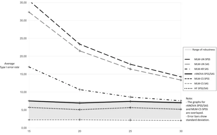
The results for nine measurement occasions under the condition of sphericity showed a progressive bias for MLM-UN and small sample sizes (Fig. 1).

Type I error inflation was higher for MLM-UN per-formed in SPSS compared to MLM-UN in SAS. Mul-tilevel linear models with compound symmetry demonstrated a slightly better performance for SAS than for SPSS as the Type I error rates of MLM-CS SAS were closer to the 5 % level. The Kenward-Roger-correction for MLM-UN SAS reduced the Type I error rate but did not fully solve the issues of small sample sizes, especially for n = 25 or below. The uncorrected rANOVA showed the expected Type I error rates close to five per cent when the sphericity condition holds, regardless whether they were performed in SPSS or SAS and with or without Huynh-Feldt-correction. The results for nine

meas-urement occasions showed higher inflation in Type I error rates for MLM-UN when sphericity was vio-lated (Fig. 2). Again, this progressive bias turned out to be stronger for MLM-UN in SPSS than in SAS. The Kenward-Roger-correction results did not differ much from the Type I error rates of this method for nine measurement occasions under the sphericity

HAVERKAMP & BEAUDUCEL

8

condition (cf. Fig. 1). The Type I error rates for the uncorrected rANOVA in SPSS and SAS as well as for MLM-CS in SPSS did not differ substantially and showed a moderately inflated Type I error. The Huynh-Feldt correction provided satisfying results

of Type I error rates close to five per cent for both software packages, while MLM-CS shows a striking conservative bias when performed with SAS and a large difference to results for the same method when performed in SPSS.

Figure 2. Average Type I error rates for 5,000 tests: nine measurement occasions, sphericity violation.

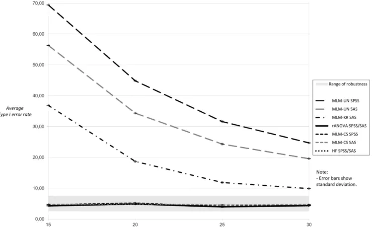
For twelve measurement occasions and no sphe-ricity violation, a large progressive bias for MLM-UN and small sample sizes emerged (Fig. 3; please note different scaling of the ordinate). Again, this Type I error inflation was higher for MLM-UN performed in SPSS compared to MLM-UN in SAS. The Ken-ward-Roger-correction for MLM-UN in SAS does

not solve the problem of Type I error inflation for n = 30 or below. The MLM-CS and rANOVA results showed Type I error rates close to five per cent, re-gardless whether they were performed in SPSS or SAS or – in case of rANOVA – with or without Huynh-Feldt-correction.

Figure 3. Average Type I error rates for 5,000 tests: twelve measurement occasions, sphericity assumption

holds.

When sphericity was violated, the results for twelve measurement occasions showed a similar high inflation in Type I error rates for MLM-UN as without violation (Fig. 4). As under the previous con-ditions, this progressive bias was stronger for MLM-UN in SPSS than in SAS. The Kenward-Roger-cor-rection results resemble the Type I error rates of

this method under the sphericity condition for 12 measurement occasions. The rates for the uncor-rected rANOVA in SPSS and SAS as well as for MLM-CS in SPSS appear similar and show an expected moderately inflated Type I error. Again, the Huynh-Feldt correction delivers Type I error rates close to five per cent for both software packages, while a conservative effect for MLM-CS was found for SAS.

HAVERKAMP & BEAUDUCEL

10

Figure 4. Average Type I error rates for 5,000 tests: twelve measurement occasions, sphericity violation.

Concluding the results section, a few findings concerning MLM-UN should be pointed out: The Type I error inflation for the uncorrected MLM-UN is remarkably high when sample sizes are small. This effect is so massive that it cannot be adequately cor-rected via the use of MLM-KR. On the other hand, the results show a trend where for both software packages the MLM-UN method shows less Type I error as the sample size increases. To investigate

whether a large sample size would lead to an ac-ceptable average Type I error rate, we performed an additional simulation using the same data from our main study only for all facets of MLM-UN (uncor-rected in SAS/SPSS, Kenward-Roger in SAS) for a sample size of n = 100 with twelve measurement oc-casions under the condition of sphericity (see Table 3).

Table 3

Average Type I error rates for different sample sizes and versions of MLM-UN

MLM-UN version n = 15 n = 30 n = 100

MLM-UN SAS 56,33 19,56 7,76

MLM-SAT SAS 56,33 19,56 7,76

MLM-KR SAS 36,87 9,86 5,66

MLM-UN SPSS 69,42 24,66 8,80

Table 3 shows the results of the additional simu-lation. Concerning our expectations, two conclu-sions can be drawn: First, the trend of uncorrected MLM-UN results to lower Type I error rates as sam-ple size increases can be confirmed. However, even for a large sample size of n = 100, the average Type I error rates of MLM-UN still failed to meet Bradley’s liberal criterion (Bradley, 1978) in SAS and SPSS. Only if MLM-UN results were corrected by means of MLM-KR, they showed no liberal bias in Type I error.

As the differences between SPSS and SAS for MLM-UN are considerable, we tried to examine how these disparities can be explained. First, we in-spected the underlying linear mixed model algo-rithms for SPSS (IBM Corporation, 2013) and SAS (SAS Institute Inc., n. d.) and found no differences. Second, we noticed indications for differences in the calculation of denominator degrees of freedom be-tween the MIXED procedures of SPSS and SAS in-cluding the advice to employ the Satterthwaite method to compute denominator degrees of free-dom in SAS if we “want to compare SAS results for mixed linear models to those from SPSS” (IBM Cor-poration, 2016) because it is reportedly used by de-fault in SPSS. To explore whether the heterogeneity between the MIXED Type I error rates of MLM-UN for SAS and SPSS can be explained by this difference, we also included the Satterthwaite method to cor-rect MLM-UN results (MLM-SAT) in our additional simulation in SAS as there is no option to alter the default method in SPSS (see Table 3). We would ex-pect similar average Type I error rates between MLM-SAT SAS and MLM-UN SPSS when the sup-posed differences in the calculation of denominator degrees are causal for the diverging simulation re-sults in MLM-UN. However, it turns out that it was not possible to reproduce the results of MLM-UN SPSS by employing the Satterthwaite method to compute denominator degrees of freedom in SAS because the results of MLM-SAT and MLM-UN SAS were nearly identical. It therefore remains an im-portant question for future research to explain these disparities between SAS and SPSS for suppos-edly identical methods in rather simple repeated measures data.

Discussion

As expected, we found that uncorrected ANOVA (rANOVA) and MLM-CS had 5% of Type-I errors at an alpha-level of 5% when they were used in data without violation of the sphericity assumption. The expected increase of Type-I error rates was also found for rANOVA and MLM-CS with data violating the sphericity assumption. Although we found the expected Type-I error rate of 5% for rANOVA-HF we found unexpected larger Type-I error rates for MLM-KR in data violating the sphericity assump-tion. The larger Type-I error rates for MLM-UN in small samples with and without violation of the sphericity assumption were again confirmed (Ken-ward & Roger, 1997, 2009; Haverkamp & Beauducel, 2017). As Kenward and Roger (1997) noted, the rea-son for bias of MLM-UN is probably that the preci-sion is obtained from an estimate of the variance-covariance matrix of its asymptotic distribution. However, in small samples, asymptotic-based measures of precision can overestimate the true precision. The results of our study thus confirm that asymptotic-based measures of precision can lead to biased results of MLM. Finally, unexpected differ-ences between MLM-UN SPSS and MLM-UN SAS as well as between MLM-CS SPSS and MLM-CS SAS occurred for the simple repeated measures data structure investigated.

The results of this simulation study bear some implications for the analysis of repeated measures designs in terms of best practice recommendations. Note that these suggestions are based on very basic designs as the simulated data contained no within-subject effect and neither a between-within-subjects nor a between-group effect. As pointed out before, we took these restrictions to examine Type I error rates for within-subject models that are not distorted in any way by the influences of other effects or levels.

The following implications for simple within-subject repeated measures designs can be derived from this simulation study:

1. The use of MLM-UN to analyze data with nine or more measurement occasions with samples com-prising 30 cases or less is generally not recom-mended without a correction method. This bias is stronger when MLM-UN is performed with SPSS.

HAVERKAMP & BEAUDUCEL

12

When MLM-UN has to be applied, it is best to use it with the Kenward-Roger correction (MLM- KR). If an uncorrected MLM-UN has to be the method of choice for some reason, estimation via SAS would be more appropriate than estimation via SPSS but would still result in huge inflation of Type I error if the sample size is small. Although there was more convergence between MLM-UN SPSS and MLM-UN SAS for a sample of about 100 participants, there was still a slightly smaller Type I error for SAS. Moreover, a small post-hoc simulation revealed that the differ-ences between MLM-UN SAS and MLM-UN SPSS cannot be accounted for by the Satterthwaite method for the correction of degrees of freedom, which is a non-default option in SAS and which is always used in SPSS.

2. According to the criterion of Bradley (1978), MLM-UN without correction showed a liberal bias under every simulated condition regardless of the software package. For twelve measurement occa-sions, the Kenward-Roger correction in SAS does not solve the problem of Type I error inflation for n = 30 or smaller. For nine measurement occasions, Kenward-Roger only delivers a result without a lib-eral bias if the sample size is above n = 25. The Ken-ward-Roger correction does, however, correct for some of the large liberal bias of uncorrected MLM-UN. If MLM-UN is required for the analysis of re-peated measures data that involves a high number of measurement occasions as well as a small sample size that is about n = 25 or larger, it is recommended to use it with the Kenward-Roger correction.

3. For nine measurement occasions, a conserva-tive bias according to Bradley (1978) was found for MLM-CS if sphericity was violated. This effect was specific to the SAS software package, as the MLM-CS results for SPSS showed no conservative bias but Type I error rates that were on the verge of the lib-eral criterion. These findings plead for the use of SPSS if MLM-CS has to be applied in spite of non-sphericity.

4. In accordance with previous research, the findings of this simulation study in general argue for the use of MLM-CS or rANOVA if the sphericity as-sumption holds as well as a correction of rANOVA results via the Huynh-Feldt correction if sphericity is violated. No major differences in the software packages occurred for the results of these methods. The encouraging results on rANOVA are in line with previous results on ANOVA when the assumption of

the normal distribution is violated (Schmider, Zieg-ler, Danay, Beyer, & Bühner, 2010).

There are, of course, several limitations to this study:

• The population data contained no within-sub-ject effect and neither a between-subwithin-sub-jects nor a be-tween-group effect and no interactions. Accord-ingly, the model was restricted to a simple within-subjects design.

• Not all methods, particularly corrections for MLM as Kenward-Roger, were available in both soft-ware packages. This is a limitation because we do not know how the Kenward-Roger correction would work in the context of the SPSS algorithm.

• SAS and SPSS do not provide a complete de-scription of their algorithms and they do not provide the software scripts. Therefore, the exact reasons for the differences could not be determined. Of course, the software packages are protected by law because people who develop the software scripts need to be paid for their work. However, when con-siderable differences between software packages occur even for rather simple data, the law protec-tion might constitute a limitaprotec-tion for the scientific value of the software.

Furthermore, this study yields some indications for future research:

• The examination of Type I error rates for the discussed methods should be expanded to more complex models including between-subject effects or between-within interaction effects.

• The differences in the results of very basic methods in statistical software packages have to be further explored, especially concerning MLM-UN and MLM-CS.

• The reasons of the massive Type I error inflation for MLM-UN at lower sample sizes have to be ana-lyzed in-depth. It may also be interesting to include R in further research in order to have at least one software where all the scripts are available.

In the course of the ongoing debate about the lack of reproducibility of scientific studies, different recommendations have been developed: Benjamin et al. (2017) proposed to set the statistical standards of evidence higher by shifting the threshold for de-fining statistical significance for new discoveries from p < 0.05 to p < 0.005. Lakens et al. (2017), on the other hand, formulate a more general demand of justifications of all key choices in research design and statistical practice to increase transparency.

We therefore see the results of this study as help-ful for researchers’ methodological choices when analyzing repeated measures designs: Only if the characteristics of different methods under specific conditions (e.g. their robustness against progressive bias when sample sizes are small or sphericity is vi-olated) are known, researchers can choose their method on the basis of this knowledge.

Open Science Practices

This article earned the Open Materials badge for making the materials available. It has been verified that the analysis reproduced the results presented in the article. The entire editorial process, including the open reviews, are published in the online sup-plement.

References

Arnau, J., Bono, R., & Vallejo, G. (2009). Analyzing Small Samples of Repeated Measures Data with the Mixed-Model Adjusted F Test.

Communica-tions in Statistics - Simulation and Computa-tion, 38(5), 1083–1103.

https://doi.org/10.1080/03610910902785746 Arnau, J., Balluerka, N., Bono, R., & Gorostiaga, A.

(2010). General linear mixed model for analys-ing longitudinal data in developmental re-search. Perceptual and Motor Skills, 110(2), 547– 566. https://doi.org/10.2466/PMS.110.2.547-566

Baayen, R. H., Davidson, D. J., & Bates, D. M. (2008). Mixed-effects modeling with crossed random effects for subjects and items. Journal of

Memory and Language, 59(4), 390–412.

https://doi.org/10.1016/j.jml.2007.12.005 Baek, E. K., & Ferron, J. M. (2013). Multilevel models

for multiple-baseline data: Modeling across-participant variation in autocorrelation and re-sidual variance. Behavior Research Methods,

45(1), 65–74.

https://doi.org/10.3758/s13428-012-0231-z

Benjamin, D., Berger, J., Johannesson, M., Nosek, B., Wagenmakers, E.-J., Berk, R., . . . Johnson, V. (2017). Redefine statistical significance. Berkhof, J., & Snijders, T. A. B. (2001). Variance

Component Testing in Multilevel Models.

Jour-nal of EducatioJour-nal and Behavioral Statistics, 26(2), 133–152.

https://doi.org/10.3102/10769986026002133 Boisgontier, M. P., & Cheval, B. (2016). The anova to mixed model transition. Neuroscience and

Bi-obehavioral Reviews, 68, 1004–1005.

https://doi.org/10.1016/j.neubio-rev.2016.05.034

Bradley, J. V. (1978). Robustness? British Journal of

Mathematical and Statistical Psychology, 31(2),

144–152. https://doi.org/10.1111/j.2044-8317.1978.tb00581.x

Ferron, J. M., Bell, B. A., Hess, M. R., Rendina-Go-bioff, G., & Hibbard, S. T. (2009). Making treat-ment effect inferences from multiple-baseline data: The utility of multilevel modeling ap-proaches. Behavior Research Methods, 41(2), 372–384.

https://doi.org/10.3758/BRM.41.2.372 Ferron, J. M., Farmer, J. L., & Owens, C. M. (2010).

Estimating individual treatment effects from multiple-baseline data: A Monte Carlo study of multilevel-modeling approaches. Behavior

Re-search Methods, 42(4), 930–943.

https://doi.org/10.3758/BRM.42.4.930

Field, A. (1998). A bluffer's guide to … sphericity. The

British Psychological Society: Mathematical, Statistical & Computing Section Newsletter, 6(1),

13–22.

Finch, W. H., Bolin, J. E., & Kelley, K. (2014).

Multi-level modeling using R. New York: CRC Press.

Goedert, K. M., Boston, R. C., & Barrett, A. M. (2013). Advancing the science of spatial neglect reha-bilitation: An improved statistical approach with mixed linear modeling. Frontiers in

Hu-man Neuroscience, 7, 211.

https://doi.org/10.3389/fnhum.2013.00211 Gomez, E. V., Schaalje, G. B., & Fellingham, G. W.

(2005). Performance of the Kenward–Roger Method when the Covariance Structure is Se-lected Using AIC and BIC. Communications in

Statistics - Simulation and Computation, 34(2),

377–392. https://doi.org/10.1081/SAC-200055719

HAVERKAMP & BEAUDUCEL

14

Gueorguieva, R., & Krystal, J. H. (2004). Move over ANOVA: Progress in analyzing repeated-measures data and its reflection in papers pub-lished in the Archives of General Psychiatry.

Archives of General Psychiatry, 61(3), 310–317.

https://doi.org/10.1001/archpsyc.61.3.310 Haverkamp, N., & Beauducel, A. (2017). Violation of

the Sphericity Assumption and Its Effect on Type-I Error Rates in Repeated Measures ANOVA and Multi-Level Linear Models (MLM).

Frontiers in Psychology, 8, 1841.

https://doi.org/10.3389/fpsyg.2017.01841 IBM Corporation. (2013). IBM Knowledge Center.

Model (linear mixed models algorithms).

Re-trieved September 7, 2018, from

https://www.ibm.com/support/knowledge- center/en/SSLVMB_22.0.0/com.ibm.spss.sta-tistics.algorithms/alg_mixed_model.htm IBM Corporation. (2016, September 07). IBM

Sup-port. Denominator degrees of freedom for fixed effects in SPSS MIXED. Retrieved September 7,

2018, from http://www-01.ibm.com/sup-port/docview.wss?uid=swg21477296

Kenward, M. G., & Roger, J. H. (1997). Small Sample Inference for Fixed Effects from Restricted Maximum Likelihood. Biometrics, 53(3), 983. https://doi.org/10.2307/2533558

Kenward, M. G., & Roger, J. H. (2009). An improved approximation to the precision of fixed effects from restricted maximum likelihood.

Computa-tional Statistics & Data Analysis, 53(7), 2583–

2595.

https://doi.org/10.1016/j.csda.2008.12.013 Keselman, H. J., Algina, J., Kowalchuk, R. K., &

Wolf-inger, R. D. (1999). A comparison of recent ap-proaches to the analysis of repeated measure-ments. British Journal of Mathematical and

Sta-tistical Psychology, 52(1), 63–78.

https://doi.org/10.1348/000711099158964 Knuth, D. E. (1981). The Art Of Computer

Program-ming: Seminumerical Algorithms (2. ed., 25.

print). Addison-Wesley series in computer

sci-ence and information processing: / Donald E. Knuth ; Vol. 2. Reading, Mass.: Addison-Wesley.

Kowalchuk, R. K., Keselman, H. J., Algina, J., & Wolf-inger, R. D. (2004). The Analysis of Repeated Measurements with Mixed-Model Adjusted F

Tests. Educational and Psychological

Measure-ment, 64(2), 224–242.

https://doi.org/10.1177/0013164403260196 Lakens, D., Adolfi, F., Albers, C., Anvari, F., Apps, M.,

Argamon, S., . . . Zwaan, R. (2017). Justify Your

Alpha.

Maas, C. J. M., & Hox, J. J. (2005). Sufficient Sample Sizes for Multilevel Modeling. Methodology, 1(3), 86–92.

https://doi.org/10.1027/1614-2241.1.3.86

McNeish, D. (2016). On Using Bayesian Methods to Address Small Sample Problems. Structural

Equation Modeling: a Multidisciplinary Journal, 23(5), 750–773.

https://doi.org/10.1080/10705511.2016.118654 9

McNeish, D. (2017). Small Sample Methods for Mul-tilevel Modeling: A Colloquial Elucidation of REML and the Kenward-Roger Correction.

Multivariate Behavioral Research, 52(5), 661–

670.

https://doi.org/10.1080/00273171.2017.134453 8

McNeish, D. M., & Stapleton, L. M. (2016a). The Ef-fect of Small Sample Size on Two-Level Model Estimates: A Review and Illustration.

Educa-tional Psychology Review, 28(2), 295–314.

https://doi.org/10.1007/s10648-014-9287-x McNeish, D. M., & Stapleton, L. M. (2016b).

Model-ing Clustered Data with Very Few Clusters.

Multivariate Behavioral Research, 51(4), 495–

518.

https://doi.org/10.1080/00273171.2016.116700 8

Nagelkerke, E., Oberski, D. L., & Vermunt, J. K. (2016). Power and Type I Error of Local Fit Sta-tistics in Multilevel Latent Class Analysis.

Structural Equation Modeling: a Multidiscipli-nary Journal, 24(2), 216–229.

https://doi.org/10.1080/10705511.2016.125063 9

Paccagnella, O. (2011). Sample Size and Accuracy of Estimates in Multilevel Models. Methodology,

7(3), 111–120.

https://doi.org/10.1027/1614-2241/a000029

SAS Institute Inc. (n. d.). SAS/STAT(R) 14.1 User's

Guide, Second Edition. Retrieved September 7,

http://support.sas.com/documen- tation/cdl/en/statug/68162/HTML/de- fault/viewer.htm#statug_mixed_over-view02.htm

Satterthwaite, F. E. (1946). An Approximate Distri-bution of Estimates of Variance Components.

Biometrics Bulletin, 2(6), 110.

https://doi.org/10.2307/3002019

Schmider, E., Ziegler, M., Danay, E., Beyer, L., & Bühner, M. (2010). Is It Really Robust?

Method-ology, 6(4), 147–151.

https://doi.org/10.1027/1614-2241/a000016 Snook, S. C., & Gorsuch, R. L. (1989). Component

analysis versus common factor analysis: A Monte Carlo study. Psychological Bulletin,

106(1), 148–154.

https://doi.org/10.1037/0033-2909.106.1.148

Tabachnick, B. G., & Fidell, L. S. (2013). Using

multi-variate statistics (6. ed.). Boston: Pearson

Edu-cation.

Usami, S. (2014). A convenient method and numeri-cal tables for sample size determination in lon-gitudinal-experimental research using multi-level models. Behavior Research Methods, 46(4), 1207–1219. https://doi.org/10.3758/s13428-013-0432-0

West, B. T., Welch, K. B., & Galecki, A. T. (2007).

Lin-ear mixed models: A practical guide using statis-tical software. Boca Raton Fla. u.a.: Chapman &