Research
2010:18
Radionuclide Transport: Preparation
During 2009 for the SR-Site Review
Authors: Peter RobinsonPhilip Maul Claire Watson
Title: Radionuclide Transport: Preparation During 2009 for the SR-Site Review. Report number: 2010:18
Author: Peter Robinson, Philip Maul and Claire Watson Quintessa Ltd. UK
Date: December 2009
This report concerns a study which has been conducted for the Swedish Radiation Safety Authority, SSM. The conclusions and viewpoints presented in the report are those of the author/authors and do not necessarily coincide with those of the SSM.
SSM Perspective
Background
Post-closure safety assessments for nuclear waste repositories involve radioecological modelling for an underground source term. Following several decades of research and development, the Swedish Nuclear Waste Management Company (SKB) is approaching a phase of license application. According to SKB’s plans, an application to construct a geological repository will be submitted by the end of 2010. The applica-tion will be supported by a post-closure safety assessment. In order to prepare for the review of the oncoming license application the Swedish Radiation Safety Authority (SSM), has performed research and develop-ment projects in the area of performance assessdevelop-ment (PA) modelling during recent years. Independent modelling teams have been establis-hed, including both “in house” as well as consultant’s competences. Quintessa have undertaken research and development for the Swedish re-gulatory authorities over many years. This has included the development of approaches and models for consequence analysis (radionuclide trans-port) that can be used to support the review of submissions from SKB.
Objectives of the project
SSM held a workshop at Rånäs Castle from 18 – 20 February 2009 to discuss the status of Consequence Analysis capabilities and to plan for preparatory work in the current year. Out of this meeting and subse-quent discussions, four areas were identified where further research during 2009 would be beneficial:
1. spatially varying transport properties;
2. choices of PDFs (probability density functions) and parameter correlations;
3. SKB’s approach to quantifying the role of the various barriers; and 4. combining scenarios.
This report documents the research that was undertaken.
Project information
Project manager: Shulan Xu
Project reference: SSM 2009/2090 Project number: 1692
Summary
SSM held a workshop at Rånäs Castle in February 2009 to discuss the status of Consequence Analysis capabilities and to plan for preparatory work in the current year. Out of this meeting and subsequent discussions, four areas were identified where further research during 2009 would be beneficial:
spatially varying transport properties;
choices of PDFs (probability density functions) and parameter correlations;
combining scenarios; and
SKB‟s approach to quantifying the role of the various barriers.
This report documents the research that was undertaken.
The most important findings for consequence analysis and the conduct of the SR Site review are listed here.
In the study of spatially varying properties, the following conclusions were made.
The SKB F-factor approach is exact only in the case of a single nuclide, constant
matrix properties and no dispersion. Compared to other sensitivities, the effect of dispersion for Peclet numbers 10 and higher is small.
Output fluxes are highly sensitive to the F-factor itself, but not to the water travel
time. Matrix penetration depth can be important if it is small, (less than about 10 cm in the cases considered here). The retention and porosity in the matrix have a direct proportional effect on peak releases for the single sorbed nuclide.
Varying matrix retention properties along a flow path can be handled exactly for a
single nuclide, a result that SKB may be unaware of.
The main approximation that can occur with the F-factor approach is in the use of
constant matrix retention properties for a chain case. When there are short-lived daughters, their output fluxes are strongly influenced by the matrix retention properties at the end of the path rather than by any overall average.
Cases using path lines generated using SSM‟s independent discrete feature model
showed that the EDZ can dominate the F-factor for many release points. In such cases, the properties of this EDZ control the output flux. The approach that SKB take to the EDZ in SR Site should be a focus for review. The relevance of such
issues will depend on which canister failure scenarios are considered – if failures can only occur by buffer erosion then this is likely to be where flows are at their highest and path lines from such location may not pass through the EDZ.
For the study of PDFs, key parameters have been reviewed for the source-term, near-field and geosphere. The following conclusions were reached.
A key issue for the release overall is the resistance of the buffer-fracture interface.
The importance of this process is well-known and must continue to be a focus for the review. It is more important than the transport resistance offered by the buffer as a diffusive barrier. In particular, results are rather insensitive to details of the near-field sorption properties.
Of the near-field parameters, the initial release fractions (IRFs) had the biggest
impact on the result; using the alternative conservative values resulted in an order of magnitude increase in the peak dose (both near-field and total).
Fuel dissolution rates are significant for later releases. Near-field doses are more
sensitive to the fuel dissolution rate distributions than to solubility limit distributions.
The use of uncorrelated radionuclide solubilities had no discernable effect on the
dose; and the use of sorption coefficients for bentonite in saline and non-saline groundwaters caused approximately a factor of 2 reduction in the peak dose.
In the far-field, the uncertainty is likely to be dominated by conceptual model
uncertainty (e.g. different discrete feature models) leading to different flow distributions.
The effects of reducing the matrix Kd value for Ra were considered for both a small and a sampled (effectively infinite) matrix penetration depth. In both cases the smaller sorption coefficient led to a smaller total dose.
The SKB calculations for the role of the various barriers presented in SR-Can have been satisfactorily reproduced, confirming that the basis for these calculations is adequately understood. In particular, the following conclusions were reached.
The calculations emphasise the key role played by the copper shells in SKB‟s safety case, but this depends on the calculated slow rate of copper corrosion in repository conditions.
As previously documented, the role of the buffer as a barrier to radionuclide
the transport resistance of the buffer neglected; a case with no buffer would behave very differently.
With other barriers in place radionuclide retention in the geosphere is less
important than other barriers, but when other barriers fail, this can be important in keeping calculated consequences to levels that are comparable with background radiation. In these cases, modelling of fuel dissolution can become much more important.
Looking at the impact of combined scenarios, the following conclusion was reached.
A combined pinhole and erosion scenario could give spike releases of a factor 3
Contents
1 Introduction 1
2 Previous AMBER and QPAC-TRAN Calculations 2
2.1 The SR-Can Calculations ... 2
2.2 Additional Calculations undertaken in 2008 ... 7
2.3 Current Knowledge on Important Features of the PA ... 8
3 Spatially Varying Transport Properties 9 3.1 Introduction ... 9
3.2 The SKB Approach and Justification ... 9
3.3 Mathematical Basis ... 12
3.4 Numerical Study into Varying Properties ... 22
3.5 Examples Using Pathlines ... 43
3.6 Conclusions ... 50
4 PDFs and Parameter Correlations 52 4.1 Introduction ... 52
4.2 Triangular and Log-triangular PDFs ... 53
4.3 Correlated Quantities ... 53
4.4 Review of SKB Choices and Assumptions ... 54
4.5 Additional Calculations ... 61
4.6 Conclusions ... 75
5 Quantifying the Role of the Different Barriers 76 5.1 Introduction ... 76 5.2 No Copper Shells ... 77 5.3 No Canisters ... 78 5.4 No Buffer ... 78 5.5 No Canisters or Buffer ... 78 5.6 Conclusions ... 79 6 Combining Scenarios 80 7 Conclusions 82 References 84 Appendix A Nomenclature 86
1
Introduction
Quintessa have undertaken research and development for the Swedish regulatory authorities over many years. This has included the development of approaches and models for consequence analysis (radionuclide transport) that can be used to support the review of submissions from SKB. Independent calculations in support of the regulatory review of SKB‟s SR-Can assessment (SKB, 2006, henceforth referred to as the SR-Can main report) using the AMBER software are described in Maul et al. (2008). Further work undertaken in 2008 was reported by Maul and Robinson (2008); this included the use of software based on Quintessa‟s general purpose modelling code QPAC, referred to as QPAC-TRAN.
With the expected submission of SKB‟s SR-Site documentation in support of a licence application at the end of 2010, the focus for consequence analysis in 2009 has been further preparation for SSM‟s review.
SSM held a workshop (Wilmot, 2009) at Rånäs Castle from 18 – 20 February 2009 to discuss the status of Consequence Analysis capabilities and to plan for preparatory work in the current year. Out of this meeting and subsequent discussions, four areas were identified where further research during 2009 would be beneficial:
1. spatially varying transport properties;
2. choices of PDFs (probability density functions) and parameter correlations; 3. SKB‟s approach to quantifying the role of the various barriers; and
4. combining scenarios.
This report documents the research that was undertaken.
In Section 2 some previously undertaken radionuclide transport calculations relevant to the present work are summarised. Progress in each of the four technical areas is discussed in turn in Sections 3 to 6. Section 7 brings together some conclusions.
2
Previous AMBER and QPAC-TRAN
Calculations
2.1
The SR-Can Calculations
Maul et al. (2008) described two types of calculation, mainly using the AMBER code: calculations aimed at reproducing SKB‟s radionuclide transport calculations, and calculations using independent geosphere data. The first set of calculations is most relevant for the topics considered in the present report.
2.1.1
The Pinhole Failure Mode
The Pinhole Failure mode is not considered likely to occur by SKB, but it has been studied in detail in previous assessments (including SR-97) and provided information that is relevant to calculations for other potential failure modes. In effect the pinhole failure mode provided a „reference‟ set of calculations.
Figure 1 gives details of the modelling blocks used in the near field, some of which are broken down into a number of compartments. The pathway Q4 was not considered by SKB in the SR-Can assessment, as it was assumed to be less important than the other pathways.
Figure 1: Discretisation of the Near Field
B 7 B 6 B 5 B 8 B 9 B 4 B 3 Q 1 Q 2 Q 3 Q 4
Some of the issues noted in implementing the SKB model in AMBER included:
Some of the flow resistances were defined as the reciprocal of equivalent flow
rates. Due to lack of clarity in the SKB documentation it was not clear whether the
AMBER implementation was totally compatible with the calculations presented in SR-Can, particularly for the Q3 pathway.
It is understood that the diffusive transport resistance at the buffer/rock interface
was neglected by SKB when spalling takes place, although it was not clear why this was considered to be appropriate.
Advective flows were included in the tunnel (only diffusive flows were included
in the Quintessa SR-97 Case File). The details of the parameter values used by SKB to represent this process were not totally clear from the SR-Can documentation, so it is not clear whether the approach taken in the AMBER implementation mirrored that employed by SKB.
SKB used data 'triples' for the correlated parameters F, tw and Qeq . Sample files proved by SKB were used directly for probabilistic calculations. It is understood that the data in these sample files did not include a factor of 10 division referred to on page 407 of the main SR-Can report (SKB, 2006a) to account for channelling effects.
SKB used correlated sorption coefficients. Values of Kd for elements (in a given redox state) in the same correlation group are correlated. The way that these correlations were implemented was not stated explicitly in the SR-Can documentation.
The following simplifications were made in the AMBER implementation:
1. The same geosphere transport parameters were taken for each of the transport pathways Q1, Q2 and Q3 when all the pathways are considered together. Alternatively, each pathway could be considered separately. To provide different geosphere parameters for the different pathways would require significant changes to the structure of the AMBER model. This issue can be addressed using QPAC-TRAN.
2. Reducing conditions were assumed throughout, and this determined the chemical form assumed for some elements that can be in more than one redox state.
The deterministic calculations presented by SKB were for Forsmark. Other than the biosphere dose factors, the only parameters that would differ between the two sites
would be the matrix porosity in the geosphere and the formation factors used in the calculation of effective diffusivities in the rock matrix. These differences are small, and so separate AMBER calculations were not been undertaken for Laxemar. Subsequently, Forsmark was chosen as SKB‟s preferred site.
Good agreement was obtained between the AMBER and SKB deterministic and probabilistic calculations, although some uncertainties remained because of the shortcomings in the SKB documentation and because associated deterministic calculations were not presented for each of the probabilistic calculations considered. Because these calculations for Forsmark are later taken as ‟reference‟ calculations, the probabilistic calculations with a log-triangular distribution for the fuel dissolution rate are summarised here.
Figure 2 shows AMBER probabilistic calculations obtained with 4000 samples with just pathway Q1 modelled. The run time for such calculations is about two days. This figure can be compared with Figure 10-20 in the SR-Can main report. The overall features are very similar for times up to about 104 y, but at longer timescales the
AMBER values for the mean and 99th percentile are around an order of magnitude
higher than the SR-Can values.
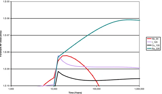
Figure 3 shows the contribution to the mean dose from the key radionuclides. This figure compares well with Figure 10-18 in the SR-Can main report, although the doses from Ra-226 and Pb-210 are somewhat higher at long times. The Pb-210 dose calculated by AMBER is not obtained in the SR-Can calculations because SKB do not model this radionuclide in the near field and geosphere; it is not clear that this will necessarily be an appropriate approximation for all possible parameter values in probabilistic calculations.
In Figure 10-19 of the SR-Can main report SKB gives dose calculations based on fluxes from the near field. Corresponding AMBER calculations are given in Figure 4, and the results compare very closely.
Figure 2: AMBER Probabilistic Calculations for Biosphere Doses for Forsmark 1.E-10 1.E-09 1.E-08 1.E-07 1.E-06 1.E-05 1000 10000 100000 1000000 Time (years) F o rs m a rk B io s p h e re D o s e ( S v /y ) 95% 99% Mean
Figure 3: AMBER Probabilistic Calculations for Biosphere Doses for Forsmark - Key Radionuclides 1.E-10 1.E-09 1.E-08 1.E-07 1.E-06 1.E-05 1,000 10,000 100,000 1,000,000 Tim e (Years) F o rs m a rk B io s p h e re D o s e s ( S v /y ) I_129 Cs_135 Pb_210 Ra_226
Figure 4: AMBER Probabilistic Calculations for “Near Field Doses” for Forsmark for Pathway Q1 1.E-10 1.E-09 1.E-08 1.E-07 1.E-06 1.E-05 1,000 10,000 100,000 1,000,000 Time (Years) F o rsmar k NF Do se ( S v/y ) Nb_94 I_129 Cs_135 Ra_226
2.1.2
The Lost Buffer Failure Mode
In this failure mode the canister was assumed to fail at a specified time and there was then an additional delay before the resistance to radionuclide transport from the canister is assumed to fall to zero. The calculations for this failure mode were actually much simpler and quicker to reproduce in AMBER than for the pinhole failure mode because there is no radionuclide transport in the buffer.
The following issues arose in comparing the AMBER and SKB calculations:
SKB spread the period over which the instantaneous release fractions for Ni-59
and Nb-94 left the canister once failure occurred. This change was not reproduced in the AMBER calculations.
The calculations reported in the main SR-Can report were for a high equivalent
flow rate, Qeq, although this was not made clear in the documentation, and no value was given.
Figure 10-41 of the SR-Can report gives modified (analytical) calculations with Th
retained in the canister, and these were compared with the full numerical calculation in Figure B-1 of the same report. SKB indicated in Section 10.6.5 of the SR-Can report that radionuclide in-growth was not included for this failure mode
(although it is not clear why). As a result, if co-precipitation of Th occurs in the canister, more Ra-226 will be released. This is an example of where it is not straightforward to identify conservative assumptions in systems as complex as the one being modelled here. Effectively reducing the solubility of Th results in higher doses, which may not necessarily have been expected. AMBER calculations were undertaken where the solubility of all Th isotopes was reduced to effectively zero and the resulting calculations were similar, but not identical to the SKB calculations.
Based on the discussion given in Appendix B of the SR-Can main report, it appears
that SKB‟s probabilistic calculations for the lost buffer failure mode used the alternative model where Th-230 is retained in the canister, but this was not totally clear.
The risks calculated from this failure mode depend critically on two key inputs:
the specified canister failure times and the assumed fuel dissolution rate. The first failure time calculated by SKB was not until nearly 500, 000 years at Forsmark. By this time most of the original inventory has decayed, and this is the main reason why the calculated risks are compatible with the relevant regulatory criterion.
2.1.3
Mechanical Failure Modes
Two such modes were considered by SKB. AMBER calculations were not undertaken to reproduce the SR-Can calculations for the Shear Movement failure, because it was considered that little additional insight would be gained beyond that obtained for the pinhole and advective failure modes; the risk calculations depend primarily on the probabilities assumed for the event happening.
Similarly, the consequences of the Isostatic Load failure mode can be assessed from the calculations produced for the pinhole failure mode, so no additional AMBER calculations were undertaken.
2.2
Additional Calculations undertaken in 2008
The developments described by Maul and Robinson (2008) included:
The use of the Quintessa‟s QPAC code with a radionuclide transport module
(referred to as QPAC-TRAN). QPAC is able to represent a wider range of transport processes than is possible with AMBER and this broadens the range of issues that can be addressed. One important assumption in this module is that the interface area between two compartments is taken to be the area that is actually in common for the relevant faces of the compartments. This is considered to be the
most physically-appropriate assumption, but does not correspond to that employed in the SR-Can assessment (and the AMBER calculations that reproduced these calculations) where a transport resistance approach was used with the net resistance being taken to be the average for the two compartments; this can imply a different effective interface area from that employed in QPAC-TRAN, and this resulted in small differences between AMBER and QPAC-TRAN calculations.
An improved approach to discretisation in the geosphere was described which
should improve the accuracy of radionuclide transport calculations and reduce computing run times.
AMBER remains a convenient and powerful tool for many types of calculation, particularly where probabilistic calculations are required. It is anticipated, however, that the wider range of problems that can be addressed using codes based on QPAC, and the flexibility provided by the use of file-based input, will mean that this will increasingly be used for addressing detailed radionuclide transport issues.
2.3
Current Knowledge on Important Features of
the PA
From the work described above and published work by, for example, Hedin (2003) the following key features of the performance of the KBS3_V are well understood:
Once canister corrosion has taken place the transport of radionuclides into the
geosphere is critically dependent on the characteristics of the buffer/rock interface; this is much more important than the characteristics of the buffer itself, such as bentonite sorption coefficients.
The rate of transport through the geosphere depends critically on the conceptual
model for the processes involved, particularly for the sorption of long-lived radionuclides in the rock matrix; very different results can be obtained with different models.
These topics are not the focus of the current work, but sensitivity to the buffer/rock interface transport resistance is discussed in Section 4.4 and the question of sorption in the rock matrix is consider in Sections 3.4.5 and 4.4.
3
Spatially Varying Transport Properties
3.1
Introduction
SKB have used a one-dimensional transport modelling approach for many years and it is expected that this will continue to be their main approach in SR-Site. This approach follows path-lines, calculated in a flow code, from a deposition hole to the near-surface environment.
Transport along this path is governed by advection and dispersion, radioactive decay and ingrowth, equilibrium sorption and matrix diffusion. SKB have argued that the matrix diffusion effects can be parameterised through the single F factor (Elert et al, 2004). The argument supporting this claim is quite restricted in its scope – being valid only for transport through homogeneous matrix material with constant penetration depth (i.e. varying fracture apertures and flow velocities along the path are allowed but not varying matrix properties). There are, however, many cases where parts of the flow path are through different materials, e.g. tunnel infill and/or near-surface soil layers. In these cases, the level of inaccuracy in taking averaged properties and a single F value is unclear. With the possible use of the MARFA code (as yet undocumented) in SR-Site, SKB will have the capability to undertake the radionuclide transport calculations more accurately, but this will not be their main assessment route.
The purpose of this task was to look at the sensitivity of transport calculations to the assumptions underlying the use of the F-factor. This was done by looking at the basic assumptions that underlie the F factor concept and by comparing solutions using the F factor approach to those obtained by splitting a path into separate parts for the different materials that it travels through.
3.2
The SKB Approach and Justification
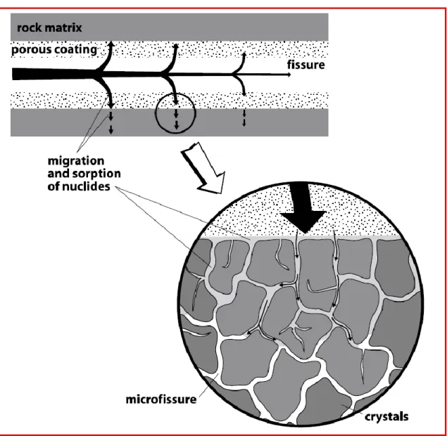
The approach used for radionuclide transport in the geosphere in SR-Can is summarised in Section 10.4.2 of the main SR-Can report (SKB, 2006a). This refers to the documentation for the FARF31 code (Elert et al, 2004) for details. Figure 5 shows the modelled system as depicted by Elert et al. A very similar figure appears in the SKI Project-90 report (SKI, 1991, Figure 4.8.1). The CRYSTAL code was developed by SKI to calculate one-dimensional transport in these systems (Worgan and Robinson, 1995).
Figure 5: Matrix diffusion in the micro-fissures in the rock matrix (from Elert, 2004)
It is stated by Elert et al (2004) that the DFN (discrete fracture network) calculations calculate the advective travel time (tw) and the transport resistance (F) and that FARF31 uses these inputs directly. The European RETROCK project (RETROCK, 2005) is quoted and provides a useful summary, noting that the Posiva and SKB definitions of F differ by a factor of 2. The F-factor is defined by SKB as the integral over time of the flow wetted surface (per unit volume of water) along the path line and hence has units of y m-1.
Limitations of the migration path concept are said to be that it is restricted to time-invariant flow fields and that “with the current utilisation of the F-factor integrated over the
migration path as an input parameter the solution is formally correct for single-member decay chains only. For longer decay chains, use of the integrated parameter F is strictly not correct if the channel width to flow ratio varies in space.”
The FARF31 report (Elert et al, 2004) gives the equations that are solved and indicates that averages are required along the path. It seems to take for granted that an appropriate average F value along the path can be calculated.
The SR-Can data report (SKB, 2006b) records how the F and tw parameters are calculated, but does not discuss the assumptions that underlie this. This report also makes it clear that parts of the flow path in the tunnels or EDZ are excluded from the calculation.
For a discussion of the underlying assumptions it is necessary to go back to Andersson et al (1998) and Selroos and Cvetkovic (1996).
Andersson et al (1998) clearly state that “for the simple case with no dispersion and matrix
diffusion into an infinite matrix … the sum of the F-quotients determines the transport as long as Dm,i [matrix diffusivity] and Kd,i [matrix sorption] are constant”. They go on to state that “In SR-97 this [the constant diffusion and matrix properties] will also be assumed to be the
case” but that “generally also Dm,i and Kd,i vary along the flow path and the proper averaging
must preserve the u value [a lumped parameter in the analytic solution] rather than the F-value”. Furthermore, “the extension is less straight-forward for cases with important dispersion in the fracture or a finite penetration depth”.
Selroos and Cvetkovic (1996) provide a more technical analysis but take the same approach (they denote the F-factor as
).Posiva have also adopted the F-factor approach, although they use the terminology WL/Q, where W is the fracture width (orthogonal to the flow), L is the path length and Q is the flow rate; this is equal to half of the F-factor as SKB would define it. A recent Posiva assessment (Smith et al, 2007) states that there has been no fundamental change in the Posiva approach since TILA-99.
In summary, the limitations of the F-factor approach were clear when it was first introduced. However, the approach is now used without comment for situations where these limitations are not respected. Although the approach may well remain a good approximation (particularly in the context of the uncertainties that exist in the precise values of the relevant geosphere properties) this has not been demonstrated. The purpose of the current work is to explore whether there are any significant errors that arise when using the F-factor approach for a general system.
In the following section, the governing equations are stated and some analytic results are derived to show where the F-factor arises and when it is valid to integrate along a flow path. Some numerical calculations are then performed to indicate the level of approximation that arises when the F-factor is used beyond where it is strictly valid.
3.3
Mathematical Basis
The various reports that have been referred to above all use slightly different notations. Here, we endeavour to define all the terms that we use as they are introduced and summarise them in a table in Appendix A.
We start by defining the general system of governing equations that we will consider. Simplified versions of these will then be considered.
3.3.1
The Full Set of Transport Equations
Conceptually, we consider transport along a one-dimensional flow tube. The water velocity along the flow tube can vary, but the total flow rate along the tube is constant. There is exchange between neighbouring flow paths which manifests itself as longitudinal dispersion within the flow tube of interest. Moreover, this exchange ensures a constant concentration across a fracture and each flow tube sees its share of the rock matrix surfaces for sorption and matrix diffusion. In practice this means that we can assume that the flow tube extends across the full aperture of each fracture but is of varying width, consistent with the local pore velocity in the fracture. We assume that the fractures are open and planar.
The governing equation for transport along the flow tube can then be written
0 1 1 1 2 2
z n m n m f n f n f n n f n f n n f n f n f n f n fdz
dC
D
C
R
C
R
x
C
v
x
C
D
t
C
R
(3.1) wheret is the time [y]
x is the distance along the flow tube [m] n
f
C is the concentration of nuclide n in the flowing water [moles/m3]
n f
R is the retardation (due to surface sorption if any) of nuclide n [-]
n f
D is the dispersion/diffusion coefficient for nuclide n. n
eff n f
D
Pe
vL
D
[m2/y]L is the path length [m]
n eff
D is the effective diffusion coefficient for nuclide n, which in an open fracture
would be equal to the pore water diffusion coeffcient [m2/year]
v is the water velocity [m/year] n
is the decay constant for nuclide n [per year] f
is the specific surface area of matrix (i.e. area per unit volume of flowing water) [m2/m3]n m
C
is the concentration of nuclide n in the matrix water [moles/m3]z is the distance into the rock matrix [m] n
m
D
is matrix effective diffusion coefficient for nuclide n [m2/y] .The retardation can be calculated from the sorption parameters, using n m a m f n f K R 1
(1
) , (3.2) where, m
is the matrix porosity [-] nm a
K , is the area-based sorption coefficient of nuclide n for the matrix
[m3/m2].
For a planar fracture, the specific surface area is simply derived from the aperture:
h
f2
(3.3) where,h is the fracture aperture [m].
Note that half-apertures are sometimes used in formulating these equations, with consequent changes by factors of 2. This is the source of the difference between SKB‟s and Posiva‟s definitions.
In general the parameters can be spatially varying.
Implicit in this formulation is the flow rate along the flow tube, Q [m3/y], from which
vh
Q
w
. (3.4)Within the rock matrix, a diffusion equation applies
1 1 1 2 2
n m n m m n n m n m m n n m n m n m n m mR
C
R
C
z
C
D
t
C
R
(3.5) where n mR
is the retention factor in the matrix of nuclide n [-]The matrix retention of nuclide n can be calculated from the sorption parameters, using n m d m m m n m
K
R
,)
1
(
1
, (3.6) where m
is the matrix grain density [kg/m3]n m d
K , is the matrix sorption coefficient of nuclide n [m3/kg].
To complete the equations initial and boundary conditions are required. Initially, all the concentrations are zero. The boundary conditions for the flow tube can take various forms, but we will assume that a flux is specified at x=0,
n in x n f n f n f
G
dx
dC
D
vC
hw
0 . (3.7) Here n inG
has units of mol/y. At the far end, L [m], either a zero concentration or zero gradient condition is assumed depending on the situation. No downstream condition is necessary if there is no diffusion or dispersion.For the matrix, the concentration at the fracture equals that of the flowing water
n f z n m C C 0 , (3.8)and there may be a limited penetration depth, am [m], for the diffusion where 0 am z n m dz dC , (3.9)
which becomes redundant if an infinite matrix is assumed, being replaced by a condition that the concentration tends to zero at infinity.
The result of interest is the flux at the far end of the path: L x n f n f n f n out
dx
dC
D
vC
hw
G
, (3.10)again with units of mol/y. Note that in practice the value of the total flow rate for the flow tube, Q, need not be specified. It cancels out because the equations are all linear and only fluxes are of interest.
3.3.2
Single Nuclide Advection with Constant Properties
and Infinite Matrix
In the case of a single nuclide, the ingrowth terms in (3.1) and (3.5) are irrelevant. Disregarding diffusion and dispersion in the flow tube makes (3.1) first order and leaves no place for a downstream boundary condition. Assuming constant properties simplifies the solution. The assumption of an infinite matrix makes the solution particularly simple and is the starting point for seeing where the F-factor arises.
Here, and in later sections, we shall use a Laplace Transform approach to solving the equations. This is the approach used in FARF31 by SKB. When it is necessary to produce time-domain solutions, we will use Talbot‟s algorithm (Talbot, 1979; Robinson and Maul, 1991) to invert the Laplace Transform. This is also used by FARF31 and provides an essentially exact result.
The Laplace transformed simplified equations are:
0
)
(
z m m f f f fdz
C
d
D
dx
C
d
v
C
s
R
, (3.11) 2 2)
(
dz
C
d
D
C
s
R
m m m m m
, (3.12)with boundary conditions
v
C
f xG
inhw
0 . (3.13)
Cm z0 Cf . (3.14)Here, the over bar denotes the Laplace Transform and s is the Laplace variable [y-1]
f x Lout
hw
v
C
G
. (3.10)Note that this system, without the decay term, is analogous to the problem of heat exchangers discussed by Carslaw and Jaeger (1959).
The solution for the transformed matrix concentration is simply z f m C e C , (3.15) where m m m
D
s
R
(
)
. (3.16)Substitution into (3.11) gives
dx C d v C D s Rf(
)
f m
f f . (3.17)The solution is then
Rf s fDm
v x in fe
hwv
G
C
( ) , (3.18)and the required result is
in f
f m
out R s D v L G G exp ( ) . (3.19)We can now relate this to the F-factor and advective travel time. In our notation, the F-factor is defined as
v L
F
f , (3.20)which corresponds to the formula given by SKB‟s SR-Can data report (SKB, 2006b, Section 6.6)
Q
wL
F
2
through the relationships given in (3.3) and (3.4).The travel time is given by SKB as
Q
hwL
t
w
which is simply equivalent tov
L
t
w
.This is valid if it is assumed that there is no surface sorption (
R
f
1
), but morev LR
tw f . (3.21)
Then, the required result can be written
w
m
in
out
G
t
s
FD
G
exp
(
)
. (3.22)If we take the case where the input is a pulse of unit strength, then the Laplace Transform can be explicitly inverted to give
)
(
)
(
4
exp
)
(
4
2 3 2 w w m m m w m m m t outH
t
t
t
t
D
R
F
t
t
D
R
F
e
G
. (3.23)Thus, the F-factor and tw represent the fracture-dependent part of the solution while the matrix contribution is a product of three key matrix properties. This result agrees with that quoted by Selroos (1996).
3.3.3
Single Nuclide Advection with Varying Fracture
Properties and Infinite Matrix
When the fracture properties vary it is clear from (3.22) that a summation (or integration) approach can be taken to deriving an F-factor and tw for the total path. In the case of piecwise-constant properties in N segments, the result simply becomes
m i i i wi in N i m i i w in out G t s FD G t s FD G exp ( ) exp ,( ) 1 , . (3.24)The result for a continuously varying property evidently turns the sums into integrals. Thus, the assumption that is made about deriving the F-factor as a sum over the path is correct when there is no variation in matrix properties, the matrix is infinite and there is no dispersion/diffusion along the flow path.
3.3.4
Single Nuclide Advection with a Finite Matrix
If the matrix penetration depth is finite, so that (3.9) applies, the Laplace transform solution given in (3.22) changes slightly. It becomes
(
)
tanh(
)
exp
w
m
m
in
out
G
t
s
FD
a
G
. (3.25)This change makes no difference to the validity of the derivations of the F-factor and tw for the total path; the approach remains valid as long as all the matrix properties are constant.
Note that this also indicates that other matrix geometries would not change the validity – for example cylindrical diffusion from narrow channels, since they have very similar forms of transform – with the tanh replaced by, for example, Bessel functions.
Although direct inversion of this result to the time domain is intractable, it is straightforward to calculate the mean transport time for a pulse input. This is calculated from the derivative of the exponent in (3.25), evaluated at s=0. The result is
tanh( ) sech ( )
2 0 2 0 0 0
m m m m m w mean a a a R F t t , (3.26) m m mD
R
0 . (3.27)This result can be useful in obtaining an indication of sensitivity to the various parameters.
3.3.5
Single Nuclide Advection with a Varying Matrix
Properties
If the matrix properties vary along the path then the approach as it stands cannot be valid. There is a need to define suitable average matrix properties.
For the infinite matrix case this can be done quite simply. We rewrite (3.22) to emphasise the dependence on the matrix properties
t s F s
G s D R F s t G G m w in m m m w in out
) ( exp ) ( exp . (3.28)where we have written
m
mRmDm as the only matrix property that is relevant. Then, for a series of paths with difference properties eachG
in equals the previousG
out and the exponents are added together. Thus, a suitable average
must satisfyi m n i i ave m F F , 1 ,
, (3.29)which implies that the F-factors act as weights in the averaging:
n i i i m n i i ave m F F 1 , 1 ,
. (3.30)With this definition of the average matrix properties the F-factor approach can still be used. The authors are not aware of this being exploited by SKB or similar organisations.
For a finite matrix, the requirement would be
s D a s F s D a s F i m i m i m i m n i i ave m ave m ave m ave m
, , , , 1 , , , , tanh tanh . (3.31)This would have to be satisfied for all values of s. This is impossible and the F-factor approach cannot therefore be extended to this case.
3.3.6
Dispersion
We now look at the effect of dispersion, starting by deriving the solution for the simplest case of a single nuclide, infinite matrix and constant properties.
When dispersion is present, a downstream boundary condition is required. Given that we expect the effects of dispersion to be small (i.e. transport in the fracture is dominantly advective), we take a zero gradient condition, so the resulting flux is purely advective at the boundary.
We write the solution in a form that makes the connection with the non-dispersive case clear. We assume no diffusion in the fracture and use the Peclet number to characterise the degree of dispersion; a high Peclet number indicates advective dominance (assuming that diffusion along the flow path is negligible).
To this end, define
adv
t
w
(
s
)
FD
m . (3.32) so that
adv
in outG
G
exp
. (3.33)Then the solution with dispersion can be written as
in adv Pe oute
G
G
)
1
(
)
1
(
)
1
(
1
2
exp
, (3.34) wherePe
adv/
4
1
. (3.35)Clearly
1
as Pe and the advective result is recovered. Clearly, the F-factorapproach becomes invalid in the dispersive case, but can be expected to remain a good approximation for high Peclet numbers. Numerical experiments will quantify this. An additional complication in the dispersive case is that continuity conditions are needed between each segment in a case with piecewise constant properties. The effect of these is to make the solution dependent on the order in which the segments arise. This means that it is not strictly valid to group segments that have common properties together unless they actually occur contiguously in the flow tube, as would be natural for the non-dispersive case; the effect of this will also be explored through numerical experiments.
3.3.7
Chain Decay in the Advection Case
We now look at the effect of decay chains.
We first note that cases where all members of a chain share the same transport properties can be treated as single nuclide cases, since the total concentration can be modelled and then the distribution between members applied retrospectively from solution of the Bateman equations for decay and ingrowth (Bateman, 1910). Therefore, we are interested in the general case when the chain members have different properties.
In the general case the solution becomes mathematically much more complicated, with the result for each member depending on the behaviour of all previous chain members. The solution for the first member is, of course, identical to the single nuclide case. The general case is dealt with in Appendix B.
Here we start by exploring the solution for the simplest case of a 2-member chain with an infinite matrix and constant properties. The result for the first member is unchanged:
(1) (1) (1) (1)
) 1 ( ) 1 ()
(
exp
w
m
in outG
t
s
FD
G
. (3.36)The second member result can be written as a sum over the basic single-nuclide response. Specifically,
(1) (1) (1) (1)
21 ) 2 ( ) 2 ( ) 2 ( ) 2 ( 22 ) 2 ()
(
exp
)
(
exp
m w m w outFD
s
t
K
FD
s
t
K
G
, (3.37) where
(
)
(
)
.
)
(
)
(
) 1 ( ) 1 ( ) 1 ( ) 2 ( ) 2 ( ) 2 ( ) 1 ( ) 1 ( 21 ) 1 ( ) 1 ( ) 1 ( ) 1 ( ) 2 ( ) 2 ( ) 2 ( ) 2 ( ) 1 ( ) 2 ( 21 ) 2 ( ) 1 ( ) 1 ( 21 21 ) 2 ( 22s
R
D
D
s
R
R
U
D
s
R
D
s
R
U
D
R
K
K
G
K
m m m m m m f f m f f m f f in
(3.38)The later member results are better written in terms of recurrence relations, see Appendix B.
Thus, although the F-factor and tw still appear in these results, the introduction of chain decay causes complex coefficients to arise containing all the different properties. It is clear that the summation of F-factors will not be strictly valid for decay chains, even in the simplest case of an infinite matrix and only advection in the fracture. Moreover, no suitable average matrix properties can be derived.
The analytic form does not make it easy to see how big an error in the breakthrough for later chain members is likely to be made if the F-factor approach is used. Section 3.4.6 examines this by by numerical experiment.
Also note that decay chain results depend on the ordering of the segments. This arises because the solution involves a product of matrices that are non-commutative.
3.3.8
Summary
The F-factor approach as used by SKB can be seen to be fully mathematically valid for advective transport of a single nuclide with constant matrix properties. This applies to both finite and infinite matrix diffusion.
If the matrix properties vary then a suitable averaging scheme exists for the case of infinite matrix diffusion, but it is not thought that SKB have exploited this. In cases of interest the matrix penetration depth may be sufficiently large for the infinite case to be an excellent approximation.
For decay chain members whose breakthroughs are significantly affected by ingrowth from precursor nuclides, the F-factor approach is invalid. If all chain members share the same transport properties then the approach would be valid, so it is to be expected that the approximation will be poorest when there are significantly different properties (sorption being the most likely case). The quality of the approximation may depend on the ordering of segments, this will be investigated numerically.
Similarly, when dispersion is present the F-factor approach fails. The approximation will become increasing poor as the level of dispersion increases. SKB use a fixed Peclet number of 10; numerical experiments are required to determine whether this is large enough to make the F-factor approach sufficiently accurate. There is potential for the order in which properties are encountered to be significant in in the dispersive case; this needs to be investigated numerically.
3.4
Numerical Study into Varying Properties
In this section the various issues that have been identified are explored numerically. A computer code was developed to calculate the solution for the general case, using the Laplace transform approach that is used by SKB in FARF31 based on Talbot‟s algorithm (Talbot, 1979). Talbot‟s algorithm uses a simple sum over the Laplace transform values along a contour in the complex plane to provide highly accurate approximations to the original time-domain function. The implementation was tested using transforms with known inverses. The same algorithm was used in the CRYSTAL code (Worgan and Robinson, 1995) and is used by SKB in FARF31.
The objective is first to confirm that the F factor approach is exactly valid in some cases and to explore the level of approximation that is introduced when it is used in other situations.
To this end we start with a set of base cases from which variants will be derived.
3.4.1
Base Cases
The base cases share the same flow and geometry, differing only in the nuclides involved. The three cases are for: a non-sorbed nuclide (I129); a sorbed nuclide (Se79) and a decay chain (Np237, U233, Th229). The base cases are for a single segment with advection only. A source term is used that injects 1 mol of the parent nuclide over a short period using a leaching source term with a leach rate of 1 per year.
The flux out of the end of the system is reported.
In the parameter tables F-value and travel time, tw, are given along with physical properties (path length, velocity and aperture) that could lead to these values. From the analysis already presented it is clear that other values of the physical properties that correspond to the same F-value and travel time would give the same flux out of the system.
The parameters used for the base cases are given in Table 1and Table 2.
Table 1: Nuclide-independent Parameters for the Base Cases
Parameter Value Units
Path length 500 m
Flow velocity 10 m/y
Aperture 0.002 m
F value 50 000 y/m
Travel time 50 y
Peclet number Infinite (advection only) -
Rock porosity 0.001 -
Rock effective diffusion 6e-7 m2/y
Maximum penetration depth 0.03 m
Source leach rate 1 y-1
Table 2: Nuclide-independent Parameters for the Base Cases
Parameter I129 Se79 Np237 U233 Th229 Units
Decay constant 4.415e-8 1.84e-6 3.24e-7 4.36e-6 9.44e-5 y-1
Rock retention factor 1 2e3 2e5 1e6 2e5 -
Figure 6: Flux output for I129 Base Case 0 0.05 0.1 0.15 0.2 0.25 0.3 0.35 50 52 54 56 58 60 62 64 66 68 70 Time (years) F lu x (mo l/ y)
Figure 7: Flux output for Se79 Base Case
0.0E+00 5.0E-05 1.0E-04 1.5E-04 2.0E-04 2.5E-04 3.0E-04 3.5E-04 0 1000 2000 3000 4000 5000 6000 7000 8000 9000 10000 Time (years) F lu x (mo l/ y)
Figure 8: Flux output for Np237 Chain Base Case 1.E-10 1.E-09 1.E-08 1.E-07 1.E-06 1.E-05
0.E+00 1.E+05 2.E+05 3.E+05 4.E+05 5.E+05 6.E+05 7.E+05 8.E+05 9.E+05 1.E+06
Time (years) F lu x (mo l/ y) Np237 U233 Th229
The I129 result shows a very rapid peak after the travel time of 50 years, indicating that the matrix diffusion has a very small effect.
The Se79 results show a peak after around 550 years; the shape of the curve is characteristic of a matrix diffusion case with the slowly falling flux after the initial peak caused by diffusion out of the matrix.
The Np237 chain result shows a peak for Np237 around 50000 years with the shape of the curve similar to the Se79 case. The daughter nuclides grow in during transport of the parent and show a later peak; the shorter-lived Th229 is in equilibrium with the U233 and the ratio of fluxes reflects the different decay constants and matrix retention.
3.4.2
Check on Exact Validity
In order to confirm the exact validity of the F-value approach in appropriate cases we have calculated the results for several cases that have the same F-value and travel time. This has been undertaken for the Se79 case as an example, noting that exact validity is not expected for the chain case and the I129 case shows too small an influence of the matrix diffusion to be of interest.
Different length and velocity
A case was run with the path length and velocity both reduced by a factor of 10. The results are identical to the base case as expected. Here, and in the subsequent comparisons, we treat the results as identical if they match precisely (to the reported 6 significant figures) over the non-trivial part of the range (where results are within 6 orders of magnitude of the peak); rounding errors in the calculations inevitably lead to minor difference outside this range.
Even split
A case was run with the path split into two segments, each contributing half of the travel time and F-factor. Different velocities and length were used in the two segments (400 m at 16 m/y for the first segment and 100 m at 4 m/y in the second). Again, the results are identical to the base case.
Uneven split
A case was run with the path split into two segments. The first segment had a travel time of 10 years and an F-factor contribution of 40000; the second segment had a travel time of 40 years and an F-factor contribution of 10000. The velocities and lengths used in the two segments were 100 m at 10 m/y for the first segment and 400 m at 10 m/y in the second. The apertures were 0.5 mm and 8 mm. Again, the results are identical to the base case.
Three-way split
A final case was run with the path split into three segments. The first segment had a travel time of 5 years and an F-factor contribution of 30000; the second segment had a travel time of 15 years and an F-factor contribution of 15000; and the third segment had a travel time of 30 years and an F-factor contribution of 5000. The velocities and lengths used in the three segments were 150 m at 30 m/y for the first segment, 200 m at 13.33 m/y in the second, and 150 m at 5 m/y in the third. The apertures were 0.333 mm, 2 mm and 12 mm. In this case too, the results are identical to the base case.
3.4.3
Sensitivity
We now look at the sensitivity of the results to the key parameters. This has two objectives. The first objective is to gain insight into the way the system behaves. The second objective is to get a measure of how significant approximations are in comparison with uncertainty in precise parameter values.
We look at sensitivity separately for five parameters: F-factor; travel time; matrix penetration depth; matrix retention (including porosity) and matrix diffusion. We continue to use the Se79 case, deferring discussion of sensitivity in the chain case until later.
F-factor
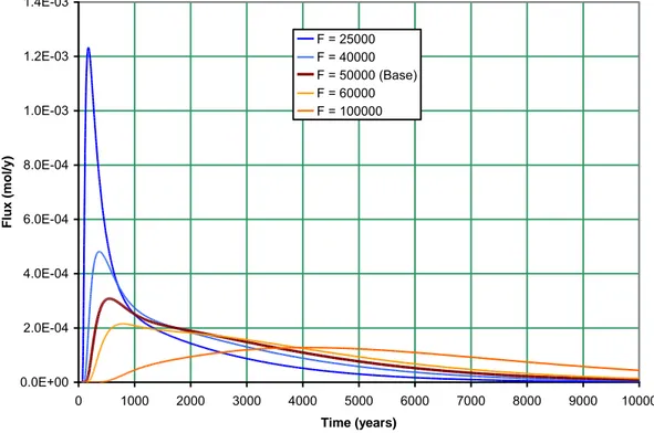
The F-factor characterises the degree of contact between the fracture and matrix. A higher F-factor corresponds to more contact and therefore to later and smaller peaks. We have run cases with a factor-of-two increase and decrease and with 20% increase and decrease. Figure 9 shows the results.
Figure 9: Sensitivity of flux output to varying F-factor for Se79 Case
0.0E+00 2.0E-04 4.0E-04 6.0E-04 8.0E-04 1.0E-03 1.2E-03 1.4E-03 0 1000 2000 3000 4000 5000 6000 7000 8000 9000 10000 Time (years) F lu x (mo l/ y) F = 25000 F = 40000 F = 50000 (Base) F = 60000 F = 100000
A factor-of-two reduction in F-factor leads to a factor-of-four increase in peak value for this case. The 20% reduction in F-factor changes the peak value by 60%, showing that this result is very sensitive to the F-value.
Travel time
The travel time corresponds to the time for water to pass through the system. In a case where matrix diffusion is significant, as it is here, the travel time itself is unlikely to be important, except through its indirect effect via the F-factor. We have run cases with a
factor-of-two increase and decrease and with 20% increase and decrease. Figure 10 shows the results.
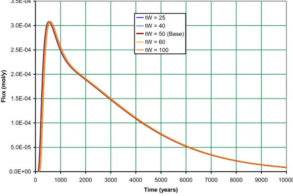
Figure 10: Sensitivity of flux output to varying Travel Time, tW, for Se79 Case
0.0E+00 5.0E-05 1.0E-04 1.5E-04 2.0E-04 2.5E-04 3.0E-04 3.5E-04 0 1000 2000 3000 4000 5000 6000 7000 8000 9000 10000 Time (years) F lu x (mo l/ y) tW = 25 tW = 40 tW = 50 (Base) tW = 60 tW = 100
As expected, varying the travel time has almost no effect if the F-factor is unchanged. For a case where matrix diffusion is unimportant, such as the I129 base case, the travel time would have a direct influence on the result.
Matrix penetration depth
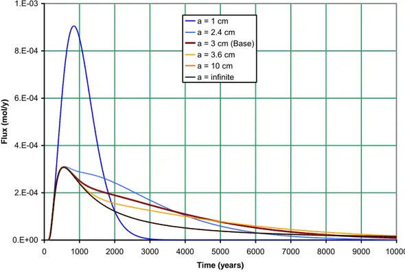
The matrix penetration depth controls the amount of sorptive capacity in the rock that is available. For small penetration depths this will directly control the flux, but for larger penetration depths it is the rate of diffusion into the matrix that controls the depth achieved and the result will tend towards a limit. We have run cases with a factor-of-three increase and decrease and with 20% increase and decrease. A case with infinite penetration depth was also run. Figure 11 shows the results.
Figure 11: Sensitivity of flux output to varying Maximum Penetration Depth, a, for Se79 Case 0.E+00 2.E-04 4.E-04 6.E-04 8.E-04 1.E-03 0 1000 2000 3000 4000 5000 6000 7000 8000 9000 10000 Time (years) F lu x (mo l/ y) a = 1 cm a = 2.4 cm a = 3 cm (Base) a = 3.6 cm a = 10 cm a = infinite
The infinite and 10 cm results are indistinguishable on this scale (they differ slightly at large times). In terms of the peak value, the result is the same for all the cases except the 1 cm case. This small penetration depth clearly allows for the rock matrix and fracture water to be in effective equilibrium, so that the overall effect is simply like that of retardation in the fracture.
Taking the formula given in (3.26), we can plot the extra average transport time (over the water travel time) as a function of the maximum penetration depth. This is shown in Figure 12, where the transition to the effectively infinite case can be seen to occur between 10 cm and 1 m. For depths less than around 20 cm the extra average transport time is linearly proportional to the maximum depth, but this measure does not provide information on the details of the peak response. The maximum extra travel time arises at a finite value of the depth because if the Se79 diffuses further than this then it decays before leaving the matrix and so does not contribute to the average travel time.
Figure 12: Extra Average Travel Time as a function of Maximum Penetration Depth, a, for Se79 Case
1.E+02 1.E+03 1.E+04 1.E+05
0.001 0.01 0.1 1 10 100
Maximum Penetration Depth (m)
Extr a T ravel T ime (y)
Matrix retention including porosity
Matrix retention and porosity always appear as a product in the solutions discussed earlier and represent a capacity of the matrix. The two uncertain parameters are the porosity itself and the Kd. For sorbed nuclides, the porosity component is negligible and the sorption dominates. The base case has a capacity factor of 2 (porosity 0.001, retention 2000). The capacity is expected to be important in directly controlling the amount of nuclide in the matrix compared to the fracture. We have run cases with a factor-of-two increase and decrease and with 20% increase and decrease. Figure 13 shows the results.
It is clear that the peak flux scales directly with the capacity factor in this range, due to the redistribution of material between stationary and flowing parts of the system.