Report number: 2009:17 ISSN: 2000-0456 Available at www.stralsakerhetsmyndigheten.se
Effect of Welding Residual Stresses
on Crack Opening Displacement and
Crack-Tip Parameters
Research
Authors:2009:17
Weilin Zang Jens Gunnars Jonathan Mullins Pingsha Dong Jeong K. HongTitle: Effect of Welding Residual Stresses on Crack Opening Displacement and Crack-Tip Parameters.
Report number: 2009:17
Authors: Weilin Zang 1), Jens Gunnars 1), Jonathan Mullins 1), Pingsha Dong2) and Jeong K. Hong2) 1)Inspecta Technology AB, Stockholm, Sweden. 2)Center for Welded Structures Research, Battelle,
Columbus, Ohio
Date: June 2009
This report concerns a study which has been conducted for the Swedish Radiation Safety Authority, SSM. The conclusions and viewpoints pre-sented in the report are those of the author/authors and do not neces-sarily coincide with those of the SSM.
Background
Weld residual stresses have a large influence on the behavior of cracks growing under normal operation loads and on the leakage-flow from a through-wall crack. Accurate prediction of these events is important in order to arrive at proper conclusions when assessing detected flaws, for inspection planning and for assessment of leak-before-break margins. The fracture mechanical treatment of weld residual stresses in common-ly used engineering assessment methods generalcommon-ly use the crack face pressure method and account neither for the displacement controlled nature of weld residual stresses, nor for multi-axial residual stresses. In this report, these effects are studied.
Objectives of the project
The principal objective of the project is to investigate the accuracy of the commonly used Crack Face Pressure (CFP) method, such as in the computer code ProSACC, for evaluating the stress intensity factor K for cracks located in multi-dimensional weld residual stress fields in piping geometries. Another aim is to investigate the accuracy of existing met-hods to evaluate the Crack Opening Displacement (COD) for through-wall cracks in pipes.
Results
The following conclusions can be made for cracks located in the vicinity of welds in piping geometries subjected to a combination of primary loads (during normal operation) and weld residual stresses:
• The CFP method gives a relatively good estimation of K for surface cracks.
• The CFP method cannot in general be demonstrated to give good accuracy for evaluating K for through-wall cracks even if good approximations exist for certain cases. The results in the report should be carefully studied for more guidance.
• The CFP method gives a relatively good estimation of the COD except for very long through-wall cracks.
• In the estimation of COD through the CFP method, plasticity ef-fects should be taken into account except for short through-wall cracks and low load levels.
Effects on SSM
The results of this project will be used by SSM in safety assessments of welded components with cracks and in assessments of Leak Before Break (LBB) applications.
Project information
Project leader at SSM: Björn Brickstad
Project number: 14.42-200542009, SSM 2008/77
Project Organisation: Inspecta Technology AB has managed the project with Dr Jens Gunnars as the project manager. Center for Welded Struc-tures Research, Battelle in Columbus, Ohio has been used as subcont-ractor to Inspecta Technology AB for certain project tasks.
1 (86)
Contents
1
SUMMARY...3
2
BACKGROUND ...4
3
OBJECTIVE ...6
3.1
Basis for crack-tip characterizing parameters ...6
3.2
Definition of leak before break parameters ...7
4
DEFINITION OF EVALUATED CALCULATION METHODS...9
4.1
Node relaxation in full 3D residual stress field (Control Method)...10
4.2
Elastic K results using weight functions (
oSACC Elastic KPr) ...10
4.3
Elastic FEM method (EL_b) ...10
4.4
COD using weight functions with plastic correction (NURBIT) ...10
4.5
Elastic-plastic FEM method (EP_b) ...11
4.6
FEM alternating method using infinite body solution (Alternating) ...11
5
DEFINITION OF CASE STUDIES...12
5.1
Pipe geometry, loading and material properties...12
5.2
Crack geometries...13
5.3
Weld geometry assumptions...13
6
CASE ONE - THIN PIPE WITH A THROUGH WALL CRACK ...14
6.1
Finite element models...14
6.2
2D welding simulation ...15
6.3
Crack profiles ...17
6.4
Maximum crack opening displacements ...21
6.5
Stress intensity factor...24
6.6
Crack tip opening displacements ...32
7
CASE TWO - THIN PIPE WITH A FULL CIRCUMFERENTIAL INTERNAL
SURFACE CRACK ...35
7.1
Finite element models...35
7.2
Crack profiles ...35
7.3
Stress intensity factor...38
7.4
Crack tip opening displacements ...41
8
CASE THREE - MEDIUM PIPE WITH A THROUGH WALL CRACK...42
8.1
Finite element model...42
8.2
Results from 2D welding simulation ...43
8.3
Crack profiles ...45
8.4
Maximum crack opening displacements ...49
8.5
Stress intensity factor...52
8.6
Crack tip opening displacements ...59
9
CASE FOUR - MEDIUM PIPE WITH A FULL CIRCUMFERENTIAL
INTERNAL SURFACE CRACK...61
9.1
Finite element model...61
9.2
Crack profiles ...61
9.3
Stress intensity factor...64
9.4
Crack tip opening displacements ...67
10
ALTERNATING FEM METHOD ...68
10.1
Residual Stress Mapping, 3D Model and Crack Definition...69
10.2
Results for Surface Cracks ...72
10.3
Results for Through-Wall Cracks ...76
10.4
Comparison to the crack face pressure method...80
11
DISCUSSION ...82
11.1
Crack opening displacements for leak before break assessments ...82
11.2
Crack-tip parameters for crack growth assessments ...82
11.3
COD for surface cracks and planning of visual inspection ...83
12
CONCLUSION ...84
13
FUTURE STUDIES ...85
3 (86)
1
SUMMARY
Weld residual stresses have a large influence on the behavior of cracks growing under normal operation loads and on the leakage-flow from a through-wall crack. The fracture mechanical treatment of weld residual stresses in commonly used engineering assessment methods generally use the crack face pressure method and account neither for the displacement controlled nature of weld residual stresses nor for multi-axial residual stresses. This work investigates the approximation of the crack face pressure method in the presence of weld residual stresses under normal operating conditions. Comparisons are made with a control method where the deformation controlled characteristics of weld residual stresses are considered.
For through wall cracks the crack opening area results are of interest for performing leak before break assessments. The main conclusion is that good agreement is obtained between the elastic-plastic FE method (crack face pressure method), NURBIT (crack face pressure method) and the control method for typical
minimum detectable crack sizes and load levels commonly seen in Swedish nuclear reactors (load level 1). The maximum observed variation between the methods was 26%, where COD was overestimated.
For full circumferential internal surface cracks K estimates are of interest for crack growth predictions. The main conclusions are:
For the 8 mm thick pipe there is generally good agreement between K predictions for the elastic ProSACC (crack face pressure) method and the control method for crack depths up to a/t=0.6. For the 32 mm thick pipe there is generally good agreement between K predictions for the elastic
ProSACC method and the control method. The largest variation of 15% was for the higher load level and deepest crack (a/t=0.8).
For the 32 mm thick pipe, where the axial weld residual stress profile is sinusoidal, the
surface COD due to ‘residual stresses only’ decreases rapidly, leading to the situation that it is
more difficult to detect
a deep crack than a shallow one. This may have implications for VT testing. For the 32 mm thick pipe, all methods predict crack arrest. For shallow cracks, K was overestimatedby all crack face pressure methods where there was a tensile residual stress near the inner wall.
2
BACKGROUND
Weld residual stresses have a large influence on the behavior of cracks growing under normal operation loads and on the leakage-flow from a through-wall crack. Accurate prediction of these events is important in order to arrive at proper conclusions when assessing detected flaws, for inspection planning or for assessment of leak-before-break margin.
A first prerequisite for performing these predictions is reliable prediction of the magnitude and distribution of welding residual stresses. This issue was addressed in a first stage of this project reported in [1], which had the purpose to validate and improve the weld residual stress modeling procedure used in Sweden [2].
The fracture mechanical treatment of weld residual stresses in commonly used engineering assessment methods generally account for neither the displacement controlled nature of weld residual stresses nor for multi-axial residual stresses. These issues are considered in this stage of the project.
Stress corrosion crack growth under normal operation loads
An important crack growth mechanism that has to be accounted for in performing inspection planning and structural integrity assessments of stainless steel components is stress corrosion cracking (SCC). For stress corrosion cracking to take place tensile stresses and an unfavourable environment are required. The mechanism is generally active under normal operation conditions. Since weld residual stresses usually are very high, they can have a significant influence on initiation and the subsequent growth of stress corrosion cracks. Crack growth rates are commonly expressed using the stress intensity factor K which characterizes the mechanical state at the crack-tip. Thus, the fracture mechanical treatment of weld residual stresses is of a great importance when predicting cracking of welded components.
Leak-before-break assessments
The leak-before-break (LBB) concept is sometimes applied for nuclear piping, in order to demonstrate that crack growth will result in a leak that is detectable, long before the crack reaches a critical size resulting in fracture. For example demonstration of LBB is sometimes applied in order to show that building of pipe break restraints is not necessary. LBB analyses may show that the margin against guillotine pipe break is very high, for a given leak detection capability, and hence pipe break restraints are unnecessary for reaching an acceptably low level of risk for dynamic events. In LBB analyses the weld residual stresses influence the conclusions about the leak-before-break margin, especially with respect to the estimated crack opening area (or crack opening displacement COD) and the corresponding leak rate.
Testing by visual inspection technique
One non-destructive inspection method that is increasingly used is the visual inspection technique (VT). In order to use the method cracks must be detectable for sizes that are smaller than the maximum allowable. In practice inspection at each location requires that residual stresses are present that open the crack mouth. To demonstrate that the postulated crack is detectable it is important to have an accurate prediction of the crack opening displacement (COD) at room temperature.
Determination of K and COD in residual stress fields
The stress intensity factor and crack opening displacement for a crack in a weld residual stress field can be determined in more than one way. For engineering assessments it is common to utilize a calculation procedure sometimes called the crack-face pressure method. By this method the stress in an uncracked model is extracted along the plane were the crack is postulated. Only the stress resolved normal to the crack plane is considered. This stress is applied to the crack surface in a model where the crack exists. This method is used both for direct calculation of K by FEM, and for derivation of weight functions by FEM or analytical methods.
5 (86)
The crack-face pressure method involves an assumption of load-controlled conditions, but is also valid for situations where remote displacements are applied. As long as the response is essentially linear, for example a large elastic specimen containing a short crack, and the loading is dominated by the normal stress component, the crack-face pressure method holds. However, for a crack growing in a weld, the assumptions of remote loading and linearity do not apply in general:
In a weld, the residual stress field is created by thermal and plastic strains generated in and around the weld metal. If the crack size is comparable to the radius of this region then the loading conditions should be treated as local and the remote loading assumption is no longer appropriate.
Significant plastic deformation may occur as the crack grows. The residual stress field must satisfy equilibrium conditions within the component of concern. For a growing crack, the residual stresses nearby re-distribute as stress-free surfaces are generated, while for load-controlled conditions the far-field stresses can be assumed to be stationary.
Weld residual stress fields are triaxial so in these cases it cannot be assumed that loading is dominated by the normal stress component.
In spite of these limitations the crack-face pressure method is widely used. Thus it is important to investigate under which conditions the method remains conservative for calculation of the stress intensity factors and crack openings.
3
OBJECTIVE
This work investigates the treatment of weld residual stresses when performing fracture mechanical analysis of welded components. The objective is to determine if it is conservative to use the crack face pressure method for crack shapes and loading cases that might be found under normal operating conditions. The magnitude of the residual stress field and crack characterizing parameters affects crack growth and leak-before-break predictions in different ways, and accurate and conservative estimates are important.
Detailed simulations are made where a crack is created in full 3D weld residual stress fields by use of the node-relaxation technique. The crack-tip characterizing parameters and the crack opening displacement determined from this model are compared with results obtained from different implementations of the crack face pressure method. Of particular interest is comparison and validation of the prediction of the ProSACC stress corrosion crack growth module and NURBIT. Two pipe geometries with surface and through wall cracks are studied for normal operation cases where the weld residual stresses constitute a significant part of the loading. Also the alternating method is considered.
3.1
Basis for crack-tip characterizing parameters
In this investigation crack growth under normal operation is of interest. Relations that describe crack growth due to fatigue or stress corrosion normally use the elastic stress intensity factor K as the parameter describing the mechanical state at the crack tip. Values for K can be directly extracted from finite element models through nodal extrapolation from the near-tip finite element mesh. This method, however, requires a very fine mesh which makes analysis computationally expensive, especially in 3D models such as those considered in this study. Further, K is an elastic crack tip parameter and the test cases considered in this study involve ductile materials for which considerable plastic deformation may occur around the crack tip. For these reasons, the natural alternative crack tip parameter to consider is the J-integral. It can be shown to characterize the stresses and strains near the crack-tip in elastic-plastic materials and is also an energy conservation integral.
The standard J-integral is known to be unique for plastic materials provided unloading does not occur. However, it is path dependent for a growing crack in an elastic-plastic material (due to unloading in the wake) and also in the presence of a weld residual stress field. This has spawned considerable efforts in recent years to develop a path-independent form of J [3-6], where the influence of prior plastic deformation is decoupled from the standard surface integral and included as an additional term in the formulation. These efforts were
successful and the modified J-integral formulation shows path-independence under combinations of residual stress and mechanical loading. Further, the modified J is also shown to be equivalent to the stress intensity factor K in cases of small scale yielding. The calculated J in this investigation will be converted to an equivalent stress intensity factor using the relation,
K
J
E
/(
1
2)
(3.1)where E is Young’s modulus and is Poisson’s ratio.
Studies on the modified J-integral [4-7] have also demonstrated that the standard J-integral can be used to provide an accurate estimate, provided that the evaluation path is suitably near to the crack tip. It has been found that in an area very close to the crack tip, J evaluated by the standard definition and by the modified definition both result in an almost identical value [4]. The reason for this is that the contribution from the additional ‘prior plastic deformation’ term vanishes to zero when the integral is evaluated very close to the crack tip [4]. One conclusion from this is that by using the modified
7 (86)
In [4-7] the difference between the standard and the modified J-integral tends to decrease as the primary load decreases. In this investigation we are focusing on growth and leakage under normal operation loads, and not on the prediction of fracture due to high primary loads. In order to conclude on the distance at which the two integrals become identical, it is necessary to calculate both the standard and the modified integral for the present loading situation. In the present investigation an implementation of the modified J-integral was not available for 3D cases so, alternatively, near-tip estimates of the standard J-integral are used. It is judged that the standard J-integral evaluated close enough to the crack-tip is sufficient to demonstrate the key trends for the present investigation. The standard J-integral evaluated between 0.01 and 0.1 mm from the crack tip is used. An alternative measure for the near-tip state is CTOD [8]. The definition is illustrated in Figure 3.1. For an
elastic-plastic material when no unloading occurs CTOD has a simple relation with the standard
J-integral [8].
Figure 3.1 Definition of CTOD.
While CTOD could provide a valid measure of the mechanical state at the crack tip, the crack growth relations are usually based upon K, and it is more difficult to convert CTOD to K. It is typically more convenient to use the J-integral and equivalent K, although CTOD values are reported here.
3.2
Definition of leak before break parameters
The crack opening area COA is a key parameter for estimation of leakage rates in leak-before-break assessments. In the current investigation we will study the parameters defined below.
Figure 3.2 shows a through wall crack of length 2a approximated by an elliptical function. For such a geometry the crack opening displacement can be expressed as
2/
1
l
a
u
e
, (3.2)where
e is the the crack opening displacement at the mid point of the crack. Integrating the displacement results in the (elastic) crack opening areaa COAe
e2
. (3.3)
Figure 3.2 Elliptical model for crack opening displacement (through wall case).
The COA for each method can be compared directly. As seen above it is also possible to compare an equivalent maximum crack opening displacement, which will accentuate the difference in the crack opening area
calculated by the different methods. We will present the results as an equivalent crack opening parameter defined by
* * 2 a COA , (3.4)9 (86)
4
DEFINITION OF EVALUATED CALCULATION METHODS
The different analysis methods evaluated for treatment of weld residual stresses are summarized in the table below.
Table 4.1. Notation and overview of the compared calculation methods. Method
denotation
Short description of calculation method Parameters
evaluated Control FEM, near tip J-integral calculation
Node relaxation of crack Full 3D residual stress field Elastic-plastic model
Considered as the most accurate simulation method.
K, CTOD
COD,
oSACC Elastic
KPr Weight functions, solutions determined for load controlled boundary conditions using the crack face pressure method Normal stresses taken from uncracked body
Elastic model
K
EL_b FEM, near tip J-integral calculation Crack face pressure
Normal stresses taken from uncracked body Elastic model
K, CTOD
COD,
NURBIT Weight functions, solutions determined for load controlled boundary conditions using the crack face pressure method Normal stresses taken from uncracked body
Elastic model using plastic correction
EP_b FEM, near tip J-integral calculation Crack face pressure
Normal stresses taken from uncracked body Elastic plastic model
K, CTOD
COD,
Alternating FEM alternating method (coupled, iterative FE/analytical method)
Infinite body KI solution Elastic
Full 3D residual stress field applied
K
COD,
4.1
Node relaxation in full 3D residual stress field (Control Method)
This simulation method is designed to best simulate the growth of a crack in a residual stress field. The procedure is as follows:
A 2D axi-symmetrical welding simulation is performed. The new welding simulation procedure according to [1] is applied.
Hydro-test pressure is applied and released at 20 °C.
The 2D solution is mapped into a 3D model with a crack. At this stage nodes along the crack are constrained. The operating loads (membrane stress plus bending stress) are applied (load case 1).
Crack growth is activated by instantaneously releasing the constraints on the crack face nodes.
J-integrals, COD and CTOD are calculated.
Finally the primary loads are increased to a slightly higher level, called load case 2. The J-integral, COD and CTOD are calculated for this load case.
The results generated in this manner are considered as the most accurate results.
4.2
Elastic K results using weight functions (
oSACC Elastic KPr)
This method uses the crack face pressure assumption. Elastic weight functions are used to calculate K values due to primary and secondary loads. These results are useful for assessment of crack growth calculations.
4.3
Elastic FEM method (EL_b)
This method uses the crack face pressure assumption where the stress in an uncracked model is extracted along the plane where the crack is postulated. Only the stress resolved normal to the crack plane is considered. This stress is applied to the crack surface in a model where the crack exists.
This method uses linear elastic finite element calculation and the residual stress obtained from the 2D welding simulation is applied as the crack face pressure.
The J-integral, COD and CTOD are calculated for two load cases. Results are denoted EL_b. Results for the residual stress only are denoted EL (Resi. only). This model is very similar to the KElasticProSACC
model
4.4
COD using weight functions with plastic correction (NURBIT)
The calculation procedures are similar to those used in ProSACC with the exception that some solutions are more detailed with regards to through wall crack geometries. In contrast to ProSACC, estimates of COD (and COA) can be extracted from NURBIT [10]. A plastic correction is also applied and details are available in [10].
11 (86)
4.5
Elastic-plastic FEM method (EP_b)
The calculation procedure is identical with the elastic FEM method, with the exception that the material response is elastic-plastic.
The J-integral, COD and CTOD are calculated for two load cases. Results are denoted by EP_b. Elastic-plastic FEM analyses of cracks using the crack face pressure method are most relevant for COD
assessment of fracture but not for crack growth assessments.
4.6
FEM alternating method using infinite body solution (Alternating)
The method involves an iterative procedure using a coupled finite element and infinite body (analytical)
solution [11, 12]. This method uses an elastic constitutive model. A full 3D residual stress field is applied as an initial condition in an uncracked FE model. The FEM boundary conditions are successively updated until they display a (nearly) stress free state along the postulated crack surface. At the same time the crack face pressure in an infinite body crack model is successively updated until it converges. The alternating method is described in detail in chapter 10.
5
DEFINITION OF CASE STUDIES
The different analysis methods will be evaluated for four cases which represent loading scenarios that occur under normal operation of a nuclear power plant. The four cases were taken from a LBB study [13]. A thin and a medium thickness pipe are chosen, containing first a through wall crack and then an internal surface crack. Four crack sizes are considered for each crack geometry. As discussed in this chapter, two load levels are specified – in an effort to cover the range of conditions experienced under normal operation.
5.1
Pipe geometry, loading and material properties
A thin pipe and a medium pipe are selected for investigation. The geometries and mechanical loadings for the chosen cases are shown in Table 5.1 and 5.2. Note that in Table 5.2 the axial membrane stress is entirely due to internal pressure. The load case L2 deviates from [13] and is introduced to represent slightly higher loads than normal; in this case the bending load specified in load case L1 was doubled. The pipes are made of stainless steel TP304. The material properties used in the analysis are listed in Table 5.3. Bilinear isotropic hardening was specified.
Table 5.1 Geometry.
Inner pipe radius (mm)
Thickness, t (mm)
Thin pipe 153.6 8.3
Medium pipe 146 31.8
Table 5.2 Applied mechanical loads for load levels 1 and 2.
Load Level 1 (L1) Load level 2 (L2)
Temperature (°C) Internal pressure (MPa) Axial membrane stress (MPa) Bending stress (MPa) Axial membrane stress (MPa) Bending stress (MPa) Thin pipe 145 4.6 41 32 41 64 Medium pipe 323 15.5 32.1 19 32.1 38
Table 5.3 Material properties
Temperature (°C) TP304 Weld material 100 195 195 200 185 185 E (GPa) 400 170 170
0.3 0.3 100 173 419 200 140 368 y
(MPa) 400 116 26413 (86)
5.2
Crack geometries
Cracks growing along the weld centerline are studied. Two crack geometries are considered:
A through wall circumferential crack. Four different crack lengths are evaluated, specified as shown in Table 5.4.
A complete circumferential internal crack. Four different crack depths a are considered,
a/t = 0.2, 0.4, 0.6 and 0.8.
In the LBB study [13] the crack size was determined for a leakage rate of 10 gallons per minute. In reality this crack size is heavily dependent on the crack face morphology and for this reason different crack sizes were specified in Table 5.4, corresponding to typical observed morphologies.
The detectable through wall crack sizes considered are listed in Table 5.4. The maximum allowable crack size was also considered, although the shorter crack sizes are of greater interest because weld residual stresses make a larger contribution to the loading. A further reason why the shorter cracks are of more interest is that a crack spends most of its lifetime in stable growth, not at the maximum allowable size.
Table 5.4 Detectable through wall crack sizes chosen for evaluation [13].
Thin pipe
(mm)
Medium pipe
(mm)
Comments
137
175
Crack size resulting in detectable leakage (load
level 1). Assumed crack morphology, ‘fatigue 1.’
160
218
Crack size resulting in detectable leakage (load
level 1). Assumed crack morphology, ‘fatigue 2.’
185
246
Crack size resulting in detectable leakage (load
level 1). Assumed crack morphology, ‘PWSCC.’
350
330
Maximum allowable crack size, [13].
5.3
Weld geometry assumptions
Four weld passes are used for the thin walled pipe and twelve weld passes for the medium thickness pipe. The heat input is defined according to the phase 1 report from this project [1]. Welding is simulated using
6
CASE ONE - THIN PIPE WITH A THROUGH WALL CRACK
6.1
Finite element models
The finite element mesh used for 2D welding simulation and the weld pass order is shown in Figure 6.1. The finite element mesh for the 3D fracture mechanics model with a through wall crack is shown in Figure 6.2. A small notch with a notch radius of 0.001 mm is introduced at the crack tip – this allows an accurate prediction of near-tip-J and CTOD.
Figure 6.1 Finite element mesh for 2D welding simulation for case 1.
l
Figure 6.2 Case 1 - finite element mesh with a through thickness crack. The coordinate l = 0 corresponds to the center of the through wall crack, as previously defined in Figure 3.2.
15 (86)
6.2
2D welding simulation
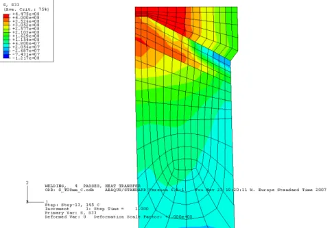
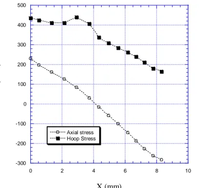
The welding residual stress distribution at the operating temperature is shown in Figures 6.3 and 6.4. The axial residual stress along the weld centre is a bending stress, as illustrated in Figure 6.5
Figure 6.3 Welding residual stress in the axial direction at the operating temperature.
-300 -200 -100 0 100 200 300 400 500 0 2 4 6 8 10 Axial stress Hoop Stress X (mm)
Figure 6.5 Welding residual stresses along the weld centre line. X is measured through the thickness from the pipe’s inner surface.
17 (86)
6.3
Crack profiles
Crack profiles determined by the different evaluation methods are shown in Figures 6.6-6.9 for the four different through wall crack lengths. Results are shown for the two load levels L1 and L2. In the figures, open symbols indicate results at load level 1 and the solid symbols for load level 2. The figures are split into two parts: a) gives crack opening displacement COD results for the pipe inner surface and b) for the pipe outer surface. Results due to residual stress only calculated by the elastic FEM method are also included.
When compared with the control method, it is observed that the COD calculated by the elastic FEM method (EL_b) is underestimated, and the COD calculated by the elastic-plastic FEM method (EP_b) is overestimated. If the results are used for an LBB-analysis or assessment of detection by visual inspection technique, the results from the elastic FEM method are conservative in the sense that they under-predict the leak rate and the crack opening. The results from the elastic-plastic FEM method are non-conservative in the same sense.
Note that for one of the analysed cases the crack profile predicted by the elastic FEM method (EL_b) and the control method coincide, as indicated in Figure 6.6b. This could be explained by an essentially elastic behavior for this low load level and short crack. As the crack length is increased by 17%, we start to see a discrepancy, see Figure 6.7b. 0 0,1 0,2 0,3 0,4 0,5 0 10 20 30 40 50 60 70 Control (L1) EL_b (L1) EP_b (L1) EL (Resi. Only) Control (L2) EL_b (L2) EP_b (L2) l (mm)
Figure 6.6a COD along pipe inner surface for crack length 137 mm. L1 indicates the results at load level 1 and L2 at the higher load level 2. See Table 4.1 for the notation of the methods.
-0,1 0 0,1 0,2 0,3 0,4 0,5 0 10 20 30 40 50 60 70 Control (L1) EL_b (L1) EP_b (L1) EL (Resi. Only) Control (L2) EL_b (L2) EP_b (L2) l (mm)
Figure 6.6b COD along pipe outside surface for crack length 137 mm
0 0,1 0,2 0,3 0,4 0,5 0 10 20 30 40 50 60 70 80 Control (L1) EL_b (L1) EP_b (L1) EL (Resi only) Control (L2) EL_b (L2) EP_b (L2) l (mm)
19 (86) -0,2 -0,1 0 0,1 0,2 0,3 0,4 0,5 0 10 20 30 40 50 60 70 80 Control (L1) EL_b (L1) EP_b (L1) EL (Resi. Only) Control (L2) EL_b (L2) EP_b (L2) l (mm)
Figure 6.7b COD along pipe outer surface for crack length 160 mm.
0 0,1 0,2 0,3 0,4 0,5 0,6 0,7 0,8 0 20 40 60 80 100 Control (L1) EL_b (L1) EP_b (L1) EL (Resi. only) Control (L2) EL_b (L2) EP_b (L2) l (mm)
-0,2 0 0,2 0,4 0,6 0,8 0 20 40 60 80 100 Control (L1) EL_b (L1) EP_b (L1) EL (Resi. only) Control (L2) EL_b (L2) EP_b (L2) l (mm)
Figure 6.8b COD along pipe outer surface for crack length 185 mm.
0 1 2 3 4 5 6 7 8 0 50 100 150 200 Control (L1) EL_b (L1) EP_b (L1) EL (Resi. only) Control (L2) EL_b (L2) EP_b (L2) l (mm)
21 (86) 0 2 4 6 8 10 0 50 100 150 200 Control (L1) EL_b (L1) EP_b (L1) EL (Resi. only) Control (L2) EL_b (L2) EP_b (L2) l (mm)
Figure 6.9b COD at pipe outer surface for crack length 350 mm.
6.4
Maximum crack opening displacements
As discussed in section 3.2 the integrated crack opening area may be represented by an equivalent crack
opening parameter, Predictions from the FE analyses (from the previous section) are presented in Tables 6.1-6.2 and in Figure 6.10. Predictions from NURBIT are also shown.
When compared with the control method, it is observed that the calculated by the elastic-plastic FEM method (EP_b) is slightly overestimated for the shorter cracks (corresponding to the detectable sizes from Table 5.1). The
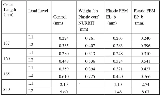
calculated by NURBIT is similar to the results by EP_b. For the crack lengths up to 185 mm, the crack opening area is overestimated by 7-26% for the lower load case L1. Comparison to calculated by the elastic FEM method indicates that plastic effects are substantial even for the moderate crack lengths and low load level.Table 6.1 Equivalent crack opening parameter
at pipe inner surface. Crack Length (mm) Load Level Control (mm) Weight fcn Plastic corrn NURBIT (mm) Elastic FEM EL_b (mm) Plastic FEM EP_b (mm) L1 0.224 0.261 0.205 0.240 137 L2 0.335 0.407 0.263 0.396 L1 0.280 0.313 0.248 0.310 160 L2 0.448 0.536 0.324 0.541 L1 0.359 0.394 0.321 0.427 185 L2 0.610 0.725 0.420 0.766 L1 2.10 - 1.10 2.74 350 L2 5.60 - 1.48 8.07Table 6.2 Equivalent crack opening parameter
at pipe outer surface. Crack Length (mm) Load Level Control (mm) Weight fcn Plastic corrn NURBIT (mm) Elastic FEM EL_b (mm) Plastic FEM EP_b (mm) L1 0.081 0.070 0.083 0.123 137 L2 0.209 0.268 0.156 0.316 L1 0.140 0.127 0.128 0.199 160 L2 0.335 0.414 0.221 0.475 L1 0.223 0.218 0.207 0.328 185 L2 0.511 0.633 0.325 0.720 L1 2.06 - 1.00 2.74 350 L2 5.79 - 1.41 8.4023 (86) 0 0,2 0,4 0,6 0,8 1 100 120 140 160 180 200 Control (L1) EL_b (L1) EP_b (L1) NURBIT (L1) Control (L2) EL_b (L2) EP_b (L2) NURBIT (L2) Crack Length (mm)
Figure 6.10a. Equivalent crack opening parameter at inside surface of pipe. In the figure L1 indicates the results at load level 1 and L2 at load level 2.
0 0,3 0,6 0,9 1,2 1,5 100 120 140 160 180 200 Control (L1) EL_b (L1) EP_b (L1) NURBIT (L1) Control (L2) EL_b (L2) EP_b (L2) NURBIT (L2) Crack Length (mm)
Figure 6.10b. Equivalent crack opening parameter at outside surface of pipe.
6.5
Stress intensity factor
The stress intensity factor calculated in this section is based on the near-tip J-integral. Eq. (3.1) is used to obtain
K. The standard J-integral, when evaluated close enough to the crack-tip will provide an accurate estimate of
the J-integral calculated using the integral modified to account for residual stresses, as discussed in Section 3.1. The J-integral along different paths is shown in Figure 6.12 for the case of a 160 mm long crack. The crack is
simulated using the control method. Figure 6.12a demonstrates that the standard integral is, in general, path dependent. However, close enough to the crack tip, path independence is displayed as proposed in [4]. In this case, within 1 mm from the crack tip the J-integrals are almost path independent. Figure 6.12b shows a detailed view of the paths very close to the crack-tip. The J-integral is evaluated for three different positions along the crack front as defined in Figure 6.11.
1 3 2 1 1 3 2 1
Figure 6.11. Definition of evaluation points along the crack front of the through wall crack. Crack locations 1, 2 and 3 are also refered to as Loc 1, Loc 2 and Loc 3.
For this case it was chosen to determine K based on J-integrals calculated at 0.1 mm from the crack-tip (path 10 from the tip).
25 (86) -40 -20 0 20 40 0 1 2 3 4 5 Loc 1 (Load 1) Loc 2 (Load 1) Loc 3 (Load 1) Loc 1 (Load 2) Loc 2 (Load 2) Loc 3 (Load 2) r (mm)
Figure 6.12a. J-integrals as function of distance r from the crack-tip for a crack simulated by the control method (crack length 160 mm).
-10 0 10 20 30 40 50 0 0,1 0,2 0,3 0,4 0,5 Loc 1 (Load 1) Loc 2 (Load 1) Loc 3 (Load 1) Loc 1 (Load 2) Loc 2 (Load 2) Loc 3 (Load 2) r (mm)
Figure 6.12b. J-integrals as function of distance r from the crack-tip for a crack simulated by the control method (crack length 160 mm). The 25 near-tip paths are shown.
The distributions of stress intensity factors along the crack front are shown in Figures 6.13-6.15. Results for three different methods are presented: control, elastic FEM and plastic FEM.
The most relevant comparison for crack growth assessments is the difference between the control method and the elastic FE method, because the growth calculations in ProSACC are made using linear elastic solutions. For the moderate cracks up to 185 mm the results for EL_b and control agree well, except at the pipe inside.
Below is a discussion about the deviation in K that is observed for the control method near the inner surface of the pipe. As discussed in the background, the different evaluation methods are based on different modeling assumptions. For example, the high out-of-plane residual stress is only included in the control method. Below some efforts are made to understand the important assumptions in the different models. Note that for the control method K actually decreases approaching the pipe inner surface. Such a results has not previously been observed by the authors and requires further investigation.
We first consider the results for the largest crack (a=350 mm) and the highest loading (L2). In this case the contribution from the residual stress is minimal as seen in Figure 6.15. This allows a comparison of the control method and the elastic-plastic FE method for a case dominated by primary loading. It is seen that the K-values predicted by the control method are consistently lower than those predicted by the elastic-plastic FE method. Since the contribution from the residual stresses to K is small, the major difference between these methods is that a high out-of-plane stress is only applied in the case of the control method (see the hoop stress from Figure 6.5). Addition of such an out-of-plane stress will increase the hydrostatic stress component and suppress near-tip plasticity which might explain the consistently lower reported K value, where K was converted from J using equation 3.1.
Considering then the other crack sizes and load levels, a somewhat different trend emerges. Towards the outer edge of the pipe the results for the elastic-plastic FE and control methods are in reasonably good agreement. The larger difference in predictions is seen towards the inner pipe surface. In this region the residual stresses are tensile and constitute a large proportion of the loading. At the outside the residual stress is compressive. It is hard to differentiate whether the difference towards the inner surface is due to the out-of-plane stress or due to the displacement controlled nature of the residual stress modelled by the control method.
Comparing the elastic FE and elastic-plastic FE models two observations can be made. For low loads the two methods are nearly identical. For high loads, and the largest crack size, higher K-predictions are obtained for the elastic-plastic FE method than for the elastic FE method. These trends may be explained by increased crack tip plasticity in the elastic-plastic FE model for increases in load and crack size. Increased crack tip plasticity effectively increases the crack size and therefore also increases the estimated value of K.
A final observation regarding the Figures 6.13 to 6.15 regards application of the different evaluation methods for crack growth calculations. Compared to the control method, the K-value calculated by the elastic-plastic FE method is conservative, whereas the elastic FE method is non-conservative.
27 (86) -50 0 50 100 150 0 0,2 0,4 0,6 0,8 1 Control (L1) EL_b (L1) EP_b (L1) EL (Resi. only) Control (L2) EL_b (L2) EP_b (L2) x/t
Figure 6.13 Stress intensity factors along the crack front for crack length 160 mm. In the figure, x = 0 at the pipe inner surface, L1 indicates the results at load level 1 and L2 at load level 2.
-50 0 50 100 150 0 0,2 0,4 0,6 0,8 1 Control (L1) EL_b (L1) EP_b (L1) EL (Resi. only) Control (L2) EL_b (L2) EP_b (L2) x/t
Figure 6.14 Stress intensity factors along the crack front for crack length 185 mm. In the figure, x = 0 at the pipe inner surface, L1 indicates the results at load level 1 and L2 at load level 2.
-100 0 100 200 300 400 500 0 0,2 0,4 0,6 0,8 1 Control (L1) EL_b (L1) EP_b (L1) EL (Resi. only) Control (L2) EL_b (L2) EP_b (L2) x/t
Figure 6.15 Stress intensity factors along the crack front for crack length 350 mm. In the figure, x = 0 at the pipe inner surface, L1 indicates the results at load level 1 and L2 at load level 2.
The results are also shown in Tables 6.5-6.6. Results from the software package ProSACC are included for comparison. For crack growth calculations it may be concluded that the elastic ProSACC predictions overestimate K near the inner surface of the pipe, in comparison to the control results.
Note that the maximum value of K is not always obtained at the inner or outer surfaces for the control method and EP_b, see Figure 6.15. This could have implications for predictions using ProSACC since only values at the surfaces are provided from ProSACC.
29 (86)
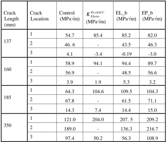
Table 6.5 Stress intensity factors estimated using different methods at load level 1.
Crack Length (mm) Crack Location Control (MPa√m) oSACC Elastic KPr (MPa√m) EL_b (MPa√m) EP_b (MPa√m) 1 54.7 85.4 85.2 82.0 2 46. 6 - 43.5 46.3 137 3 4.1 -3.4 -0.19 -3.0 1 58.9 94.1 94.4 89.7 2 56.9 - 48.5 56.6 160 3 3.9 1.9 5.3 3.2 1 64.3 104.6 109.5 104.3 2 67.8 - 61.5 71.1 185 3 14.3 7.4 14.4 15.0 1 121.0 204.0 207. 5 209.2 2 189.0 - 136.3 216.7 350 3 97.4 50.2 56.3 108.9
Table 6.6 Stress intensity factors estimated using different methods at load level 2.
Crack Length (mm) Crack Location Control (MPa√m) oSACC Elastic KPr (MPa√m) EL_b (MPa√m) EP_b (MPa√m) 1 67.4 105.2 103.8 106.4 2 72.0 - 60. 7 76.1 137 3 24.5 16.8 18.0 20.3 1 75.2 117.8 116.5 118.0 2 88.8 - 72.0 92.0 160 3 37.1 24.1 25.5 30. 5 1 84.0 132.9 135.9 137.9 2 106.1 - 86.7 112.8 185 3 48.8 31.8 36.5 47.5 1 228.3 270.5 308.0 333.7 2 365.2 - 183.2 442.5 350 3 187.5 88.2 51.7 237.5 SSM 2009:17
Tables 6.7 and 6.8 are included to show the contribution from the residual stress to K for the load cases chosen for analysis in this investigation. The contribution at the inner surface is about 50% for the shortest crack and the low primary loading L1.
Table 6.7 Comparison showing the contribution of the residual stress to K calculated using the elastic-plastic FE method (load level L1).
Crack Length (mm) Crack Location Without residual stresses, (MPa√m) With residual stresses, (MPa√m) 1 44.9 82.0 2 54.7 65.0 137 3 43.7 -3.0 1 53.0 89.7 2 64.9 75.6 160 3 50.3 3.18 1 64.1 104.3 2 77.4 84.4 185 3 58.6 15.0 1 173.7 209.1 2 222.9 234.7 350 3 156.9 108.9
31 (86)
Table 6.8 Comparison showing the contribution of the residual stress to K calculated using the elastic-plastic FE method (load level L2).
Crack Length (mm) Crack Location Without residual stresses, (MPa√m) With residual stresses, (MPa√m) 1 69.4 106.4 2 84.8 95.1 137 3 67.0 20.3 1 81.3 118.0 2 100.6 111.4 160 3 77.5 30. 5 1 97.7 137.9 2 120.7 127.8 185 3 91.1 47.5 1 298.3 333.7 2 460.7 472.5 350 3 285.5 237.5 SSM 2009:17
6.6
Crack tip opening displacements
Crack tip opening displacements were calculated at the three locations indicated in Figure 6.11. The results are listed in Tables 6.9-6.10 and are also plotted in Figure 6.17a and b to allow better visualization. These results show that the elastic FE method underestimates CTOD. For the three largest crack lengths the elastic-plastic FE method overestimates CTOD.
Table 6.9 Crack tip opening displacements estimated using different methods load level 1. Crack
Length
(mm) Crack Location Control (mm)
Elastic FEM EL_b (mm) Elastic-plastic FEM EP_b (mm) 1 0.0095 0.0018 0.0080 2 0.0088 0.0009 0.0113 137 3 -0.0004 0.0000 0.0053 1 0.0115 0.0017 0.0112 2 0.0125 0.0018 0.0164 160 3 -0.0001 0.0015 0.0074 1 0.0142 0.0023 0.0167 2 0.0175 0.0014 0.0240 185 3 0.0004 0.0003 0.0108 1 0.0924 0.0029 0.1053 2 0.1332 0.0029 0.1857 350 3 0.0361 0.0011 0.3488
33 (86)
Table 6.10 Crack tip opening displacements estimated using different methods load level 2. Crack
Length
(mm) Crack Location Control (mm)
Elastic FEM EL_b (mm) Elastic-plastic FEM EP_b (mm) 1 0.0156 0.0022 0.0201 2 0.0200 0.0013 0.0296 137 3 0.0015 0.0004 0.0149 1 0.0210 0.0024 0.0287 2 0.0294 0.0016 0.0420 160 3 0.0038 0.0005 0.0213 1 0.0281 0.0029 0.0456 2 0.0425 0.0019 0.0600 185 3 0.0068 0.0008 0.0326 1 0.1774 0.0042 0.3289 2 0.4379 0.0025 0.7011 350 3 0.1338 0.0019 0.2936 SSM 2009:17
-0,008 0 0,008 0,016 0,024 100 120 140 160 180 200 Control (Loc 1) EL_b (Loc 1) EP_b (Loc 1) Control (Loc 2) EL_b (Loc 2) EP_b (Loc 2) Control (Loc 3) EL_b (Loc 3) EP_B (Loc 3) Crack Length (mm)
Figure 6.17a. Crack tip opening displacements for load level 1.
0 0,012 0,024 0,036 0,048 0,06 100 120 140 160 180 200 Control (Loc 1) EL_b (Loc 1) EP_b (Loc 1) Control (Loc 2) EL_b (Loc 2) EP_b (Loc 2) Control (Loc 3) EL_b (Loc 3) EP_B (Loc 3) Crack Length (mm)
35 (86)
7
CASE TWO - THIN PIPE WITH A FULL CIRCUMFERENTIAL INTERNAL
SURFACE CRACK
7.1
Finite element models
The pipe geometry considered in case two is the same as for case one with the difference that a full
circumferential, internal surface crack is modeled, as opposed to a through-wall crack. The finite element mesh used for welding simulation is also the same, as shown in Figure 7.1. The finite element mesh for the fracture mechanics model is, however, different. A 2D, axisymmetric model was used and is illustrated in Figure 7.1. The notch radius is 0.001mm, allowing accurate prediction of near-tip-J and CTOD.
Figure 7.1 Case 2 – 2D axisymmetric finite element mesh for the full circumferential, internal surface crack.
7.2
Crack profiles
Crack profiles through the thickness are shown in Figures 7.2 to 7.5 for the different evaluation methods. Each figure represents a different crack depth, ranging from a/t=0.2 to 0.8. Results are shown for the two load levels L1 and L2. In the figures, open symbols indicate results at load level 1 and the solid symbols at load level 2. Results due to residual stresses only, calculated by the elastic FE method, are also included.
Note that the crack opening displacement due to welding residual stress contributes approximately 50% of the total COD for both the elastic and elastic-plastic FE methods. Inclusion of weld residual stresses is therefore very important in computation of COD for these cases.
It is observed that the crack opening displacement predicted by the elastic FE method and the elastic-plastic FE method are nearly identical when a/t < 0.6. This implies that the effect of plastic deformation in these cases is very limited. In comparison to the control method, both the elastic and elastic-plastic FE methods
underestimate the crack opening displacement for a/t up to 0.6. For a/t equal to 0.8, the same trend is again observed for the lower load level L1, but for the higher load level L2, the COD for the elastic-plastic FE method is overestimated. The difference between the control method and EP_b could be due to the displacement controlled model and the high out-of-plane stress.
Note that for conclusions on VT inspection results for the control method and residual stresses only would be needed, since VT is performed in a state without pressure.
x
0 3 6 9 12 0 0,5 1 1,5 2 Control (L1) EL_b (L1) EP_b (L1) EL (Resi. only) Control (L2) EL_b (L2) EP_b (L2) x (mm)
Figure 7.2 COD for crack depth a/t = 0.2. x = 0 at the pipe inner surface.
0 6,25 12,5 18,75 25 0 1 2 3 4 Control (L1) EL_b (L1) EP_b (L1) EL (Resi. only) Control (L2) EL_b (L2) EP_b (L2) x (mm)
Figure 7.3 COD for crack depth a/t = 0.4. x = 0 at the pipe inner surface.
COD (m)
37 (86) 0 10 20 30 40 50 60 70 0 1 2 3 4 5 Control (L1) EL_b (L1) EP_b (L1) EL (Resi. only) Control (L2) EL_b (L2) EP_b (L2) x (mm)
Figure 7.4 COD for crack depth a/t = 0.6. x = 0 at the pipe inner surface.
0 40 80 120 160 0 2 4 6 8 Control (L1) EL_b (L1) EP_b (L1) EL (Resi. only) Control (L2) EL_b (L2) EP_b (L2) x (mm)
Figure 7.5 COD for crack depth a/t = 0.8. x = 0 at the pipe inner surface.
COD (m)
COD (m)
7.3
Stress intensity factor
As in Section 6.5 the stress intensity factor calculated in this section is based on the near-tip J-integral. Eq. (2.1) is used to obtain K. The J-integrals for crack depth a/t = 0.6 are shown in Figure 7.6. It is shown that the
J-integrals are strongly path dependent about 0.05 mm away from crack tip. Within 0.05 mm from the crack tip, J-integrals are almost path independent.
12 14 16 18 20 22 24 0 0,1 0,2 0,3 0,4 0,5 J (Meth 1 Load 1) J (Meth 1 Load 2) x (mm)
Figure 7.6a. J-integrals by Control Method for crack depth a/t = 0.6 (including remote paths).
12 14 16 18 20 22 24 0 0,01 0,02 0,03 0,04 0,05 J (Meth 1 Load 1) J (Meth 1 Load 2) x (mm)
Figure 7.6b. J-integrals by Control Method for crack depth a/t = 0.6 (21 paths near the crack tip).
For this case it was chosen to determine K based on J-integrals at 0.015mm from the crack tip (path 10 from the crack tip).
39 (86)
Stress intensity factors for the different evaluation methods, including ProSACC, are shown in Table 7.1. The most relevant comparison for growth assessments is the difference between the control method, the elastic FE method and the elastic ProSACC method. It is observed that the elastic results from ProSACC provide slight overestimates of K except for the shallowest crack depth of a/t=0.2 where it is slightly underestimated. The relative difference is 7% for a/t=0.6 at the lower load level L1.
Table 7.1 Case 2 - stress intensity factors estimated using the different evaluation methods.
Load Level Crack Depth (a/t) Control Method (MPa√m) oSACC Elasitc KPr (MPa√m) EL_b (MPa√m) EP_b (MPa√m) 0.2 27.0 26.3 25.0 25.2 0.4 39.1 42.4 38.1 38.6 0.6 57.4 61.6 52.7 53.0 1 0.8 72.4 ~ 64.2 67. 6 0.2 29.3 29.3 27.9 28.3 0.4 43.3 48.4 43.3 43.7 0.6 67.2 72.1 61.7 62.8 2 0.8 89.1 ~ 78.0 122.0
Table 7.2 is included to show that the contribution from the residual stress to K is significant. The elastic-plastic FE method was used for these calculations.
Table 7.2 Comparison showing the contribution of the residual stress to K, for the elastic-plastic FE method EP_b. Load Level Crack Depth (a/t) Control Method (MPa√m) Without residual stresses, (MPa√m) With residual stresses, (MPa√m) 0.2 27.0 7.2 25.2 0.4 39.1 13.3 38.6 0.6 57.4 22.0 53.0 1 0.8 72.4 36.8 67.6 0.2 29.3 10.3 28.3 0.4 43.3 18.4 43.7 0.6 67.2 31.8 62.8 2 0.8 89.1 91.2 122.0 SSM 2009:17
0 25 50 75 100 125 150 0 0,2 0,4 0,6 0,8 1 Control (L1) EL_b (L1) EP_b (L1) EL (Resi. only) Control (L2) EL_b (L2) EP_b (L2) x/t
Figure 7.7 Case 2 - stress intensity factors for surface crack. In the figure, x = 0 at the pipe inner surface, L1 indicates the results at load level 1 and L2 at load level 2.
41 (86)
7.4
Crack tip opening displacements
The results for CTOD are listed in Tables 7.3-7.4 for load level 1 and load level 2, respectively. In comparison with the results by the control method, it is clear that the results for both elastic and elastic-plastic methods are underestimated.
Table 7.3 CTOD at load level 1. Crack depth (a/t) Control Method (mm) Elastic FEM EL_b (mm) Elastic-plastic FEM
EP_b
(mm)
0.2 0.00360 0.00058 0.00080 0.4 0.00440 0.00088 0.00188 0.6 0.02000 0.00121 0.00411 0.8 0.03400 0.00151 0.00931Table 7.4 CTOD at load level 2. Crack depth (a/t) Control Method (mm) Elastic FEM EL_b (mm) Elastic-plastic FEM
EP_b
(mm)
0.2 0.00440 0.00070 0.00120 0.4 0.01000 0.00108 0.00288 0.6 0.03400 0.00143 0.00741 0.8 0.05400 0.00181 0.04171 SSM 2009:178
CASE THREE - MEDIUM PIPE WITH A THROUGH WALL CRACK
8.1
Finite element model
The finite element mesh for 2D axial symmetrical welding simulation is shown in Figure 8.1. In the figure the weld pass order is also plotted. The 3D finite element mesh for the fracture mechanics model with a through wall crack is shown in Figure 8.2. Only a quarter of the model is considered due to symmetry. A small notch with a notch radius 0.001 mm is introduced at the crack tip – this allows an accurate estimation of near-tip-J and CTOD.
Figure 8.1 Finite element mesh for 2D welding simulation for case study 3.
l
Figure 8.2 Case 3 - finite element mesh with a through thickness crack. The coordinate l = 0 corresponds to the center of the through wall crack, as previously defined in Figure 3.2.
43 (86)
8.2
Results from 2D welding simulation
The welding residual stress distribution at the operating temperature (323 °C) is shown in Figures 8.3 and 8.4. The welding residual stress in the hoop and axial directions along the weld centre line are graphed in Figure 8.5.
Figure 8.3 Welding residual stress along axial direction at 323 °C.
Figure 8.4 Welding residual stress along circumferential direction at 323 °C.
-400 -200 0 200 400 600 -5 0 5 10 15 20 25 30 35 Axial Stres s Hoop Stress X (mm)
Figure 8.5 Case 3 - welding residual stresses along the weld centre line. X is measured through the thickness from the pipe’s inner surface.
45 (86)
8.3
Crack profiles
Crack profiles determined by the different evaluation methods are shown in Figures 8.6-8.9 for the four different through wall crack lengths. Results are shown for the two load levels L1 and L2. In the figures, open symbols indicate results at load level 1 and the solid symbols for load level 2. The figures are split into two parts: a) gives crack opening displacement COD results for the pipe inner surface and b) for the pipe outer surface. Results due to residual stress only calculated by the elastic FEM method are also included. Note that for this case the contribution to COD from residual stresses only is small.
When compared with the control method, it is observed that the COD calculated by the elastic FEM method (EL_b) is underestimated. The COD calculated by the elastic-plastic FEM method (EP_b) is overestimated for all cases except the 175 mm crack on the outer surface. There the elastic-plastic COD is slightly
underestimated.
If the results are used for an LBB-analysis or assessment of detection by visual inspection technique, the results from the elastic FEM method are conservative in the sense that they under-predict the leak rate and the crack opening. The results from the elastic-plastic FEM method are non-conservative in the same sense.
0 0,05 0,1 0,15 0,2 0,25 0,3 0 20 40 60 80 100 Control (L1) EL_b (L1) EP_b (L1) EL (Resi. only) Control (L2) EL_b (L2) EP_b (L2) l (mm)
Figure 8.6a COD along pipe inner surface for crack length 175 mm. l = 0 at the symmetry plane, L1 indicates the results at load level 1 and L2 at load level 2. .
-0,1 0 0,1 0,2 0,3 0,4 0 20 40 60 80 100 Control (L1) EL_b (L1) EP_b (L1) EL (Resi. only) Control (L2) EL_b (L2) EP_b (L2) l (mm)
Figure 8.6b COD along pipe outer surface for crack length 175 mm. l = 0 at the symmetry plane, L1 indicates the results at load level 1 and L2 at load level 2.
0 0,1 0,2 0,3 0,4 0,5 0 20 40 60 80 100 120 Control (L1) EL_b (L1) EP_b (L1) EL (Resi. only) Control (L2) EL_b (L2) EP_b (L2) l (mm)
Figure 8.7a COD along pipe inner surface for crack length 218 mm. l = 0 at the symmetry plane, L1 indicates the results at load level 1 and L2 at load level 2.
47 (86) -0,1 0 0,1 0,2 0,3 0,4 0,5 0,6 0 20 40 60 80 100 120 Control (L1) EL_b (L1) EP_b (L1) EL (Resi. only) Control (L2) EL_b (L2) EP_b (L2) l (mm)
Figure 8.7b COD along pipe outer surface for crack length 218 mm. l = 0 at the symmetry plane, L1 indicates the results at load level 1 and L2 at load level 2.
0 0,1 0,2 0,3 0,4 0,5 0,6 0 20 40 60 80 100 120 140 Control (L1) EL_b (L1) EP_b (L1) EL (Resi. only) Control (L2) EL_b (L2) EP_b (L2) l (mm)
Figure 8.8a COD along pipe inner surface for crack length 246 mm. l = 0 at the symmetry plane, L1 indicates the results at load level 1 and L2 at load level 2.
-0,2 0 0,2 0,4 0,6 0,8 0 20 40 60 80 100 120 140 Control (L1) EL_b (L1) EP_b (L1) EL (Resi. only) Control (L2) EL_b (L2) EP_b (L2) l (mm)
Figure 8.8b COD along pipe outer surface for crack length 246 mm. l = 0 at the symmetry plane, L1 indicates the results at load level 1 and L2 at load level 2.
0 0,5 1 1,5 2 2,5 3 0 50 100 150 200 Control (L1) EL_b (L1) EP_b (L1) EL (Resi. only) Control (L2) EL_b (L2) EP_b (L2) l (mm)
Figure 8.9a COD along pipe inner surface for crack length 330 mm. l = 0 at the symmetry plane, L1 indicates the results at load level 1 and L2 at load level 2.
49 (86) 0 0,5 1 1,5 2 2,5 3 3,5 0 50 100 150 200 Control (L1) EL_b (L1) EP_b (L1) EL (Resi. only) Control (L2) EL_b (L2) EP_b (L2) l (mm)
Figure 8.9b COD along pipe outer surface for crack length 330 mm. l = 0 at the symmetry plane, L1 indicates the results at load level 1 and L2 at load level 2.
8.4
Maximum crack opening displacements
As discussed in section 2.2 the integrated crack opening area may be represented by an equivalent crack opening parameter, Predictions from the FE analyses (from the previous section) are presented in Table 8.1 and in Figure 8.10.
When compared with the control method, it is observed that the calculated by the elastic-plastic FEM method (EP_b) is overestimated. For moderate crack lengths up to 246 mm and the lower load level L1, the crack opening area is overestimated by up to 12%.
Table 8.1a Equivalent
at pipe inner surface. CrackLength
(mm) Load Level Control (mm) EL_b (mm) EP_b (mm)
1 0.202 0.194 0.207 175 2 0.267 0.231 0.276 1 0.286 0.262 0.304 218 2 0.394 0.315 0.446 1 0.361 0.318 0.403 246 2 0.519 0.384 0.625 1 0.8263 0.566 1.106 330 2 1.3933 0.686 2.103
Table 8.1b Equivalent
at pipe outer surface. CrackLength
(mm) Load Level Control (mm) EL_b (mm) EP_b (mm)
1 0.230 0.202 0.217 175 2 0.321 0.255 0.316 1 0.337 0.286 0.340 218 2 0.480 0.360 0.533 1 0.428 0.353 0.461 246 2 0.630 0.443 0.753 1 0.965 0.637 1.281 330 2 1.646 0.788 2.466
51 (86)
Figure 8.10a Equivalent crack opening parameter at the inside surface of the pipe. In the figure L1 indicates the results at load level 1 and L2 at load level 2.
Figure 8.10b Equivalent crack opening parameter at the outside surface of the pipe. In the figure L1 indicates the results at load level 1 and L2 at load level 2.
8.5
Stress intensity factor
The stress intensity factor calculated in this section is based on the near-tip J-integral. Eq. (3.1) is used to obtain
K. The standard J-integral, when evaluated close enough to the crack-tip will provide an accurate estimate of
the J-integral calculated using the integral modified to account for residual stresses, as discussed in Section 3.1. The J-integral along different paths is shown in Figure 8.11 for the case of a 160 mm long crack. The crack is
simulated using the control method. Figure 8.11a demonstrates that the standard integral is, in general, path dependent. However, close enough to the crack tip, path independence is displayed as proposed in [4]. In this case, within 0.5 mm from the crack tip the J-integrals are almost path independent. Figure 8.11b shows a detailed view of the paths very close to the crack-tip. The J-integral is evaluated for three different positions along the crack front as defined in Figure 8.11.
-40 -20 0 20 40 0 1 2 3 4 Loc 1_Load 1 Loc 2_Load 1 Loc 3_Load 1 Loc 1_Load 2 Loc 2_Load 2 Loc 3_Load 2 r (mm)
![Table 5.4 Detectable through wall crack sizes chosen for evaluation [13]. Thin pipe](https://thumb-eu.123doks.com/thumbv2/5dokorg/3353420.19178/17.892.128.796.525.725/table-detectable-wall-crack-sizes-chosen-evaluation-pipe.webp)