Dry season modelling in Cojedes State, Venezuela by drought
analysis of Tirgua river flows
Edilberto Guevara
Escuela de Ingeniería Civil, Universidad de Carabobo. Valencia, Venezuela Franklin Paredes, Nahir Carballo and Luís Rumbo
Universidad Nacional Experimental de los Llanos Ezequiel Zamora. Abstract
In the last years Venezuela has been subject to extremely dry periods during the winter season, causing a drastic reduction of minimum flows of rivers. The year 2003 was characterized by the severe drought period in Cojedes State making to believe at that time that this phenomenon could have caused the drastic reduction of the mean flow of Tirgua River. As the river is the mean source of water supply of the State, especially, for municipalities San Carlos, Tinaco and Falcón, it is very important to study the behavior of the river flows during the dry season of the year. So this research deals with the analysis of duration and number of dry periods of Tirgua River. The study is based on the daily mean flows of the river at Paso Viboral ganging station for the period 1963 - 1993. The statistical analysis of the flow records shows for the daily minimum discharge a very high variations coefficient of 90 % (mean = 13 m3/s; and standard deviation = 12 m3/s). The chronologic flow series has a tendency to the occurrence of dry periods. The Wiser model was used to find the behavior of dry periods for different durations (from 1 to 60 days). The minimum flow is related with the duration (D) and the interval of recurrence (Tr) as Qmín = 5,053.D 0,105
.Tr -0,925 d as a function of duration (d). Apparently the drought of 2003 was only a result of the stochastic behavior of the flows. Nevertheless it could be advisable to study their periodicity as well.
Key words: Extreme drought, drought analysis, minimum flows, dry period.
1. Introduction
In the last years Venezuela has been subject to dry periods during the winter season, causing a drastic reduction of minimum flows of rivers. A large chain of climatic events occurred in South America has put in evidence the
vulnerability of water supply systems in many regions of the country. Cojedes State has no been exempt of this phenomenon and during the year 2003 was characterized by a drastic reduction of the flow of Tirgua River, the mean water source for the state, being more affected in its water supply Falcón, San Carlos, Tinaco and Macapo counties.
As the river is the mean source of water supply of the State, it is very important to study the behavior of the river flows during the dry season of the year. So this research deals with the analysis of duration and number of dry periods of Tirgua River. The research is based on the daily mean flows of the river at Paso Viboral ganging station for the period 1963 - 1993.
2. Theoretical fundaments
Droughts are probable one of the more frequently and severe natural disasters that occurre on the planet. Many factors cause droughts and according to their
origin, they can be classified as meteorological, geographical, orographic, and anthropogenic droughts (Carrillo,1999)
The mean characteristics of droughts are: beginning, end, magnitude, duration, intensity and extension of affected area.
There are four general methods to analyze droughts: • Indexes
• Empirical methods • Analytical methods • Data generation methods
In this study analytical methods have been used related to the processing of minimum flows. For the statistical analysis of the minimum flows lower discharge values inside of a given interval (year, semester or month) are some times taken as random variable. Other times the random variable is build up as the moving average for periods bigger than one day. There are other method to study minimum flows, such as duration curve- and frequency analysis (Ojeda y Espinoza, 1985; Guevara, 1992, 2004; Kiely, 1999). There are many
expressions that represent dry periods or droughts, such as:
• Flow duration curve: It is a representation of the percent of time that a given discharge is exceeded.
• Daily mean flow: It is the mean value of instantaneous flows in a period of 24 hours.
• Discharge of the dry season: It is the minimum daily annual flow with a given return period.
• Annual mean daily flow: It is referred to the mean value in one year of the daily mean flows.
• Base flow: It is the ground water flow contributions to the discharge in the river.
• D day discharge: It is the mean flow in D consecutive days.
• Sustained minimum flow: It is the lowest mean flow not exceeded in a given duration.
• Minimum flow: It is the lowest observed flow during a certain period of time.
The drought analysis or analysis of dry periods deals with the evaluation of the persistence of hydrologic and meteorological events. The persistence refers to the tendency of a dry period (year, month or day) to be followed by other dry period, and that a wet period will occur after other wet period, both according to the behavior of a random variable.
It has been found that the Wiser model is a valuable tool for the analysis of dry periods (Guevara, 1992, 2004). This model assumes that, for example, the probability that a dry day follows to another dry day is constant. In other words, each event is dependent only of the immediately previous one, its probability being constant. This assumption (perhaps strongly simplified) conduce to an homogeneous and stationary Marcov Chain that allows to fine models to represent the duration and the number of dry periods .
Depending on the objectives, the regime analysis of the environmental flows can be done by the use of four general methodologies (Guevara, 2004):
• Probabilistic models for frequency analysis of minimum flows or water levels
• Probabilistic models to determine the occurrence of dry periods of different durations
• Models to establish the persistence of a value of a given discharge or water level
• Qualitative models to describe the occurrence of dry periods in connection to global phenomena, such as el Niño and South Oscillation (ENSO) tele-connections.
There are not antecedents regarding drought analysis in Tirgua river. There is one study that deals with the derivable flow in of San Carlos river during dry season using minimum flow analysis for the period 1942-1954, for the same gauging station Paso Viboral (Rondón, 1988); an other one deals with a qualitative description of the flows (Molina y Peña, 1999). In this work a quantitative analysis will be done.
3. Methodology
3.1. Main basin features
Rio Tirgua basin is located in the north-west region of Venezuela comprising parts of States Cojedes, Yaracuy and Carabobo (See Figure 1). The
astronomic location of the upper and central part of the basin is lying between Coordinates N: 9º 04’ 00’’ and 10º 36’ 00’’; W: 68º 12’ 00’’ and 68º 41’ 00’’. The basin has an area of 1.497 Km2, from which, about 22 % belongs to Cojedes State. At its sources in San Isidro mountain Tirgua River is called Aguirre river in the upper part of Bejuma and Aguirre towns at 1.480 m.a,s,l, After the confluence of Orupe river, it takes the name of San Carlos. Other affluents of San Carlos river (Tirgua) are Onoto, San Pedro, Cabuy and Mapuey.
The most important basin geomorphologic and meteorological parameters upstream of gauging station Paso Viboral are:
•
Area: 1.486 Km2
• Basin axial length: 72 Km • Perimeter: 238 Km
• Mean slope of the basin: 20 % • Orientation: NE
• Length of the mean course: 1.147 Km
• Mean annual rainfall varies between 1.400 and 2.100 mm. • Mean annual temperature varies between 17 and 20 ºC.
Figure 1. Geographic location of Tirgua river basin upstream from gauging station Paso
Viboral
3.2.Phases of the research
The methodology used in this research was developed in following phases:
Phase 1: Analysis of the historical flow records. Historical flows recording at
Paso Viboral gauging station for the period of 01-01-1963 to 12-31-1993 have been provided by Ministry of Environment and Natural Resources (MARN). The gauging station is located at a high of 158 m.a.s.l. and between the coordinates N 09º 43’ 10’’ and W 68º 36’ 15’’.
Based on the flow records a statistical analysis was performed to quantify central tendency and dispersion parameters of such records. Flow duration curve for discharges at the Paso Viboral gauging station was also developed.
Phase 2: Modeling of drought duration. To study the behavior of droughts
duration, a threshold (level of reference) value was first established to define what should be considered as a drought in this research. The threshold flow Qs was taken as the minimum flow value required to cover the water demand
of the state composed of the population of San Carlos county in year 2006 and an irrigation requirements estimated in 1.500 lps. A mean consume rate of 250 l/day-inhabitant was assumed for urban water supply. Population projections of “Instituto Nacional de Estadística” (National Statistic Institute) for year 2006 were considered to determine the number of inhabitants to be served by the water supply system.
Once the threshold flow value was established, the number of dry periods for one to 60 days duration were calculated using the historical flow records. This generated information was the base to study the behavior of droughts in the basin.
Phase 3: Modeling the variation of dry period number. Based on the
information generated as described in preceded phase an exponential mathematical model was established to explain the decrease of dry period
number with the increase of dry period duration. Following mathematical structure was used for the model:
d . k d a.e n = − (1) Where:
nd: number of dry periods
d: duration of the dry period in days
a, k: adjustment parameters to be calculated
The adjustment parameters were calculated using Nonlinear Regression of Statistica and the Quasi Newton estimation method with the following loss function: 2 ) (obs pred L= − (2) Where: L: Loss Function obs: obsereved value pred: estimated value
The good of fitness of the model was determined by determination
coefficient and the standard deviation of the residuals (Montgomery, 1991).
Phase 4: Flow Frequency-duration analysis. Following procedure was used for
flow Frequency-duration analysis of the discharges in Tirgua river (Guevara, 2004):
a. Based on n years daily flows, moving averages series for durations 7, 15, 30, 45, and 60 days were generates.
b. On the basis of moving average series of D days, (n-1) events are selected, which represent a partial series of minimum flows for D-days duration. Further on proceed as follows:
• From original moving average series, select the minimum value Yi and
assign to it a return period
m 1 n
T = + , where T is the period of return in years, n is the number of years of record, and m is the order assigned to each value leveled in increasing order.
• Considering that each Yi selected as indicated, is a function of the
(D-1) values previous to Yi and that moving averages constitutes an auto
correlated series, D values at both sides of the selected Yi value are
eliminated to assure the independence of the moving average series. • From remaining values of the series, the minimum value is selected
again, and its corresponding period of return T is calculated, making this time m2 = m1 + 1. Again D values are eliminated to both side of
the selected minimum.
• The procedure is repeated as long as necessary to fine an event with T = 1.
• The (n-1) values obtained as explained for each duration D can be further be plotted on a semi logarithmic paper as a function of the period of return T to obtain the Flow- Frequency- Duration curves.
Phase 5: Modeling of minimum discharges as a function of period of return
an duration. The information referred to flow Frequency-Duration was adjusted to following exponential model:
d c mín Tr D a Q = (3) Where:
Qmín: minimum discharge of the river for a given period of return and a given
duration in m3/s D: duration in days
Tr: period of return in years
a, c, d: model parameter to be adjusted don basis of the recorded information. Model parameters were adjusted by the less square procedure. The goodness of fit of the model is determined by the coefficient of determination and the standard deviation of the residuals.
4. Discussion of results
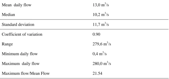
Table 1 reproduces the statistical parameters for the daily flows of Tirgua river at Paso Viboral gauging station during the period 1963-1993. Figures in the table indicate that daily flows show very high variations during the analyzed period. For a mean value of 13 m3/s and a standard deviation of 12 m3/s, coefficient of variation is 0.90; range is 280 m3/s; the relation between maximum and mean value is 21.54. This is a typical behavior for a mountainous river.
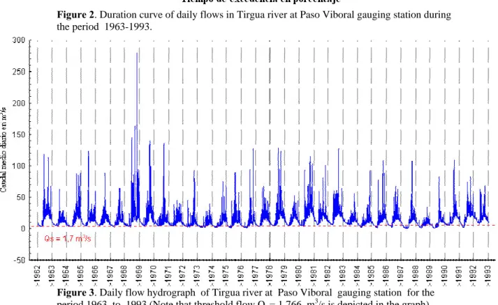
Flow duration curve is given in Figure 2. Flow values bigger than 20 m3/s are less frequently exceeded (time of exceedence less than 25 %), meaning that extreme high daily flows are of the rare occurrence. This fact can be also observed in daily flow hydrograph presented in Figure 3.
Table 1. Statistical parameters of daily flows in Tirgua river at Paso Viboral gauging station
during the period 1963-1993.
Mean daily flow 13,0 m3/s
Median 10,2 m3/s
Standard deviation 11,7 m3/s
Coefficient of variation 0.90
Range 279,6 m3/s
Minimum daily flow 0,4 m3/s
Maximum daily flow 280,0 m3/s
Figure 2. Duration curve of daily flows in Tirgua river at Paso Viboral gauging station during
the period 1963-1993.
Figure 3. Daily flow hydrograph of Tirgua river at Paso Viboral gauging station for the
period 1963 to 1993 (Note that threshold flow Qs = 1.766 m3/s is depicted in the graph).
Following the procedure indicated in the methodology threshold flow was estimated as Qs = 1.766 m
3
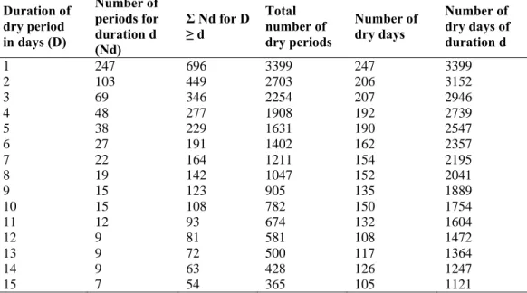
than this threshold value is considered as a dry day. The results are given in Table 2. The figures given in the table show a tendency to the occurrence of dry periods of short duration; at the most 30 days duration (with only one event). This is the reason because in Table 2 only the results for durations 0nee to 15 days are given. If the river maintains this hydrological behavior during 2006, there will be probably a water deficit in the supply system for San Carlos county.
Values given in Table 2 were adjusted to the exponential model. Parameter estimation as described in the methodology gave as result following model to estimate the number of dry periods as a function of duration:
d . 568 , 0 d 411,322.e n = − (4) R2 = 96,2 %; Se = 6,3 Where:
nd: number of dry periods
d: duration of the dry period in days R2: determination coefficient Se: Standard deviation of residuals
Table 2. Summary of results for the analysis of dry periods in Tirgua river at Paso Viboral
gauging station for the period 1963 - 1993.
Duration of dry period in days (D) Number of periods for duration d (Nd) Σ Nd for D ≥ d Total number of dry periods Number of dry days Number of dry days of duration d 1 247 696 3399 247 3399 2 103 449 2703 206 3152 3 69 346 2254 207 2946 4 48 277 1908 192 2739 5 38 229 1631 190 2547 6 27 191 1402 162 2357 7 22 164 1211 154 2195 8 19 142 1047 152 2041 9 15 123 905 135 1889 10 15 108 782 150 1754 11 12 93 674 132 1604 12 9 81 581 108 1472 13 9 72 500 117 1364 14 9 63 428 126 1247 15 7 54 365 105 1121
The high correlation coefficient (R = 0.981) and the relatively low standard deviation of the residuals validate de use of model (4) to estimate the number of dry periods in Tirgua river basin with sufficient precision. Nevertheless, it could be advisable to expand the research to other basins of the region and get other relationships by comparison of the results.
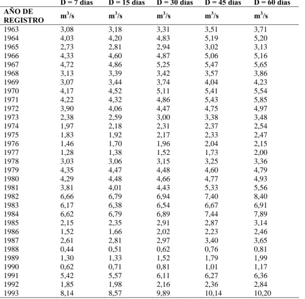
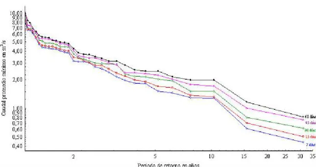
Using the procedure described in the methodology daily flow moving averages series for durations of 7, 15, 30, 45, and 60 days were constructed. The results are given in Table 4. On the basis of the values given in the table, frequency-duration analysis was done. The resulting Frequency-Duration Curves for Tirgua river flows at Paso Viboral gauging station for the period 1963-1993 are given in Figure 4. This standardized minimum flow analysis shows that the flow decreases with the recurrence interval for each duration following an exponential pattern. This allows to establish a unique mathematical
relationship to estimate the minimum flow for given period of returns and durations.
Using values of Table 3, model estimation parameter were adjusted and following results obtained for the model:
Table 3. Daily minimum flow moving averages of Tirgua river at Paso Viboral gauging
station for the period 1963 -1993. Durations of 7, 15, 30, 45 and 60 days.
D = 7 días D = 15 días D = 30 días D = 45 días D = 60 días
AÑO DE REGISTRO m3/s m3/s m3/s m3/s m3/s 1963 3,08 3,18 3,31 3,51 3,71 1964 4,03 4,20 4,83 5,19 5,20 1965 2,73 2,81 2,94 3,02 3,13 1966 4,33 4,60 4,87 5,06 5,16 1967 4,72 4,86 5,25 5,47 5,65 1968 3,13 3,39 3,42 3,57 3,86 1969 3,07 3,44 3,74 4,04 4,23 1970 4,17 4,52 5,11 5,41 5,54 1971 4,22 4,32 4,86 5,43 5,85 1972 3,90 4,06 4,47 4,75 4,97 1973 2,38 2,59 3,00 3,38 3,48 1974 1,97 2,18 2,31 2,37 2,54 1975 1,83 1,92 2,17 2,33 2,47 1976 1,46 1,70 1,96 2,04 2,15 1977 1,28 1,38 1,52 1,73 2,00 1978 3,03 3,06 3,15 3,25 3,36 1979 4,35 4,47 4,48 4,60 4,79 1980 4,29 4,48 4,66 4,77 4,93 1981 3,81 4,01 4,43 5,33 5,56 1982 6,66 6,79 6,94 7,40 8,40 1983 6,17 6,38 6,54 6,67 6,91 1984 6,62 6,79 6,89 7,44 7,89 1985 2,15 2,35 2,91 2,87 3,14 1986 1,52 1,66 2,02 2,23 2,46 1987 2,61 2,81 2,97 3,40 3,65 1988 0,44 0,51 0,62 0,76 0,81 1989 1,30 1,33 1,52 1,79 1,99 1990 0,62 0,71 0,81 1,01 1,17 1991 5,42 5,57 6,11 6,27 6,36 1992 1,85 1,98 2,16 2,36 2,84 1993 8,14 8,57 9,89 10,14 10,20
Figure 4. Frequency-Duration Curves for Tirgua river flows at Paso Viboral gauging station
for the period 1963 - 1993.
925 , 0 105 , 0 mín Tr D 053 , 5 Q = (5) R2 = 91,5 %; Se = 0,59 Where:
Qmín: minimum discharge of the river for a given period of return and a given
duration in m3/s D: duration in days
Tr: period of return in years R2: determination coefficient Se: Standard deviation of residuals
Since the coefficient of correlation is very (R = 0.96) and the standard deviation of residual very low, model (5) is suitable to estimate minimum discharges of the river for given return period and duration. Further studies should be done in neighborhood basins to check and validate the results and establish relationships for the whole region.
5. Conclusions and recommendations
From the obtained results following conclusions and recommendations can be drawn:
• There is a hydrological tendency in the river to the occurrence of dry periods of short duration in relation with the established threshold value.
• The number of dry periods in Tirgua river basin can be estimate with sufficient precision using the developed model given in equation (4). • To estimate minimum discharges of Tirgua river for given return
periods and durations the exponential model given by equation (5) can be used.
• Models (4) and (5) should be used only for preliminary studies at planning level.Further more it is recommended to validate the goodness of fit of the models as soon as new reliable basic information is available.
Acknowledgements:
Authors express the special acknowledgement following institutions for the partial financial support to this research :
1. Consejo de Desarrollo Científico y Humanístico, Universidad de Carabobo (CDCH-UC), Project No. 2005-009.
2. Coordinación de Investigación del Vicerrectorado de Infraestructura y Procesos Industriales. Universidad Nacional Experimental de los Llanos Ezequiel Zamora (UNELLEZ). Grant No. 31105101.
References
Carrillo, J., 1999: Agroclimatología. Editorial Innovación Tecnológica. CDCH – Universidad Central de Venezuela. pp. 213 – 246.
Dumith, D., Homes, P., Molina, G. y Peña, R., 1999: Plan de ordenación y manejo de la cuenca del río San Carlos. Documento de la Empresa Regional Desarrollos Hidráulicos Cojedes. Cojedes
Guevara, E.,1992: Métodos hidrológicos para el análisis de sequías. Ingeniería UC, 1(1), pp. 25-34.
Guevara, E., 2004: Modelación de los caudales mínimos en la cuenca del río Caroní. Proyecto de investigación subvencionado por el CDCH de la Universidad de Carabobo. Valencia, Venezuela.
Guevara, E. y Cartaya, H., 2004: Hidrología ambiental. CDCH-UC. pp 243 – 245. Guevara, E., 2005: Modelación de caudales ambientales en ríos de Venezuela.
Submited to Ingeniería UC.
Kiely, G., 1999: Ingeniería ambiental: fundamentos, entornos, tecnologías y sistemas de gestión (José Miguel Vza Trad.) Islas Gran Canaria, España: Mc Graw Hill. p. 279.
Montgomery, D., 1991: Diseño y análisis de experimentos. Grupo Editorial Iberoamericana. pp. 429 – 462.
Ojeda, R. y Espinoza, J., 1985: Análisis de los caudales mínimos en la región sur de Venezuela. Trabajo de grado de Ingeniería Civil. Escuela de Ingeniería Civil. Universidad de Carabobo, Valencia. pp. 22 – 37.
Rondón, G.,1988: Determinación de caudales derivables en épocas de estiajes en el río San Carlos – Sitio Paso Viboral. Documento del Ministerio del Ambiente y de los Recursos Naturales Renovables; Zona 8. Cojedes
Vide, J. 2000: Ingeniería Fluvial. Editorial Escuela Colombiana de Ingeniería. Colombia. pp. 77-138.