ADVANCED MICROGRID DESIGN AND ANALYSIS FOR FORWARD OPERATING BASES
by
ii
A thesis submitted to the Faculty and the Board of Trustees of the Colorado
School of Mines in partial fulfillment of the requirements for the degree of Master of Science. (Electrical Engineering) Golden, Colorado Date _______________________ Signed: _________________________ Jonathan Reasoner Signed: _________________________ Dr. P.K. Sen Thesis Advisor Golden, Colorado Date _________________________ Signed: _________________________ Dr. Atef Elsherbeni Professor and Head Department of Electrical Engineering and
iii DISCLAIMER
The views expressed in this academic research thesis are those of the author and do not necessarily reflect the official views, policy, or position of Colorado School of Mines, the United States Air Force, the Department of Defense, or the U.S. Government.
In addition, all images, figures, and data presented are unclassified and were gathered through the public domain.
iv ABSTRACT
This thesis takes a holistic approach in creating an improved electric power generation system for a forward operating base (FOB) in the future through the design of an isolated microgrid. After an extensive literature search, this thesis found a need for drastic improvement of the FOB power system. A thorough design process analyzed FOB demand, researched demand side management improvements, evaluated various generation sources and energy storage options, and performed a HOMER® discrete optimization to determine the best microgrid design. Further sensitivity analysis was performed to see how changing parameters would affect the outcome. Lastly, this research also looks at some of the challenges which are associated with incorporating a design which relies heavily on inverter-based generation sources, and gives possible solutions to help make a renewable energy powered microgrid a reality. While this thesis uses a FOB as the case study, the process and discussion can be adapted to aide in the design of an off-grid small-scale power grid which utilizes high-penetration levels of renewable energy.
v
TABLE OF CONTENTS
DISCLAIMER ... iii
ABSTRACT ... iv
TABLE OF CONTENTS ... v
LIST OF FIGURES ... vii
LIST OF TABLES ... ix
ACKNOWLEDGMENTS ... x
CHAPTER 1 - MICROGRIDS: DEFINITION AND APPLICATIONS ... 1
1.1 Literature Review and Previous Work ... 2
1.2 Motivation for the Research ... 4
1.3 Current Operating Procedures at FOBs ... 7
1.4 Hybrid Microgrid Design ... 8
CHAPTER 2 - MICROGRID DESIGN AND ANALYSIS ... 10
2.1 Case Study Description and Applications ... 11
2.2 HOMER® ... 12
2.4 Demand Side Management ... 16
2.5 Diesel Generator Modeling ... 19
2.6 Solar PV Power ... 20
2.7 Battery Storage ... 24
2.8 Converter Modeling ... 26
2.9 Wind Power, Fuel Cell, and Further DSM Discussion ... 26
CHAPTER 3 - SIMULATION PROCEDURES, RESULTS, AND ANALYSIS ... 30
3.1 Simulation Procedures... 30
3.2 Results and Discussions ... 31
3.2.1 Verification of Insulation Savings ... 31
3.2.2 Hybrid Microgrid Design and Analysis ... 33
3.3 Sensitivity Analysis ... 39
3.3.1 Adjusted Mission Length ... 40
3.3.2 Removal of Footprint Constraints ... 41
3.3.3 Adjusted FBCF ... 41
3.3.4 Adjusted PV Pricing ... 43
vi
4.1 Non-Dispatchable Generation Sources ... 45
4.2 Microgrid Protection Challenges ... 46
4.3 PV Panel DC Side Protection ... 51
4.4 Inverter Interconnection ... 53
4.5 Power Quality Issues ... 56
4.6 Flywheel Inverter System... 59
4.7 Electric Vehicle Energy Storage ... 60
4.8 Summary of Challenges and Future Work ... 63
CHAPTER 5 CONCLUSION, CONTRIBUTION, AND FUTURE WORK ... 64
5.1 Conclusion ... 64
5.2 Contribution ... 66
5.3 Future Work ... 67
REFERENCES CITED ... 69
APPENDIX A: HOMER MODEL INPUT PARAMETERS ... 74
APPENDIX B: COMPLETE HOMER ® SOLUTION REPORT ... 85
vii
LIST OF FIGURES
Figure 1.1 Literature Review Timeline ... 3
Figure 1.2 Current FOB Power Distribution System ... 7
Figure 2.1. Afghanistan Map ... 10
Figure 2.2. HVAC load from for 1 January ... 14
Figure 2.3. Daily operational load profile ... 15
Figure 2.4. Combined daily load for January 1st ... 16
Figure 2.5. Concrete Canvas FOB Structures ... 17
Figure 2.6. A Polyurethane Foam Insulated Tent ... 10
Figure 2.7. FOB Daily Load Profile with Foam Insulation Considered ... 18
Figure 2.8. Cummins MEP-012A V-12 Diesel Generator ... 19
Figure 2.9. Global Horizontal Radiation at the FOB Location ... 22
Figure 2.10. Comparison on PV Panel Types for Pricing Determination ... 24
Figure 2.11. The Tesla Powerwall® ... 25
Figure 2.12. Tesla PowerWall® HOMER® specifications ... 26
Figure 2.13. Initial Load Demand Example ... 27
Figure 2.14. Peak Shaving Process ... 28
Figure 2.15. Peak Shaving Result ... 28
Figure 2.16. Load smoothing using BESS ... 29
Figure 3.2.1. Bar Chart Comparison of the Solution Costs ... 34
Figure 3.2.2. Hybrid Design Cash Flow Diagram ... 35
Figure 3.2.3. Monthly Energy Production of the Solution ... 36
Figure 3.2.4. Final Solution PV Output DMap ... 37
Figure 3.2.5. Final Solution Diesel Generator Output DMap ... 37
Figure 3.2.6. The Solution Load Vs. Demand Diagram ... 38
Figure 3.2.7. Cash Flow Summary for the Base Case. ... 39
Figure 3.2.8. Cash Flow Summary for the Solution ... 39
Figure 3.3.1. Cost of Energy as Mission Length Increases ... 40
Figure 3.3.2. Sensitivity Analysis Results for the FBCF ... 42
Figure 4.1. Fault Current Contribution of a 1kW Inverter ... 47
Figure 4.2. Fault Current Calculation in PV String ... 52
viii
Figure 4.4. Droop Control Characteristics ... 56
Figure 4.5. Simplified Schematic of a Flywheel Converter ... 60
Figure 5.1. Simplified One-Line Diagram of the Recommended Solution ... 65
Figure A.1. PV Panel Cost Inputs ... 74
Figure A.2. Battery Cost Inputs ... 75
Figure A.3. Battery Property Inputs ... 76
Figure A.4. Inverter Inputs... 77
Figure A.5. MEP-012A Diesel Generator Inputs... 78
Figure A.6. System Load Inputs ... 79
Figure A.7. Solar Irradiance Inputs... 80
Figure A.8. Temperature Inputs ... 81
Figure A.9. Diesel Fuel Inputs ... 81
Figure A.10. System Control Inputs ... 82
Figure A.11. System Constraints Input ... 83
Figure A.12. Economic Inputs ... 83
Figure A.13. Emission Inputs ... 84
Figure B.1. Cost summary ... 86
Figure B.2. Annualized Costs ... 87
Figure B.3. Monthly Average Electric Production ... 88
Figure B.4. PV Output Data map ... 90
Figure B.5. MEP-012A Output Data Map ... 91
Figure B.6. Battery State of Charge ... 93
Figure B.7. Battery Monthly Statistics ... 93
Figure B.8. Battery SOC Data Map ... 94
Figure B.9. Inverter Output Data Map ... 95
Figure B.10. Rectifier Output Data Map ... 95
Figure C.1. MEP-012A Cummins V-12 Diesel Generator ... 96
ix
LIST OF TABLES
Table 1.1 Various RE/AE power generation and storage devices ... 8
Table 2.1. FOB Monthly Irradiance Averages... 21
Table 3.2.1. Insulation Verification Results ... 32
Table 3.2.2. Insulation Verification Analysis ... 32
Table 3.2.3. Simulation Results Comparison... 33
Table 3.2.4. Simulation Results Analysis ... 34
Table 3.3.1. FBCF Sensitivity Analysis Results ... 42
Table 3.3.2. PV Panel Cost Factor Sensitivity Analysis Results ... 43
Table 3.3.3. Battery Sensitivity Analysis Results ... 44
Table 5.1. Final Solution Cost Breakdown by Component ... 65
Table B.1. System architecture ... 85
Table B.2. Cost summary... 85
Table B.3. Net Present Costs ... 86
Table B.4. Annualized Costs ... 87
Table B.5. Electrical ... 88
Table B.6. Electrical Load ... 88
Table B.7. Load Met ... 89
Table B.8. PV Installed Ratings ... 89
Table B.9. PV Outputs ... 89
Table B.10. MEP-012A Operation ... 90
Table B.11. MEP-012A Output ... 90
Table B.12. MEP-012A Fuel ... 91
Table B.13. Battery Sizing ... 91
Table B.14. Battery Costs ... 92
Table B.15. Battery Storage ... 92
Table B.16. Converter Capacity... 94
Table B.17. Converter Operation ... 94
Table B.18. Emissions Output ... 95
Table C.1. Tesla PowerWall Lithium-Ion Battery System ... 97
x
ACKNOWLEDGMENTS
I would like to begin by thanking my academic advisor, Professor P.K. Sen, for his continuous support throughout my MS study program and thesis research. His guidance allowed me to not only complete this thesis, but gain a practical background in power systems analysis and design. His willingness to invest his time on his students allowed me to gain the best education possible. For that, I am extremely grateful.
I would like to thank Colonel Anne Clark (Department Head, Electrical and Computer Engineering, US Air Force Academy, CO) for providing me with the opportunity to attend graduate school, and Lt. Col. Paul Kaster (Ph.D. candidate, Colorado School of Mines, CO) for providing me with the contacts, constant guidance, and support required to succeed as a student at Colorado School of Mines.
Additionally, I would also like to thank my remaining committee members for taking valuable time out of their day to review, critique, and improve the work which I have done throughout this thesis.
1
CHAPTER 1 - MICROGRIDS: DEFINITION AND APPLICATIONS
The word microgrid has been used often in recent literature pertaining to electric power systems, many times without a clear definition of what a microgrid is. Microgrid is a general term used to define an electrical sub-system (big or small) consisting of interconnected loads and distributed generators. There is no exact definition of the size associated with a microgrid, either geographically or power consumption based, but widely accepted standards put into place by the U.S. Department of Energy defines them as systems consisting of less than 10MVA of load [3]. Microgrids consist of at least one Distributed Generator (DG) and typically at least one Distributed Storage (DS) unit, and can operate either connected to the larger grid, or electrically isolated as an island [1, 2]. A microgrid is often characterized by having an interconnection switch which is able to operate upstream of the microgrid in order to isolate the system from the larger utility. The DG & DS must be able to carry full or partial load within acceptable voltage and frequency variation limits. The microgrid must have protection, monitoring and control capabilities of all units within its area of responsibility as well.
Microgrid operating voltage levels depend on applications. A system covering a large geographic area of several square miles can operate at medium voltage (12.47kV – 69kV) levels commonly seen in distribution and sub-transmission systems, but microgrids that cover smaller areas, such as a single building, may operate at voltage levels as low as 120V. In addition, a microgrid can consist of a DC sub-system.
Distributed Generators (also sometimes referred as Distribution Energy Resources or DER) comes in a variety of types and sizes to fit the requirements of the microgrid. Renewable energy sources, such as photovoltaics (PV), are commonly associated with microgrid design, but
2
are not essential. A microgrid can be as simple as a single building with a diesel generator providing backup power if the larger grid fails, or as complex as a small town generating power from renewable sources and distributed storage throughout. This renewable source integration is an important aspect because it is critical to offsetting the capital cost required in transitioning a system into a microgrid design. Using a microgrid, more renewable sources and DG can be
utilized and the overall cost of customer’s electric bill can be decreased, helping to payback the
cost of system reconfiguration and the large amounts of capital typically needed.
1.1 Literature Review and Previous Work
Work on this microgrid applications topic really began to gain traction less than a decade ago. In 2007, Colonel Gordon Kuntz and Mr. John Fittipaldi published their work on behalf of the Army Environmental Policy Institute (AEPI) and the U.S. Army War College (USAWC). This work focused on identifying institutional impediments which were, at that time, preventing the Army from utilizing renewable energy sources [1]. Later, in 2009, the U.S. Army published the conclusions of their 2003-2007 research regarding casualty loss in attempts to locate high
risk areas and begin the mitigation process. This project, publish under the title “Sustain the Mission: Casualty Factors for Fuel and Water Resupply Convoys,” identified heavy losses which
are inflicted during fuel and water resupply [11].
In June of 2010, both Colonel John Vavrin and Dr. Amory Lovins published work which
aimed to advance research and place focus on the U.S. military’s need to improve their methods
for the generation of power on military FOBs. Colonel Vavrin, working out of the Construction Engineering Research Laboratory (CERL) in Champaign, IL, published his report which focused on methods in which energy demand could be reduced [9]. At the same time, Dr. Lovins
3
further explain the need for improvements. This paper focused on economic justification as well as vulnerability reduction for the military [8].
Soon after, in August of 2010, 2nd Lieutenant Nathan McCaskey of the U.S. Air Force published his research which performed a thorough economic analysis and ran simulations in an attempt to predict the effects that renewable energy source incorporation might have on not just the economics, but the casualty rates [23].
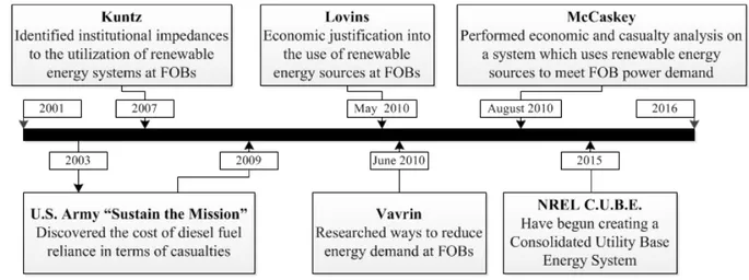
Since 2010, many entities have begun work on creating a practical system. In January, 2014, The National Renewable Energy Laboratory (NREL) and Georgia Tech have partnered up on a $2.9M sponsored by the Department of Defense (DoD) [71]. Hundreds of private companies have begun researching and testing solutions, and various government laboratories and organizations have invested in the design of a better method for meeting the power requirements of a forward operating base. This information is shown below in Figure 1.1.
Figure 1.1. Literature Review Timeline. This summarizes work done on this topic up to the thesis start date.
4
1.2 Motivation for the Research
One of the most researched applications of microgrid technology in North America is for the military applications. The United States Department of Defense (DoD) spends $2.2 billion per year on electricity, largely purchased from local utilities. The National Defense Authorization Act of 2010 requires the DoD to ensures that at least 25% of energy consumed comes from renewable sources. This requirement boosted investment in clean energy technologies as well as microgrid studies and pushed a program called SPIDERS to the front on the microgrid race [4, 5].
The Smart Power Infrastructure Demonstration for Energy Reliability and Security (SPIDERS) program is sponsored by the Department of Defense in collaboration with the Department of Energy (DoE) and Department of Homeland Security (DHS) to create a cyber-secure microgrid design which would have the capability to supply critical loads in the event of a power outage of the local utility. The three phases consist of a single building microgrid, a portion of a base with microgrid architecture, followed by the development of a microgrid for an entire military installation. This program, which is currently in phase 3, is leading the way and learning valuable lessons regarding microgrid design and implementation [5, 6]. Military applications are not the only worthwhile use for microgrids. Data centers, hospitals, and college campuses all require very high reliability (very close to 100%) due to data availability, healthcare requirements, and research.
A microgrid would allow the ability to have an ensured source of power and be able to do it while intelligently utilizing locally viable renewable energy sources. It could do this while providing lower energy costs to the consumer through the use of renewable energy sources and systems with higher efficiencies. Higher efficiency may be attained in microgrids because of the
5
smaller distance and fewer devices which the power must travel through in order to reach the consumer. Many of these ideas are being researched heavily and they are in cutting edge of the technology.
While microgrids for permanent (Garrison) facilities are beneficial in many ways, this thesis will investigate the application of microgrids for Forward Operating Bases (FOBs). A FOB is a remote temporary military base which houses a small number of military personnel (typically several hundred to several thousand) and has a tactical and operational focus in the fighting of the military conflict at hand. The base footprint is typically around 1 square mile and consists of temporary or semi-permanent structures, and lacks most amenities seen at permanent military locations. For obvious reasons, improving the power system at these facilities is an extremely critical requirement. Modern military combat, which is increasingly centered around a traditional military engaging an insurgent force exacerbates the weakness of supply lines due to the lack of a conventional battlefront. This allows enemies to slip behind the fighting forces and attack the lightly armored supplies lines bringing food, water, fuel, ammo, and medical supplies to the soldier’s FOBs.
Modern military FOBs rely almost exclusively on diesel generators to supply power, a
practice which requires the military to pay “high costs in blood, treasure, and combat
effectiveness” [8]. The fully burdened cost of fuel (FBCF) represents not only the price paid per gallon of fuel, but the cost incurred delivering that fuel to its destination [10] and associated loss of human life and property. There is no standard method for calculating this cost, and estimates vary drastically between $15 and $400 per gallon of diesel.. It has been shown that for every gallon of diesel delivered to a FOB, it takes up to seven gallons to get it there for Operating Enduring Freedom (OEF). This leads many researchers to a common estimated fully burdened
6
cost of fuel (FBCF) to be between $15-20/gallon (2013 data) [9, 10]. This thesis will follow the assumption of [8], [9], and [23] in assuming the FBCF to be $17.44, but a sensitivity analysis will be performed to show the effects of a changing FBCF. It is very important to note that these figures are extremely difficult to calculate accurately and quite often different sources will take different factors into account. Needless to say, the cost is very high regardless of assumptions. A simple check on the estimate was to consider the current price of a gallon diesel ($2.50) and assume that it takes the average of seven gallons to deliver that to the operating base. If these were the only factors considered (the most simple method of FBCF calculation), the FBCF would be ∗ $ . /�� = $ . /�� . This number very closely correlates with the $17.44/gallon figure used by previous researchers. This thesis did not consider the changing price of diesel fuel, but rather assumed that it stayed constant throughout the mission.
In addition the material cost, supply convoys carrying fuel account for between 10%-20% of the casualties seen in Afghanistan [11]. The U.S. Army has shown that between the years of 2003-2007, an average of one out of twenty-four fuel convoys sustained casualties. By
decreasing the number of fuel convoys, you decrease the number of soldiers placed in harm’s
way for the sole purpose of delivering fuel intended for electricity production [11].
These reasons give clear motivation for diminishing the U.S. military’s dependence on only diesel powered generators. In order to save lives and resources, the US military must find better and smarter ways to provide reliable and sustainable power to FOBs. This is no easy task. There are many challenges associated with the use of hybrid power systems including renewable energy sources discussed at length in this research. This thesis will delve into issues dealing with some of these challenges and how they apply to an example of a future FOB power system.
7
1.3 Current Operating Procedures at FOBs
The amount of power required at a FOB is calculated based on the mission type and the number of personnel at the base. The process for determining the number of generators required involves using a lookup table with the equipment and facilities which will be deployed, and adding to this the product of the number of soldiers and their mission type. This is estimated between 3-6kW per person at Army or Air Force installations, depending on the location and mission [7]. This figure is often robustly calculated, leaving an average demand factor of 30%, and an average operating generator loaded at 80% [9]. For a base comparable to that which is being studied, six to eight 750kW diesel generators would be used. The electric distribution
system would consist of a minimum of two geographically separated “power plants” which are
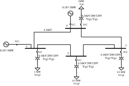
comprised of these diesel generators connected into a looped 4.16kV distribution system. Transformers would step the distribution voltage levels down to the 277/480V or 120/208V or 120-240 1-phase radial feeders, allowing the power to be consumed. This is shown below in Figure 1.2. 1 2 3 4 0.187-3MW N.C. N.C. N.C. N.C. N.C. 1MW .9 pf 0.5 MW 0.9 pf 1 MW 0.9 pf 0.5 MW 0.9 pf 0.187-3MW N.C. 4.16kV 4.16kV/208/120V Y(g)-Y(g) 4.16kV/208/120V Y(g)-Y(g) 4.16kV/208/120V Y(g)-Y(g) 4.16kV/208/120V Y(g)-Y(g)
Figure 1.2. Current FOB Power Distribution System. This is a simplified one-line diagram of a non-specific FOB power distribution system.
8
1.4 Hybrid Microgrid Design
The current method for power generation at a FOB is essentially the same method used for the last century, and it is due for an overhaul for multiple reasons. One possible solution is a hybrid microgrid power system. A hybrid microgrid is a small electric grid which utilizes generation sources of various types in order to meet the demand. Because of the intermittent nature of renewable energy sources, the interconnection of dispatchable and non-dispatchable resources is important to ensure that reliability rates remain high as renewable energy sources are utilized in the system [45]. If generator sizing is properly performed, reliability rates can remain high while system efficiency can be increased and fossil fuel consumption can be reduced a lot. Table 1.1 below gives a short list of renewable energy (RE) and alternative energy (AE) technologies, along with current energy storage solutions.
Table 1.1 Various RE/AE power generation and storage devices [45].
Much of the challenge in creating a hybrid microgrid occurs because of the differing operating procedures of the various renewable energy sources. The ideal hybrid design would be capable of incorporating new energy sources without system reconfiguration, a capability
9
of interconnection are being used. These methods include DC-coupled in which the sources are interconnected on the DC side of an inverter, AC-coupled where the inverters convert DC to AC and then each source is connected using transformers, and hybrid coupling where both methods are used in a single system [46].
Currently, Air Force research is leaning away from battery storage solutions and more towards grid-tied PV systems due to the added complexity in communications and system operation required. Despite this, this thesis will analyze the benefits of including the BESS into the system design.
10
CHAPTER 2 - MICROGRID DESIGN AND ANALYSIS
Proper and efficient hybrid design of a microgrid requires extensive knowledge of multiple disciplines and parameters. This chapter investigates the design and analysis of a FOB located in Southern Afghanistan. This FOB being studied is assumed to be occupied by 1,100 airmen, a common size for Air Force FOBs, and has a slightly above average solar irradiance level and slightly below average wind speed when compared to the rest of Afghanistan. The general location is given as southern Afghanistan. These values for average irradiance and wind speed are 5.74 kWh/m2/day and 4.56m/s at 50m, respectively [23].
Figure 2.1. Afghanistan Map. The FOB studied in this thesis looked into a base located in the southern portion of Afghanistan [72].
11
This is an interesting and useful site to study because it is similar to other regions in Afghanistan, a region where U.S. military operations are ongoing. The FOB being studied is in an isolated area of Afghanistan with limited supply routes, making the delivery of fuel a dangerous endeavor. This area has comparable weather to that seen in Iraq and throughout the Middle East, making many of the assumptions valid for other areas as well. The electrical load was first estimated, then current techniques for supplying the loads with power were modeled to give a baseline of comparison. After the baseline was calculated, a design incorporating solar (PV) energy and battery storage was tested and calculated. Lastly, a comparison was made with the existing design and recommendations are given. In addition, a literature review into current methods available to decrease the demand was performed and several promising solutions were developed.
2.1 Case Study Description and Applications
This thesis will propose and analyze a microgrid design for a U.S. Air Force FOB of 1,100 airmen located in southern Afghanistan. This hybrid microgrid design will attempt to decrease demand for diesel fuel, while maintaining system reliability. Assumptions which will be made for this thesis include are that the cost of fuel will remain constant of the mission length of five years. This thesis will also assume that there is no load growth over the mission length.
This thesis looks into not only a specific design for one location, but a generic method for designing for cost effective solutions for the electrical power system for an isolated microgrid. Specifics factors considered include costs of military operations, the fully burdened cost of fuel, strict reliability requirements, and a need for robust, over-engineered solutions.
While this thesis was designed with military applications in mind, there are many applications beyond the scope of Forward Operating Bases. The problems addressed in this
12
issue are common to virtually all isolated microgrids which are currently being researched. Only the specific solution provided in later chapters relates to the FOB, the methodology and
discussion is universal to all other microgrids.
2.2 HOMER®
Hybrid Optimization of Multiple Energy Resources (HOMER®) is a computer program developed by NREL to aid in microgrid design, analysis, comparison, and economic analysis. Some would not classify it as a true optimization program, because it only performs calculations based on discrete and specific data input by the user, but for this case, it was used to find the ideal combination of generation units out of the thousands of combinations available. The way this program works is the user to determine a base load, fixed generator costs, fuel costs,
renewable resource availability, and incremental amounts of generation sources - and HOMER® then calculates and organizes the results based on the cost. In addition to generation level search spaces, sensitivity analysis can be performed to see how changing of variables, such as diesel fuel price or PV panel installed cost, will affect the solutions.
HOMER® is a powerful calculation tool which takes into account many factors such as battery capacity loss over time, sub-optimal generator loading’s effect on efficiency, PV cell
temperature’s effect on PV panel output, average cloud cover (clearness index), and even salvage
cost for generation equipment.
2.3 Load Analysis
Power demand requirements at Forward Operating Bases can be classified into two main categories. The first category is the operational power requirement. This is the power requirement which is critical to maintain operations. It includes security, communications,
13
cooking, lighting, and many other essential loads. The second category is the power required for the heating, ventilation and air-conditioning (HVAC) of the structures and tents. These two loads are signified as and ℎ for the remainder of this thesis. McCaskey has laid out much of the ground work for modeling the load of a FOB in [23] and developed the following equations based on estimates, as there is no real data for actual FOB power consumption available. This is discussed later in Section 4.9.
(2.1)
= . cos � + , . � (2.2)
(2.3)
(2.4)
Where, t is the time of the day and T is the temperature.
Equation 2.1 shows that the total power demand is equal to the sum of the operational load and the HVAC system. The HVAC system demand model is used based on the recommendations of [23] with one major exception. Rather than using the temperature equation calculated in [23], this thesis used empirical data was used from Tucson, AZ. Tucson, AZ is a reasonable estimation of the weather at FOB site selected for this thesis, the altitudes are just 47m difference, and the Latitude is just 0.72ᵒ difference. In addition the average solar irradiance at the FOB is 5.74kWh/m2/yr, while the recorded average for Tucson, AZ is 5.70kWh/m2/yr, based on available solar irradiance data provided by the National Renewable Energy Laboratory
ℎ , = { − . + . , < . . , . ≤ ≤ . . − . , > . ℎ , � ℎ = { − . + . , < . , ≤ ≤ . − , > = + ℎ
14
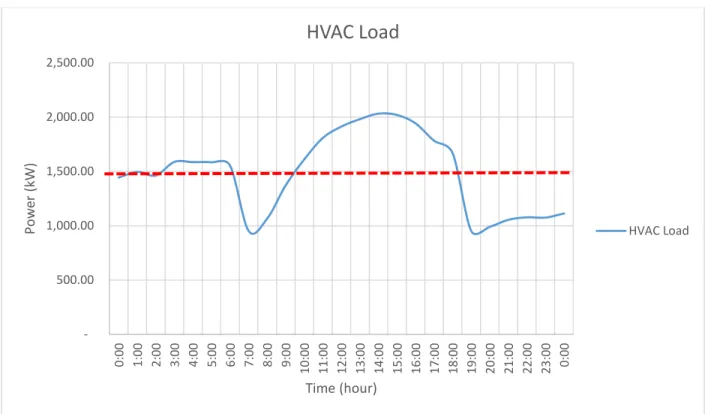
(NREL) [30]. A plot of the HVAC load is shown below in Figure 2.2 for a time period of 24 hours, starting at 0000 on January 1st.
Figure 2.2. HVAC load from for 1 January. This plot was created in Excel based off of Equations 2.3 and 2.4, over a 24 hour period.
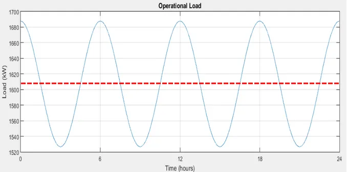
The operational demand was calculated using [23]-[25], assuming a force size of 1,100 airmen, as stated earlier. The load equation is a sinusoidal function which correlates the maximum demand to the meal times due to the extra load of the kitchen equipment. These times are at 0000, 0600, 1200, and 1800 hours. While doing further analysis, it is clear that the actual fluctuation is very minimal (about 5% (= ∗ .
, . ) from the constant load. This is shown
below in Figure 2.3. 500.00 1,000.00 1,500.00 2,000.00 2,500.00 0:00 1:00 2:00 3:00 4:00 5:00 6:00 7:00 8:00 9:00 10:00 11:00 12:00 13:00 14:00 15:00 16:00 17:00 18:00 19:00 20:00 21:00 22:00 23:00 0:00 Po w e r (kW) Time (hour)
HVAC Load
HVAC Load15
Figure 2.3. Daily operational load profile. The plot was created using MATLAB® and is based off of Equation 2.2.
The yearly load was calculated by taking the sum of and ℎ at one-hour intervals. This revealed a maximum demand of 4.568MW and a minimum demand of 2.602MW over the course of a year. The load factor was calculated to be 0.7. Load factor (LF) is defined as the ratio of the average demand seen in the system for a specified period to the maximum demand seen for that same period of time, as shown below in Equation 2.5. Ideally, this number should be as close to one as possible, meaning that the average load is the maximum load and that there is no load variation present in the system.
. �. =� �� (2.5)
An example of the daily load profile is shown below in Figure 2.4 for January 1st. Additionally, the capacity factor was calculated to be 0.533, based on an average daily energy demand of 76,732kWh/day and eight 750kW MEP-012A diesel generators being available for dispatch.
16
Figure 2.4. Combined daily load for January 1st. This figure represents the combination of Equation 2.2 through 2.4, as defined in Equation 2.1.
Figure 2.4 shows a typical daily load cycle, this value does not reach the maximum demand mentioned in the previous paragraph because it is during a day which lacks heavy HVAC requirements. The maximum demand occurs on 23 June at 1500 hours.
In order to check this for accuracy, the maximum demand was divided by the number of soldier at the FOB. The result of this calculation ( , �
, � = . �/�� � ) show that
our calculations are right in-between the typical 3kW-6kW “rule-of-thumb” calculations described previously. This proves that a reasonable assumption for what the load will look like for the FOB has been calculated for use by this thesis.
2.4 Demand Side Management
The next step was to look how an overall FOB design can be changed in order to decrease the demand, and/or increase the demand factor. These considerations are commonly classified as
500.00 1,000.00 1,500.00 2,000.00 2,500.00 3,000.00 3,500.00 4,000.00 P o w er ( k W) Time (hour)
Daily FOB Load Profile
HVAC Load Operational Load
17
demand side management (DSM) improvements. Once and in-depth knowledge of the demand has been gathered, changes can be made to the load which allows for saving of fuel and the decrease in equipment required. The first area which will be looked at is decreasing the demand.
The obvious area which should be analyzed in order to decrease the load demand is the inefficient structures which are utilized on forward operating bases. As much as 75% of the electrical demand is required by the HVAC systems for operations in the Middle East. Of this energy, as much as 50% is lost due to the thin skin tents used, which do not have insulation or enough thermal mass in them [9]. Two techniques which are currently being tested involve increasing the thermal mass and increasing the thermal resistivity.
In order to increase thermal mass, a new type of structure is being developed which consists of fabric which is filled with concrete. This structure, which resembles a tent initially is erected by inflating it with air, and then sprayed with water, causing the concrete to set. This structure can then be covered in soil which increases its thermal mass and allows for increased insulation properties, while also providing protection from small arms and indirect fire. This structure is shown below in Figure 2.5.
Figure 2.5. Concrete Canvas FOB Structures. This concrete inflatable tent alternative which is possesses a higher thermal mass and will decrease the HVAC load requirement at FOBs [44].
18
The second method utilizes a spray on foam covering over the tents. Adding the six to twelve-inch thick polyurethane foam layer to the tent, as shown in Figure 2.6 can reduce HVAC demand anywhere from 33%-50% [41].
Figure 2.6. A Polyurethane Foam Insulated Tent. This spray foam covers existing tents to help insulate them from heat loss, leading to a reduction in power demand ranging from 33% to 50%
[42].
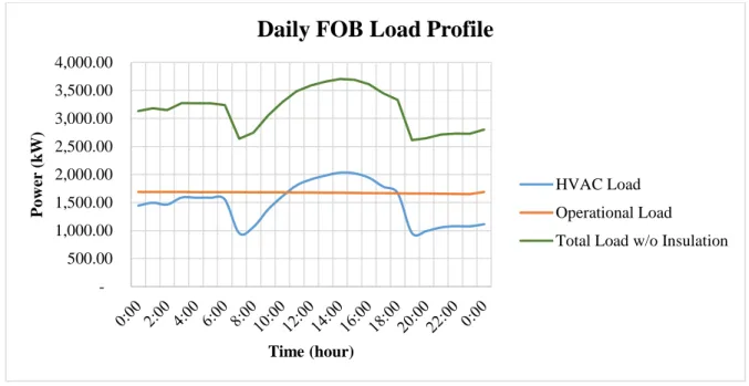
Because of the availability of data from tests in both Afghanistan and Iraq, this thesis will include the HVAC insulation into the system design. The results of including this 33% reduction in HVAC load is shown below in Figure 2.7.
Figure 2.7. FOB Daily Load Profile with Foam Insulation Considered. This was created using Excel and takes into account the effect of foam insulation on the daily energy demand.
1,000.00 2,000.00 3,000.00 4,000.00 P o w er ( k W) Time (hour)
Daily FOB Load Profile
HVAC Load Operational Load
Total Load with Insulation Total Load w/o Insulation
19
The combined load factor with the foam insulated considered was calculated to be 0.748. Additionally, the adjusted capacity factor was calculated to be 0.447, based on a reduced average daily energy demand of 64,313kWh/day and eight 750kW MEP-012A diesel generators still being available for dispatch.
2.5 Diesel Generator Modeling
In order to calculate the baseline operating costs, it was assumed that MEP-012A, diesel powered AC generators were used [24] (data sheet given in Appendix C, also shown below in Figure 2.8). It was also assumed that each generator was loaded equally, and spinning reserve was not considered. This means that if 3,200kW of power was needed, 5 generators were loaded to 640kW each. Fuel consumption rates were assumed to be a linear relationship between the idle consumption rate and the full load consumption rate. These values were given in [24].
Figure 2.8. Cummins MEP-012A V-12 Diesel Generator. This diesel generator is the standard generator used by U.S. military forces to meet energy demand on FOBs[25].
20
Over the course of a year, this thesis calculated the total cost of electric power production to be $35.47 million dollars. That is very close to the results obtained in [23] which calculated $33.7 million and [8] of $34 million. The difference may be due to the use of actual data points for the temperature rather than a mathematical equation based on the monthly high and low temperatures, which was the method used in [23]. Another possible source of error is assuming that each generator is equally loaded, rather than all but one generator loaded to the maximum amount. When generators operate at rated output, fuel efficiency increases, therefore decreasing the fuel costs over the course of a year.
The price of a MEP-012A diesel generator was set to $240,000 (as specified in [23]) with a replacement cost of $70,000 for the generator overhaul which is required after 10,000 hours of operation. The Operation and Maintenance (O&M) cost is set to $2.40/hr [31], [23]. In addition, shipping costs for the generator sets is set at $1.50 per pound. With a dry weight of 24,500lbs [24], that gives an additional cost of $36,750 per generator.
As discussed previously, the fuel cost used in this project was $17.44/gallon of diesel.
2.6 Solar PV Power
The FOB is in a suitable location which allows for the generation of electricity and utilization of PV resources. Utilizing this resource is advantageous because PV panels do not require additional personnel for maintenance, they are static, and silent. As a starting point for analysis, this thesis assumes that each structure is capable of handling the weight required to support the PV panels. Based on [23]-[25], 9,400m2 of usable surface area is present on which PV panels can be mounted atop of structures for the FOB. For this simulation, it is also assumed that only 80% of that surface was usable. The solar panels are assumed to have 18% efficiency
21
[28] and the assumption was also made that the solar panels placed above the structures does not have any effect on the HVAC requirements.
This would yield about 1.67MW of available peak solar capacity which can be installed. In addition to the 1.67MW of rooftop solar, it is assumed that a maximum of 3.33MW of ground placed solar panels is possible. This gives HOMER and search space from 0MW – 5MW of PV panels. The calculations will have a resolution of 50kW, meaning that there are 100 possible power rating of PV which will be analyzed.
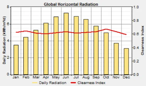
The data used to simulate the solar irradiance seen by the panel was collected by NASA [30] and verified through the Air Force research [31]. The monthly average for solar irradiance is given below in Table 2.1 and Figure 2.9.
Table 2.1. FOB Monthly Irradiance Averages. This table represents the average global horizontal irradiance seen for the specific location of the FOB [30].
Month Irradiance Units
Jan
3.5 kWh/m
2/d
Feb
4.43 kWh/m
2/d
Mar
5.27 kWh/m
2/d
Apr
6.08 kWh/m
2/d
May
6.86 kWh/m
2/d
Jun
7.28 kWh/m
2/d
Jul
6.89 kWh/m
2/d
Aug
6.52 kWh/m
2/d
Sep
5.76 kWh/m
2/d
Oct
4.94 kWh/m
2/d
Nov
3.71 kWh/m
2/d
Dec
3.08 kWh/m
2/d
22
Figure 2.9. Global Horizontal Radiation at the FOB Location. This graph, created by HOMER® and verified using USAF research gives the irradiance seen at the ground and the clearness
index.
This data gives an average irradiance of 5.364kWh/m2/day over the course of a year and
an average “clearness index” of 0.625. The clearness index is equal to the ratio of the irradiance
measured at the ground to the extraterrestrial irradiance seen at the outer-most part of earth’s atmosphere. This clearness index considers the average cloud cover, dust, atmosphere, humidity, and other factors which affect the travel of light to the surface of the earth.
The photovoltaic (PV) model uses several inputs in order to calculate the estimated output. The lifetime of the solar panel was specified as 25 years, which is the industry standard
[28]. The “derating factor” was set to 77%. This factor takes into account many issues
including the PV module nameplate DC rating, the inverter and transformer losses, the mismatch in maximum power point between true value and manufacturer specified point, the forward bias junction loss of diodes, and the wiring and connection losses. The choice of 77% was based on the suggested value given in [33]. In [33], a complete breakdown of each contributor for the
23
77% derating from can be found. The slope of the solar panels was set to the latitude of the location, 320. The solar panel azimuth was set to due south. Lastly, the ground reflectance was
set to the default value of 20%. The “ground reflectance” is the fraction of the solar radiation which is incident to the ground. The panels were selected to be “non-tracking”, and the effects
of temperature on the PV panel considered using average monthly temperatures obtained from [30].
An in-depth cost analysis of photovoltaic systems, both small and large scale, has been performed in [34] and [35]. The results of this gave a projected installation cost of $4,000/kW ($4/W), and an operation and maintenance cost of $0.019/W/year. It is important to note that this installation cost does include the inverter and other associated cost for control as part of the
photovoltaic system, but doesn’t include any battery storage. In addition, $1.50 per pound was
added to the cost for shipping to the destination and back after the mission has concluded. This comes to an estimated $1,200/kW ($1.2/W). After review, this $4/W value was found to be lower than seen currently. Future work should be performed to accurately incorporate the cost of mounting systems into the installed cost of PV panels. This project attempted to correct this through a sensitivity study which is discussed in Chapter 3.
When PV solar power is utilized on a military facility, there is the option to place it overtop of physical structures, in unused area, or to increase the base perimeter to allow for the additional space. In order to model this within HOMER®, the installed cost of PV was assumed to increase to $8,000/kW ($8/W) after all of the usable area on top of shelters was utilized. This additional cost estimation is to help offset the price of increasing the perimeter and the factors which accompany that. A comparison of solar panels which fit into the lower tier pricing vs. the
24
higher tier pricing is given below in Figure 2.10. It is assumed that PV has a footprint of 9.29m2 per kW [23]. This number will be used for feasibility analysis and system design [38].
Figure 2.10. Comparison on PV Panel Types for Pricing Determination. Figure 2.10(a) represents the type of solar panel which would fit into the lower tiered pricing, while Figure
2.10(b) represents the type of panel which would fit into the higher tiered pricing.
2.7 Battery Storage
Battery storage is a highly desired component for the effective integration of intermittent renewable energy sources in a hybrid design for FOB application. Since previous analyses were performed, there has been only one major development in energy storage solutions. This
breakthrough is due to Tesla’s new Powerwall®
battery storage system [26], which is shown below in Figure 2.11.
The Tesla Powerwall® sets a new, low price point with 10kWh storage systems costing only $3,500 for weekly cycling intended, and a 7kWh system designed for daily load cycling. With these new lowered price points, economic analyses are performed. This lowers the cost per kWh of energy storage from the typical value of $0.20 - $0.50 per kWhr to $0.10 to $0.12 per kWhr [27].
25
Figure 2.11. The Tesla Powerwall®. This Tesla Powerwall® battery energy storage system was sued at the energy storage system in this hybrid microgrid design [26].
While some specifics are not yet available, enough data is present in [29] to create a usable model of the PowerWall®. The price point for the Tesla PowerWall® battery is $3,500 for a 10kWh battery system, which has an output voltage of 400VDC. Also given is the maximum and nominal current output of the battery, the roundtrip efficiency, and an estimate of the cycles to failure [29]. These values were used to create the battery model shown below in Figure 2.12 and self-explanatory. The full specification sheet is given in Appendix C.
In addition to the cost of the battery, shipping costs of $1.50 per pound adds an additional $330 per battery. In addition to the shipping costs to bring the batteries to the area of operations, shipping costs to return them will be included as well. This adds an additional $330 per battery system, bringing the total cost to $4,160 per battery system.
26
Figure 2.12. Tesla PowerWall® HOMER® specifications. This was the battery input screen in HOMER® which was used to solve for the ideal solution.
2.8 Converter Modeling
The converter modeling in Homer® has an inverter efficiency of 95% [36] and a rectifier efficiency of 92% [37]. Because the inverter cost is included in the installed cost of the PV sources, all costs were set to 0.
2.9 Wind Power, Fuel Cell, and Further DSM Discussion
Wind power is not taken into account in this research work because of the requirements to elevate the generation units. This attracts attention and gives an easy target and reference point for any attack. In addition, the base is surrounded by thick walls which create turbulence and require addition height to be added to a wind turbine. A third reason is that the wind
27
turbines would be located near the FOB runway, causing both a physical obstacle as well as a source of turbulence for aircraft taking off and landing. There are, however, many applications for wind power at the Garrison level, and for many other non-military microgrids. That study is outside the scope of this thesis.
Fuel cells were deemed to not be a practical solution for this problem because of the lack of technological maturation. The cost of creating hydrogen, the complexity of transporting it, and the difficulty of storing it made it an ineffective solution to the problem at hand.
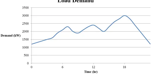
Further demand side management improvements to decrease and level the load are possible. By shifting the peak load to a time which experiences lower demand, load factor can be increased
An increase in demand factor (DF) means that fewer generators will need to be dispatched in order to meet the demand. This concept over decreasing the LF is referred to as peak shaving or load leveling, and is shown below in Figure 2.13- 2.15.
Figure 2.13. Initial Load Demand Example. This is an example load profile before any adjustments have been made.
28
Figure 2.14. Peak Shaving Process. This graphic showing the process of peak shaving through the relocation of demand from areas of high power demand to areas of low power demand.
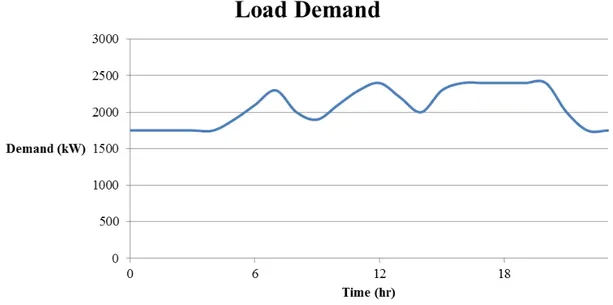
Figure 2.15. Peak Shaving Result. This represents the load profile after load smoothing has been performed.
In the example above, if the amount of generation available is assumed to be 5MW, the initial demand factor, according to Figure 2.12 would be �� = �
29
smoothing has been performed, assuming that the same amount of generation is available, the demand factor would be �� = �
�= . . This means that less generation is now required
to meet the demand, decreasing the capital cost of the system as a whole.
This demand side management technique of load factor improvement may prove to be difficult to perform for the FOB application. The majority of operational loads are considered critical and cannot be shed, leading only HVAC loads to be decreased throughout the day. One method for implemented this demand side management strategy without sacrificing power availability for any loads is to use the battery storage. By charging the battery energy storage system (BESS) during hours of low demand, and discharging the BESS during hours of peak demand, the load will be smoothed and less of the peak load must be met by generating units. This is illustrated below in Figure 2.16.
Figure 2.16. Load smoothing using BESS. This methods can be used to decrease the DF of a power system [47].
30
CHAPTER 3 - SIMULATION PROCEDURES, RESULTS, AND ANALYSIS
A HOMER® discrete optimization analysis was performed using the values described in Chapter 2. The goal was to determine if the decrease in fuel costs attained by the addition of PV and BESS was enough to offset the increase in capital cost. This chapter explains the
procedures, results, and provides a final recommended for the FOB power system design.
3.1 Simulation Procedures
The first step in the calculation was to determine the search space. HOMER® defines the search space as the maximum and minimum amounts of each generation or storage source. The amount of solar PV to be considered (search space) ranged from 0MW to 5MW, with the first 1.67MW (the effective area of covering all structures) utilizing the lower ($4/W) pricing and the remaining 3.33MW utilizing the higher ($8/W) pricing. The search space had a resolution (increment) of 50kW. The number of batteries included in the design was set to vary from 0 to 2,000, with a resolution (increment) of 50 batteries. Lastly, the number of generators was set to 7. This purpose for this was to include the cost that ensures power system reliability in the event of a long term lack of renewable energy or damage to the PV system. This allows the diesel generators to provide power for the full demand while repairs are made or the inclement weather passes.
Operating reserves were set to Homer default values with 10% of the hourly load or 25% of the solar output, whichever is greater.
The full set of input parameters for the Homer model is located in Appendix A for future reference. Three major sets of simulations were conducted as follows.
31
(1) The first simulation performed in HOMER® had the purpose of verifying the
reported cost savings of adding polyurethane foam insulation which were reported in [41] and [42]. This was done by comparing the base case without insulation, with the base case with insulation capable of decreasing demand by 33%.
(2) The next simulation performed was an optimization to determine the optimum
amounts of PV and BESS which should be included into the FOB (Hybrid) power system.
(3) The final simulations performed were sensitivity analyses which examined the effects
that a drastic increase in diesel fuel prices and PV panel installed costs would have on the cost-effectiveness of the solution.
3.2 Results and Discussions
This section will look into the results of HOMER® simulations which were performed. As mentioned previously, three simulation types were performed. These included (1)
verification of insulation savings, (2) the determination of the ideal solution, and (3) a sensitivity analysis of the ideal solution.
3.2.1 Verification of Insulation Savings
The addition of foam insulation increases the capital cost of the FOB power system. Based on the number of structures located at the FOB (given in [23] by HQ AFCESA/CEXX) and the reported cost of insulation (given in [42]) the estimated cost to insulate each structure at the FOB would total to $5M. Additionally, it was then assumed that the insulation would decrease the HVAC demand by 33%, as reported in [41] and [42]. HOMER® then simulated the base case (only diesel generators used to meet the demand). The results of this simulation are shown below in Table 3.2.1, where the first row is the base case, and the second row is the base
32
case with the introduction of foam insulation. Table 3.2.2 compares the maximum, average and minimum demand, along with the load factor and the percentage of the total load which is the result of HVAC.
Table 3.2.1. Insulation Verification Results. This is a comparison of results between the base case with and without foam insulation installed, where the upper row is the uninsulated case results, and the bottom row is the insulated case results. Neither of these consider renewable
energy generation sources.
Table 3.2.2. Insulation Verification Analysis. This is a simplified load analysis comparing the insulated and non-insulated case. Neither of these cases consider the addition of renewable
energy generation sources.
Table 3.2.1 shows a capital cost increase of $4.4M, a value less than the $5,000,000 previously mentioned. The reason for this variance is that the maximum base load is now able to be met using only five of the MEP-012A diesel generators. Results of this simulation point towards a payback time of between 7 and 8 months, significantly longer than suggested by private companies selling the product, who advertise a payback time of 29 days [42].
Diesel Price $ 17.44 $/gallon 33%
Maximum # of Utilized
Diesel Generators
Capital Cost Yearly
Operation Cost 5 Year Cost
Electricty Cost ($/kWh) Gallons of Diesel Consumed 7 $ 1,937,250.00 $ 36,958,296.00 $ 157,619,040.00 $ 1.336 2,089,877.98 5 $ 6,383,750.00 $ 30,014,142.00 $ 132,814,232.00 $ 1.343 1,699,945.32
Economic Evaluation of Adding Foam Insulation at the Marjah FOB Foam Efficiency Increase
Without insulation With Insulation % Difference Max Demand (kW) 4,568 3,583 -22% Avg Demand (kW) 3,198 2,680 -16% Min Demand (kW) 2,603 2,279 -12% Load Factor 0.700 0.748 HVAC % of load 47% 37%
33
In addition to decreasing the maximum demand, the load factor increases, meaning that the average load is closer to the maximum load, a situation which makes system control easier. The conclusion of this simulation is that foam insulation of the temporary structures located on the FOB would be a cost-effective solution. This improvement alone decreases fuel consumption by 390,000 gallons. Further simulation which incorporates the foam insulation into the design will continue to assume that a 33% reduction in HVAC power consumption is achieved.
3.2.2 Hybrid Microgrid Design and Analysis
The HOMER® simulation performed for this case followed the search space specified in Section 3.1. The results of the simulation show that the maximum amount of PV (5MW) should be incorporated into the design, with 1.67MW being located on top of existing structures and the remaining 3.33MW being ground mounted. The reason this amount was limited to 5MW was due to footprint increase concerns. The results of comparing the most cost effective solution with the original all diesel solution (base case), as each of the hybrid microgrid design components is added is shown below Table 3.2.3. This assumes a 5 year mission length and a FBCF for diesel of $17.44 per gallon, as discussed in Section 1.1.
Table 3.2.3. Simulation Results Comparison. This shows the HOMER® simulation results for a diesel price of $17.44 per gallon over a five year mission length compared to the non-insulated
base case. Maximum # of Utilized Diesel Generators PV Installed Capacity (kW) # of
Batteries Capital Cost
Yearly Operation
Cost 5 Year Cost
Electricty Cost ($/kWh) Gallons of Diesel Consumed (gallons) Base Case (Uninsulated) 7 - - $ 1,937,250 $ 36,958,296 $ 157,619,040 $ 1.336 2,089,878
Base Case (Insulated) 5 - - $ 6,383,750 $ 30,014,142 $ 132,814,232 $ 1.343 1,699,945 With PV Panels and Insulation 5 3,000 - $ 27,303,750 $ 22,740,272 $ 123,094,048 $ 1.245 1,449,990
With PV Panels and Insulation 5 5,000 - $ 45,703,752 $ 18,666,090 $ 124,332,112 $ 1.257 1,364,300
34
Figure 3.2.1. Bar Chart Comparison of the Solution Costs. This chart shows a side by side comparison of the base case costs and the solution costs, as each component of the hybrid
microgrid design is added.
Table 3.2.4. Simulation Results Analysis. This table is a comparison of the optimum solution with the base case (without insulation).
$20,000,000 $40,000,000 $60,000,000 $80,000,000 $100,000,000 $120,000,000 $140,000,000 $160,000,000 $180,000,000
Capital Cost Yearly Operation Cost
5 Year Cost
Hybrid Microgrid Design Cost Comparison
Base Case (Uninsulated) Base Case (Insulated)
With PV Panels and Insulation With PV Panels and Insulation With Batteries, PV, and Insulation
Final Solution vs. Non-insulated Base Case Capital Cost Difference $ (46,262,502.00) Yearly Operation Cost Difference $ 21,174,565.00 5 Year Cost Difference $ 42,932,472.00 Electricty Cost Difference ($/kWh) $ 0.176 Diesel Consumption Difference (gal.) 2,089,877.98
35
These figures show that nearly $43M, or 27.2%, can be saved through the incorporation of 5MW of solar power and the addition of foam insulation. 1.67MW of this will cover the FOB structures while the remaining 3.33MW will take up an estimated 1.2% of the FOB footprint (based on a typical FOB size of two square miles). In this solution, 33% of the total energy consumed is produced by solar resources, saving 875,000 gallons of diesel from being consumed over the 5 year mission period, a reduction of 41.8%. Needing less fuel also means that fewer fuel trucks are needed. Based on the standard fuel truck used by the U.S. military, the implementation of this solution will lead to a decrease in 193 trucks fuel trucks over the five year mission length.
Figure 3.2.2 below gives the cash flow diagram of the final solution, and Figure 3.2.3 gives the monthly energy production per generation source.
Figure 3.2.2. Hybrid Design Cash Flow Diagram. This gives a year by year description of where system costs are incurred for the system which included diesel generators, insulation, PV panels,
36
.
Figure 3.2.3. Monthly Energy Production of the Solution. This chart gives a monthly comparison of the electric production of both energy sources.
This design makes the assumption that solar panels will be removed and saved for further, meaning that they have a salvage value equal to the remaining life of the panels. With a mission length of 5 years and a typical PV panel lifespan of 25 years, this means that 80% of the panel cost remains as salvage [40].
Figure 3.2.4 and 3.2.5 below represent the output of the PV panels and the diesel
generators, respectively in the form of a Data Map (DMap). DMaps are a very useful tool which allow readers to quickly comprehend 8,760 data points and recognize daily, weekly, monthly, and seasonal patterns. They are read from the bottom left (Jan 1 at 0000) upwards (Jan 1 at 2359) and then right to later days in the year. The final data point is the top right corner (Dec 31 at 2359).
Figures 3.2.4 and 3.2.5 show the diesel and PV sources acting as complimentary sources to ensure that power demand is met for each time step throughout the year. In addition to the DMaps given in Figure 3.2.4 and 3.2.5, a one week generation vs demand map was created. This is given below in Figure 3.2.6
37
Figure 3.2.4. Final Solution PV Output DMap. This data map gives the PV array total output over the course of a year.
Figure 3.2.5. Final Solution Diesel Generator Output DMap. This data map gives the diesel generator output over the course of a year.
The week shown in Figure 3.2.6 was chosen because it is during a time which
experiences the highest demand, and therefore causes the most strain on the system. What can be seen in Figure 3.2.6 is that the battery system is acting in a cost reduction scheme rather than an emergency source scheme, meaning that it charges when it can do so off of excess PV energy, and discharges daily to supplement power output during peak hour days. The battery spends the majority of its time in the discharged state.
38
Figure 3.2.6. The Solution Load Vs. Demand Diagram . Weekly generation vs. demand map for late June with all generation sources represented.
Finally, a cash flow summary comparison is given below in Figures 3.2.7 and 3.2.8. These figures compares the capital cost, replacement costs, operating costs, fuel costs, and the salvage gain of the system over the five year mission length for the base case and the simulation results. What can be seen is the shift of capital in the base case from fuel costs towards capital cost in the solution.
39
Figure 3.2.7. Cash Flow Summary for the Base Case. This gives a breakdown of the costs associated with power generation at a base case FOB.
Figure 3.2.8. Cash Flow Summary for the Solution. This gives a breakdown of the costs associated with power generation at a hybrid microgrid FOB.
3.3 Sensitivity Analysis
The final step in this process is to determine how changing certain factors and
assumptions will affect the solution, commonly known as sensitivity analysis. This is important to give some insight as to how the adjustment of certain factors will affect operating costs and
40
the ideal solution determination, allowing the author to make a more informed recommendation as to the optimum solution. This also allows this solution to be considered for other locations and scenarios. The sensitivities included the following four items:(a) an increasing mission length, (b) the removal of limited footprint requirements, (c) the changing the FBCF values of diesel, and (d) the cost variation of PV panels.
3.3.1 Adjusted Mission Length
The first sensitivity analysis was performed to see the effect that changing the mission length has on the cost of electricity (COE). This sensitivity analysis had two intended goals: (i) to find the effect which increasing the mission length has on the cost of electricity of the hybrid microgrid, and (ii) to find the minimum mission length of which the solution would be cost effective. In order to perform this, the mission length for (i) was set to vary 5 years to 25 years with a resolution of 5 years, and for (ii) the mission length was set to vary from 0.5 years to 5 years with a resolution of 0.25 years. Figure 3.3.1 below gives the effect on the cost of electricity as the mission length increased (results for part (i)).
Figure 3.3.1. Cost of Energy as Mission Length Increases. This shows the cost of energy over varying mission length for the hybrid microgrid design.
$1.080 $1.100 $1.120 $1.140 $1.160 $1.180 0 5 10 15 20 25 30 35 COE $/kWh
Mission Length (years)
Cost of Energy vs. Mission Length
41
In addition, part (ii) found that the mission length would have to be greater than one year in order to benefit from the incorporation of the hybrid microgrid design. Both part (i) and (ii) assumed a diesel price of $17.44 per gallon.
3.3.2 Removal of Footprint Constraints
This simulation has proven that the incorporation of renewable energy resources is a cost-effective solution, even for short mission lengths. The next analysis aimed to find the ideal PV level when footprint is not a constraint. In order to perform this simulation, the PV panel and battery search space in HOMER® was increased to 40MW and 10,000 batteries. This gives a large enough search space to find the most cost effective solution, assuming base size is not a factor. The results of this simulation were that for a 5 year mission and a FBCF of $17.44/gallon, 16MW of PV panels and 4,500 batteries would lead to the lowest total mission cost. This amount would give the lowest total mission cost of $84Million and a price of electricity of $0.850 per kWh, over a five year mission length. This is due to the vast majority of the capital cost being recouped through the salvage value of the PV panels. This solution achieves a 94% reduction in diesel fuel consumption, at the added price of a base increase of .057mi2 (approximately 6% of the total FOB size).
3.3.3 Adjusted FBCF
The diesel fuel market volatility, in conjunction with a non-standard method for calculating the fully burdened cost of fuel, leads this thesis to conclude that multiple values of the FBCF must be considered when deciding on the optimum solution. Therefore, in addition to the $17.44/gallon FBCF, the effect of a 50% reduction, doubling and quadrupling of the FBCF was analyzed. The results are shown below in Table 3.3.1.
42
Table 3.3.1. FBCF Sensitivity Analysis Results. This table gives the results of a sensitivity
analysis of the FBCF’s effect on the HOMER® results.
Figure 3.3.2. Sensitivity Analysis Results for the FBCF. This chart gives a comparison of the savings present when the FBCF is halved, doubled, and quadrupled.
Table 3.3.1 and Figure 3.3.2 show how the optimum solution varies slightly as the price of diesel fuel changes. When diesel fuel prices are reduced by 50%, the optimum solution involves only adding PV panels on top of FOB structures. This is due to the lower tier pricing they fall into being cost effective, while the higher tier pricing makes the addition of more a non-beneficial addition. As the price of diesel increases, the justification for increased in capital
Difference in Yearly Operating Costs Difference in Total Mission Cost Difference in COE ($/kWh) Installed PV (kW) Number of Batteries Reduction in Diesel Consumption (gal.) FBCF = 0.5 $ 1,523,911 $ 1,947,632 $ 0.019 1,670 - 151,654 FBCF = 1.0 $ 14,238,867 $ 18,163,288 $ 0.184 5,000 600 484,828 FBCF = 2.0 $ 22,961,824 $ 54,075,568 $ 0.547 5,000 800 489,951 FBCF = 4.0 $ 40,332,696 $ 126,416,000 $ 1.278 5,000 1,000 492,645
Comparison of Optimum Solution with Base Case for Varying Diesel Prices
$20,000,000 $40,000,000 $60,000,000 $80,000,000 $100,000,000 $120,000,000 $140,000,000
Yearly Operating Costs Savings Total Mission Cost Savings
![Figure 2.1. Afghanistan Map. The FOB studied in this thesis looked into a base located in the southern portion of Afghanistan [72]](https://thumb-eu.123doks.com/thumbv2/5dokorg/4335069.98379/20.918.156.764.468.959/figure-afghanistan-studied-thesis-located-southern-portion-afghanistan.webp)
![Figure 2.16. Load smoothing using BESS. This methods can be used to decrease the DF of a power system [47]](https://thumb-eu.123doks.com/thumbv2/5dokorg/4335069.98379/39.918.173.721.602.957/figure-load-smoothing-using-bess-methods-decrease-power.webp)
