Evaluating Vivado High-Level Synthesis on OpenCV Functions for the Zynq-7000 FPGA

(1)

School of Innovation, Design and Engineering

DVA502 - Master Thesis in Robotics

Evaluating Vivado High-Level

Synthesis on OpenCV Functions

for the Zynq-7000 FPGA

Author:

Henrik Johansson

hjn08005@student.mdh.se

Supervisor:

Carl Ahlberg

Examiner:

Dr. Mikael Ekstr¨

om

November 23, 2015

(2)

Abstract

More complex and intricate Computer Vision algorithms combined with higher resolution image streams put bigger and bigger demands on processing power. CPU clock frequen-cies are now pushing the limits of possible speeds, and have instead started growing in number of cores. Most Computer Vision algorithms’ performance respond well to parallel solutions. Dividing the algorithm over 4-8 CPU cores can give a good speed-up, but using chips with Programmable Logic (PL) such as FPGA’s can give even more.

An interesting recent addition to the FPGA family is a System on Chip (SoC) that combines a CPU and an FPGA in one chip, such as the Zynq-7000 series from Xilinx. This tight integration between the Programmable Logic and Processing System (PS) opens up for designs where C programs can use the programmable logic to accelerate selected parts of the algorithm, while still behaving like a C program.

On that subject, Xilinx has introduced a new High-Level Synthesis Tool (HLST) called Vivado HLS, which has the power to accelerate C code by synthesizing it to Hardware Description Language (HDL) code. This potentially bridges two otherwise very separate worlds; the ever popular OpenCV library and FPGAs.

This thesis will focus on evaluating Vivado HLS from Xilinx primarily with image processing in mind for potential use on GIMME-2; a system with a Zynq-7020 SoC and two high resolution image sensors, tailored for stereo vision.

(3)

Acronyms

ALU Arithmetic Logic Unit

ASIC Application-Specific Integrated Circuit AXI Advanced eXtensible Interface

BSP Board Support Package BRAM Block RAM

CLB Configurable Logic Block CPU Central Processing Unit DSP Digital Signal Processor DMA Direct Memory Access

FPGA Field Programmable Gate Array FPS Frames Per Second

FF Flip-Flop

GP General Purpose

GPU Graphics Processing Unit GUI Graphical User Interface

HDL Hardware Description Language HLST High-Level Synthesis Tool HLS High-Level Synthesis

HP High Performance

IDE Integrated Development Environment IDT Innovation Design and Engineering IP Intellectual Property

LUT Look-Up Table MP MegaPixels

(6)

OS Operating System PL Programmable Logic PS Processing System

RTL Register-Transfer Level SAD Sum of All Differences SDK Software Development Kit SoC System on Chip

TCL Tool Command Language TPG Test Pattern Generator

VDMA Video Direct Memory Access VHDL VHSIC HDL

VI Virtual Instrument XPS Xilinx Platform Studio

(7)

Chapter 1 Introduction

1.1 Computers and Vision

Today computers can be found everywhere around us for seemingly any task that can be imagined. They can help us find information, listen and create music, or transfer our money during purchases. They figure out decimals of Pi, monitor the power grid, and observe traffic on highways. They can even drive the cars on the highway; but for that to work they need a robust Computer Vision system to analyse the images of the vehicles surroundings.

Digital Images In a computer, an image is just a matrix of numbers that represent its pixels. A grayscale image has a single intensity value for each pixel, often represented by an 8-bit value, giving it a possible value range between 0-255. A color image has three such 8-bit values that indicates the pixel’s Red, Green and Blue components respectively. If the brightest pixel was to be located in a 100×100 pixel image, a computer would have to check every pixel - one at a time - to see which position it has. This results in 10,000 comparisons, which would not take long with today’s fast Central Processing Units (CPUs).

High Resolution Images and CPUs Images analysed in a Computer Vision system are rarely as small as 100×100 px however. Even cellphone cameras today can take images with more than 10 MegaPixels (MP). That is to say; the images often contain over 10,000,000 pixels. But on the same token a typical consumer grade CPU today runs at 3,000,000,000 Hz (3 GHz). Finding the brightest pixel in a 10 MP image is hence done quickly.

But consider a Computer Vision system where the brightest area, or window, of 10×10 pixels is to be found. An image can be considered to have the same amount of unique windows as there are pixels1_{, and a way to compute the brightness of a window is to sum}

all its elements into a single value. A 10×10 window requires 100 operations to compute its brightness.

Consider also the images arriving as a video stream of 60 Frames Per Second (FPS). The amount of operations to just find the brightest area of a 10 MP image is 10, 000, 000× 100 × 60 = 60, 000, 000, 000 operations per second. Even if the image could be perfectly divided up between the several cores a CPU would not cope.

(8)

Logic Gates and Generic Chips A CPU is essentially constructed from Logic Gates specifically designed to operate on a sequence of operations. It would be ideal if a design of Logic Gates could be tailored to specifically find the brightest area of an image by doing many operations in parallel. That is a very specific task for a computer chip, and the demand for such a specific chip would not justify mass production as general Central Processing Units (CPUs). With no mass production, and each chip requiring specific design, the chips would be expensive. One strength of a CPU is that the set of instructions that it executes is generic enough to be used in many different types of programs.

The computer chip for finding the brightest window could instead be a chip stuffed with as many Logic Gates as possible. The chip could then be programmed to use some of the Logic Gates to operate as a system that finds the brightest window in an image. The PL is essentially what an Field Programmable Gate Array (FPGA) is.

FPGAs and Computer Vision It is easy to see why Field Programmable Gate Arrays (FPGAs) are getting more and more popular in the field of Computer Vision. It can potentially speed up image processing by orders of magnitude given its true parallel architecture. But it comes at a price. It is time consuming to create a design for an FPGA that can process image data satisfactory and give the same result as, for example, functions from the popular OpenCV2 _{(Open Computer Vision) library. OpenCV contains}

many functions and data structures to aid in C++ computer vision design. Algorithms such as the Harris corner and edge detector or Stereo matching are included as functions in OpenCV. Image filters are often the building blocks of such an algorithm. Image filters represent mathematical functions applied to an image using convolution or correlation.

1.2 Developing FPGA Designs

Writing code for an FPGA is not done with C/C++ or Java, but with a HDL such as VHSIC HDL (VHDL) or Verilog. Validating the HDL code is time consuming, because it can not be compiled and executed within a few seconds like C programs. It must first be synthesized into digital electronics with the same functionality as the code, and then this digital schematic must be implemented with the resources available on the targeted FPGA. Finally a bitstream can be generated containing the data to actually program the FPGA to match the intended design.

Synthesis and implementation of HDL often takes much more time than the compi-lation of a C/C++ program of equivalent size. A test bench can be written to validate the Register-Transfer Level (RTL), but there are not any breakpoints with step-through support to check the program state, or functions to print out easy to read text strings with helpful data. Instead, debug probes are synthesized and implemented along with the design. The debug probes clone any selected internal signal and send them to out-put pins for observing. The observation usually manifests through waveform sheets that can be triggered on individual signals’ transition states, much like what is done with an oscilloscope.

(9)

Programming Skills Programming in aHDLmay syntactically look similar to typical sequential language like C, Java or Ada3_{, but the thinking behind them and their}

under-lying behaviour are very different. Hardware Description Languages (HDLs) are highly parallel in concept. Generally speaking, writing three lines of code in a HDL would synthesize into digital electronics that would execute all three lines independently, using separate Logic Blocks of the FPGA for each line. In C, the three lines of code would turn into a stream of assembler instructions that one by one passes through the Arithmetic Logic Unit (ALU) of the CPU.

Also, Field Programmable Gate Arrays (FPGAs) have not been popular and widely used in computer vision as long as the traditional CPU architecture has. There may be plenty of competent computer vision programmers, and well implemented computer vision libraries around, but not so many of neither the tools nor the skill can design hardware for an FPGA.

Bridging a gap The time sink, design validation problem and the general skill defi-ciency are all gaps which High-Level Synthesis (HLS) attempt to bridge. One such tool is Vivado HLS from Xilinx.

The concept of a HLST is to convert the code from a sequential language such as C, to a HDL such as VHDL. This is done by focusing on their similarities, and eliminating their differences.

C is an imperative language and uses loops and if-statements to transition the program in to different states. That is not too different from how VHDL works. The key then is to identify the states of the C program and translate them to synthesizable code.

Conversely, a difference between C and VHDL is how memory is accessed. FPGAs have very little on board internal memory when compared to what a CPU usually has access to. It also cannot handle the dynamic memory management often used in C. Any such memory usage must therefore be eliminated from the C code before synthesis. Accelerator A program designed to run on an FPGA, or any other dedicated hardware such as a Graphics Processing Unit (GPU) or ASIC, is called an accelerated function, or an accelerator. Xilinx provides a C++ library to allow acceleration of OpenCV-like functions. The library is a subset of the OpenCV functions and data structures, rewritten by Xilinx to be synthesizable.

An accelerator can be only a part of a bigger C program, which then would depend on the accelerators output data. The dependency requires some type of communication between the C program running on a CPU, and the accelerator running on an FPGA. SoC In addition to FPGA design tools, Xilinx sells FPGA chips of many different levels of performance and amounts of resources. They also sell a special type of FPGA chip with an integrated CPU in the same chip, called Zynq. This type of chip is classified as a SoC. The close integration between the PS and the PL is ideal for fast interaction between the accelerator and its controlling C program.

In this thesis the Zynq-7020 of the Zynq-7000 series is used to test systems designed with the Vivado Design Suite, a toolchain of programs which Vivado HLS extends. The Zynq-7020 can be evaluated with the ZC702 Evaluation Kit that contains interfaces for expansion cards and HDMI output among other features [1].

(10)

The Zynq-7020 is part of GIMME-2, a system with integrated camera sensors for use in computer stereo vision.

1.3 Thesis Work

1.3.1 Thesis Description

This master thesis was intended to be done in parallel with another master thesis that evaluated Partial Reconfiguration of FPGAs [2]. However, no one applied for this thesis when the other began. About the same time as the author of this thesis finally applied, the Partial Reconfiguration thesis was completed.

The description for this thesis is as follows.

High level programming ”Xilinx has released a system called Vivado [HLS]4, which makes it possible to use high level languages such as Matlab Simulink, C or C++ for implementation in an FPGA. This master thesis work aims at evaluating Vivado [HLS]. Special attention should be put on components from the OpenCV-library. In the thesis work the suitability of Vivado [HLS] for this type of computation will be evaluated. Spe-cial attention should be put on speed and FPGA-area allocation. The possibility of using LabView should be included.” [3]

This description together with the work during the thesis defined the following ques-tions to be answered by the report.

1 Is Vivado HLS useful for OpenCV functions, such as Harris or Stereo matching? 2 Is it easy to write synthesizable code?

3 Is it well suited for GIMME-25 platform (Resource wise for example)? 4 Does it abstract the FPGA and HDL good enough?

5 Does the Integrated Development Environment (IDE) of Vivado HLS, and to some extent Vivado, work well?

6 What is the biggest strength of Vivado HLS?

Answers to these specific questions are summarized in Chapter7Conclusion, but detailed explanations are obtained by reading the report.

1.4 Report Outline

This report is divided into 7 chapters. In Chapter 2 Background, the theory and back-ground information is presented on relevant subjects such as OpenCV and some of its functions, how FPGAs work in general, the Zynq-7020 and its use on GIMME-2 system, and a more detailed introduction to how Vivado HLS works. In Chapter3 Related Work, a couple of papers on HLS are analysed, along with their results. In Chapter 4 Method,

4_{The description originally said only ”Vivado”, introducing ambiguity with their system design tool.} 5_{Read more in Section}_2.6_{GIMME-2 in the Background Chapter}

(11)

the Vivado Design Suite toolchain is presented as well as the different projects used to evaluate it. Chapter 5 Results, then present the results and the problems that occurred during testing. In Chapter 6 Discussion the IDE of the different Xilinx programs are given an evaluation, as well as the available documentation. The general design time of projects is also discussed. In Chapter 7 Conclusion the answers to the questions in Subsection 1.3.1 Thesis Description are listed, and general conclusions to the work are presented. The chapter and report is finished with suggestions for future work related to the subject.

(12)

Chapter 2 Background

2.1 OpenCV

C is a widely used and well documented programming language with good performance. It is quite suited for image processing. During the 90’s when the common computer became more and more powerful, and digital images started rivalling the analogue camera, Image processing started becoming more useful. And so whole libraries of functions and algorithms were created to aid anyone operating in the field. There are many such computer vision libraries available, some for free and some for a fee, but one of the most popular libraries is OpenCV1 _{(Open Source Computer Vision). With close to 7 million}

downloads and adding almost 200,000 every month, OpenCV and its more than 2500 optimized algorithms is well suited for computer vision [4].

It started when a team at Intel decided to create a computer vision library back in 1999, and has grown ever since. As is common in an open source library it has many authors contributing to its development.

OpenCV contains different modules that are dedicated to different areas of computer vision. The images are stored in matrices defined by the Mat class, and one very help-ful feature of Mat is its dynamic memory management, which allocates and deallocates memory automatically when image data is loaded or goes out of scope respectively. Also, if an image is assigned to other variables, the memory content stays the same, as the new variables get the reference passed on to them. This can save resources since algorithms often process smaller parts of the image at a time, and the data need not be copied every time [5]. This requires OpenCV to keep count of how many variables are using the same block of memory as to not deallocate it the moment one of the variables are deleted.

To copy the memory instead of just the pointer, a cloning function can be used to circumvent the automatic reference-passing.

Images can be represented with different data types such as 8-bit or 16-bit or 32-bit integers, and floating points values in both single (32-bit) and double precision (64-bit)

2.2 Stereo Vision

The concept of computer stereo vision is the combination of two images to perceive the depth of the scene. It often suggests two cameras displaced horizontally from each other, but it could also be a single camera displaced temporally. The second approach demands

(13)

the scene to be stationary during camera movement, and/or the camera moving between the two positions very quick, and accurately. The first approach is more common as it eliminates these demands, but is usually more expensive since it requires two cameras and optics.

The geometry behind stereo vision is called epipolar geometry, which involves the geometric relations of two cameras, the 3D points they observe, and the 2D projections on their image planes. Attempting to locate the same projected 3D point in both image planes is a case of the correspondence problem. If the two images share the same image plane, the displacement of that 3D projection on the image planes is the disparity, which indicates the depth at that location. If they do not share image plane, they must first undergo image rectification before they can be used to calculate disparity. Usually there is a maximum disparity depending on the image width the maximum displacement that is to be detected.

Figure 2.1: Figure showing two different image planes and a 3D point’s projection on them [6]

Locating the corresponding points in the images is done through stereo matching; comparing small windows of both images with each other to find the best match. This is one of the simplest versions of stereo vision and is well suiter for hardware implementation, especially when using Sum of All Differences (SAD) as a measure for similarity. This algorithm is comprised of a number of steps.

• A maximum possible disparity is first determined. e.g. 32 for 32 levels of depth. • A block size, or window, for the area matching is determined. Assume block size of

5x5 here.

• The computer uses one of the images as a reference (left image in this example), and steps through its pixels, row by row, pixel by pixel.

• For each pixel in the reference image, a window of all pixels surrounding that pixel is compared to each of the 32 horizontally displaced windows in the right image, one at a time.

• The absolute difference of the two compared windows is computed by pairing up each pixel of the windows into a SAD block.

• The SAD value is produced by summing all of the values in the SAD block together (25 values in this case). A low value means that the windows are very similar.

(14)

• The displacement of the smallest of the 32 SAD values is its disparity. A high disparity means that area of the scene shifted a lot between the two images, and thus it’s close to the camera.

The end result is an image called a disparity map.

Stereo vision mimics how the human brain uses the two ”pictures” from the eyes to provide the host with a feeling of depth (called stereopsis). But while the brain also relies on many other systems such as knowing the usual sizes of the objects seen, their relative size, and the perspective etc., the computer stereo vision algorithms only uses the objects horizontal displacement in the images, to produce disparity values. This algorithm assumes the images are already distortion free which is an image process with many different algorithms in itself. There is also the option of post filtering.

There are function in OpenCV for stereo vision using multiple different algorithms.

2.3 Harris Corner And Edge Detector

The Harris corner detector is a well established algorithm proposed in 1988, based on work done by Moravec. H in 1980 [7]. Put simply, the Harris corner detector uses the intensity difference of an image in both vertical and horizontal direction to detect corners and edges. If there is a large intensity shift in both directions in the same location, it would indicate a corner. An intensity shift in one direction indicates an edge, and no significant intensity shift in any direction suggests a flat area.

Moravec utilized a method of sliding a window (similar to stereo vision) in different directions over the area to see intensity changes. The directions were only increments of 45◦, so Harris continued on the algorithm by using gradients and eigenvalues to detect intensity changes in all directions [8].

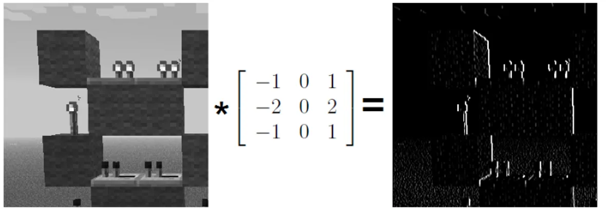
Figure 2.2: Grayscale image convoluted with a horizontal Sobel Kernel to produce an image with highlighted edges

The first step is to create the two different Sobel edge finder images in horizontal and vertical orientation to obtain the intensity change in both directions (Fig. 2.2). The edges of an image play a vital role when locating corners since corners could essentially be defined as junction of edges. These two images are then combined into three new compound images, which are used to find eigenvalues. In a final equation a single value is produced that can be thresholded to separate data points indicating an edge, corner or flat area. A post-filter is often utilized to suppress positive data points nearby a local maximum value, giving the final image a collection of single pixel dots on each corner response.

(15)

Due to its popularity, the Harris corner detector exists as a function in OpenCV.

2.4 FPGA

Invented back in the 1980’s by Ross H. Freeman, an FPGA-chip is comprised of repro-grammable hardware [9]. Conventional microchips and Central Processing Units (CPUs) are static and their internal structure cannot be changed. They are specifically manufac-tured to process software as efficient and fast as possible, but always one single instruction at a time. AnFPGAon the other hand, contains many Configurable Logic Blocks (CLBs) that can be connected to each other in different ways as defined by a HDL. This gives the freedom to process many input data in parallel with the possibility of speeding up computation time by orders of magnitude. If the architecture is faulty or outdated, it can simply be reprogrammed, while a static chip such as an Application-Specific Integrated Circuit (ASIC) would have to be replaced completely.

Resource Type Description

Flip-Flop (FF) A small element of gates able to store one data bit between cycles Look-Up Table (LUT) An N-bit table of pre-defined

responses for each unique set of inputs Digital Signal Processor (DSP) A block with built-in computational

units such as adder, subtracter and multiplier Block RAM (BRAM) A block of dual port RAM memory

very close to the FPGA fabric

Table 2.1: Some of the logical block types in the FPGA

The internals of an FPGA are made up of many instances of a couple of logic units such as multiplexers, Flip-Flops (FFs), Look-Up Tables (LUTs), and memory blocks called BRAM. There are also Digital Signal Processors (DSPs), often in the hundreds, that can assist in floating point operations. The HDL provides a way for the user to specify the behaviour of the system. The code is then used to synthesize an actual digital circuit that is implemented for the FPGA hardware to determine which of its resources are connected to which.

2.5 Zynq 7000

The Zynq 7000 SoC from Xilinx is a series of chips with both a FPGA and CPU built in to the same chip, allowing very fast interaction when accelerating programs. With support for DDR3 speed memory interface, it allows the FPGA and CPU to also share external memory usually much bigger than the available internal memory.

All chips of the 7000 series use a Dual ARM Cortex-A9 as CPU. The main difference between different chips in the series is the FPGA specifications that range from 28K Logic Cells, 17,600 Look-Up Tables (LUTs), 35,200 Flip-Flops and 80 Digital Signal Processors (DSPs) on the lower end, up to 444K Logic Cells, 277,400 Look-Up Tables (LUTs), 554,800 Flip-Flops and 2020 Digital Signal Processors (DSPs) on the higher end. [10]

The chip used in this thesis is called Zynq 7020 (XC7Z020) and is equivalent to the Artix-7 FPGA. Its resources are in the low-end range of the product table with 85K

(16)

Logic Cells, 53,200 Look-Up Tables (LUTs), 106,400 Flip-Flops and 220 Digital Signal Processors (DSPs) with 560KB Extensible Block RAM. [11]

2.6 GIMME-2

The GIMME-2 is a second generation stereo vision system, designed to replace GIMME [12] (General Image Multiview Manipulation Engine). It is equipped with a modern Zynq-7020 FPGA chip and two high resolution camera chips spaced approximately the same distance as between human eyes. [13]

Some of its key features are: • 1x microSD

• 1x Fast Ethernet • 2x Gigabit Ethernet

• 2x 10 MegaPixel CMOS Camera Aptina MT9J003 • 3x DDR3 4Gb Devices

• 3x USB2.0

• Zynq 7020 SoC with ARM Cortex-A9 Dual-Core CPU

While this thesis was somewhat aimed for the GIMME-2 platform, no real testing was performed on that, but instead on the ZC702 Evaluation Board equipped with the same Zync SoC chip. [1].

(a) (b)

Figure 2.3: (a) Back side of GIMME. Note the image sensors on the right and left side of the top part. (b) Front side of GIMME2.

(17)

2.7 High-Level Synthesis

The basic idea of any HLSTis the same as many other programming languages; abstrac-tion. In the same way assembler streamlined programming when it replaced machine code, and languages such as C applied further abstraction when in turn replacing assembler. Programming C/C++ often represents the brains way of thinking rather sequentially about an algorithm better than what a Hardware Description Languages (HDLs) repre-sents. The benefits are even more apparent the bigger the system to be designed is.

In a classic C program it is rather straightforward what a piece of code does, and in which order the program will run, while still being abstract enough so the user does not have to worry about exactly what the CPU will do. Hardware Description Languages (HDLs) are also a type of abstraction, but the user still has to constantly keep in mind what runs in parallel. With big systems it can be hard to keep track on what happens at the same time as what.

High-Level Synthesis Tools (HLSTs) also makes system designs easier to modify and/or repair. Most of the time it is rather trivial to add/remove some code in a C/C++ program, compared to changing something in the core of a HDL design. Another strength is how the performance gain can be tweaked to perfectly match a timing constraint. If an image processing solution is designed to run at 30 FPS and is fed images at that rate, it would be a waste to use 50% of the FPGA’s available resource to make it capable of running at 120 FPS, if it instead could be tweaked to use only 20% resources running at 35 FPS. [14].

2.7.1 History

The roots of HLScan be tracked all the way back to the 1970’s, but the work done back then was mainly research. It was not until the 80’s and primarily 90’s it started gaining commercial success [15]. It still did not break through however, and part of the reasons why was that the High-Level Synthesis Tools (HLSTs) of those days were aimed at users already very familiar with RTL synthesis, who did not really find a use for the tools unless they presented significant design time reduction in addition to similar or better quality results. This was not the case though as ”In general, HLS results were often widely variable and unpredictable, with poorly understood control factors. Learning to get good results out of the tools seemed a poor investment of designers’ time.” [15]. The sales of High-Level Synthesis Tools (HLSTs) saw an almost all-time low in the early 2000s and stayed like that for a few years until the next generation.

When generation 3 of High-Level Synthesis Tools (HLSTs) came along, the sales had a rapid increase around 2004 and a big difference this time was that most High-Level Synthesis Tools (HLSTs) started targeting languages such as C and MATLAB. Users needed no previous HDL experience to utilise these tools and could focus on what they already did best; algorithm and system design. Also, the quality of results had also improved a lot, boosting success even further. Today is still seeing that success and development is still going strong, leading to a multitude of different design tools available on the market.

(18)

2.7.2 Toolsets on the market

There are currently many different C-to-HDL compilers on the market. Some of them are Catapult-C2, BlueSpec3, Synphony4, Cynthesizer5, and the product that this thesis mainly focuses on: Vivado HLS6 _{earlier known as AutoPilot before Xilinx acquired it}

from AutoESL in early 20117_.

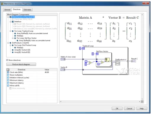
LabVIEW, from National Instruments, utilizes HLS in their FPGA IP Builder. This is an interesting tool because the input algorithms are not produced with written code, but with LabVIEW’s drag and drop GUI. The Virtual Instruments (VIs) is also optimized through a GUI that adds directives which will be explained in Subsection 2.7.5Pragmas, Code Optimization and Synthesizability. A hardware designer using this system would never touch the code, only windows and interfaces [16].

Figure 2.4: An algorithm represented by a VIcreated in LabVIEW, ready for optimiza-tions with directives. All done through a GUI

2.7.3 Designing with Vivado HLS

Design Philosophy When writing the C/C++ program to be synthesized, the design philosophy of Xilinx is that there should not initially be too much thought put into that fact. The more constraints and hard coded limitations that are put in the code in an attempt to manually optimize it while still designing it, the more it could limit design variations for the HLSTcompiler to ultimately experiment with.

This initial code process can advantageously be done completely within a function since the code to be accelerated can be thought of as a single function called from a program.

2_{http://www.calypto.com} 3_{http://www.bluespec.com/products} 4_{http://www.synopsys.com} 5_{http://www.forteds.com} 6_{http://www.xilinx.com/products/design-tools/vivado/integration/esl-design/index.htm} 7_{http://tinyurl.com/Xilinx-acquires-AutoESL}

(19)

In fact, when later preparing the C/C++ code for acceleration, Vivado HLS wants a top function to be defined by the user, and it is this function that will be accelerated. The inputs and outputs of that function is then the interface between the PS, and the FPGA/PL.

The finished accelerator (Also called Intellectual Property (IP)-Block) can not be called from a C/C++ program in the same way that a normal C/C++ function would. However, it can and should be used in a test bench to confirm it works as intended before the C/C++ code is synthesized to that accelerator. The initial code created before Vivado HLS can then be used as reference in that test bench.

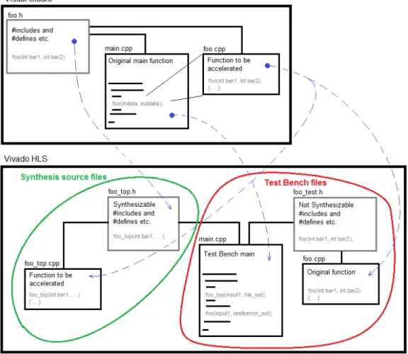
Managing the code files in Vivado HLS can be tricky since everything that can be synthesized has to be separated from that which can not, but all files in the project for the C simulation (Fig. 2.5).

This design phase for starting a new Vivado HLS project can be split up in to key steps

1 Write a C/C++ program (in Visual Studio for example). Put all algorithm code in a single function to easier separate the overhead code (like loading images or similar) from the actual algorithm to be accelerated. Use a .h file for includes and function declaration.

2 In Vivado HLS create two Test Bench .cpp files, one with the function from step 1, and one with the main() from step 1. Any other utility files or similar can also be put in as Test Bench files, since they will only be used during C Simulation.

3 Create a new Source .cpp file. Put only the function to be accelerated from step 1 here. Vivado HLS will try synthesize all files listed as source in this project.

4 Name this function something other than its Test Bench variant. Then in Project Settings → Synthesis, put that exact same name in the Top Function field.

5 Use the same .h file from step 1 as a ”top include file” that spans both the Source and Test Bench. Declare the header of the Top Function from step 4 here since it will be used by the Test Bench for verification. Add this .h file to the Source files since it will be used in synthesis.

6 Create a second .h file, this time in the Test Bench. This header file will only be included in the Test Bench source files, and thus can contain any unsynthesizable functions/includes needed for validation during C simulation (OpenCV libraries for example).

7 In the Test Bench main(), include both .h files from step 5 and 6. Call both the Top Function from step 4, and the test bench function from step 2 and use the exact same input data. (they should still be identical in this step, except for their names). 8 Add some code that compares the output data from both functions and exits with

0 for success, and 1 for failure..

9 Test run the Test Bench. It should now run the two functions with same input data and compare their output which should be identical.

(20)

Figure 2.5: Initial process for starting a Vivado HLS project. Note that while Test Bench files only spans the three right ones, all five files are actually part of the C Simulation. The parts of foo.h that is not synthesizable, but needed in the test bench, are moved to foo test.h

2.7.4 Test Bench

The Test Bench of Vivado HLS is one of the great advantages over HDL coding. In fact, Xilinx states that not using a Test Bench before synthesizing the code is ”The single biggest mistake made by users new to a Vivado HLS design flow” [17]. Since the code to be synthesized will always be written in C/C++, it is relatively easy compare its functionality with the C/C++ code it originated from.

The test bench looks like a C/C++ program with a main() function. The idea is to run both the Top Function that is to be synthesized, and the C/C++ code that it intends to mimic, compare their results and finally return with a message saying if it passed or not.

It’s important to note that Vivado HLS will attempt to synthesize the ”top include file”, since it must be included in .cpp file with the Top Function. It will run just fine during C Simulation, but will cause an error is synthesis is started with unsynthesizable code in it (such as OpenCV libraries). Any parts of the top include file that is not synthesizable, but is still needed for the test bench, must therefore be moved to a separate .h file that only spans the Test Bench by including it only in test bench files (covered in

(21)

step 6).

Vivado HLS can also run a C/RTL Co-simulation using the synthesizedRTLwith the test bench. With a finished and working test bench, and synthesized RTL, Co-Simulation is just a click away. This will test the synthesized RTL by first using the test bench to generate input for the RTL, and then run it through the RTL. Finally, the results of the RTL simulation is used in a new run-through of the C/C++ test bench. If successful, a latency report is generated and, if selected, a waveform report for more detailed study.

2.7.5 Pragmas, Code Optimization and Synthesizability

When the C/C++ code has been imported as a Top Function and is confirmed working, it is time to prepare the code for HLS. The performance gain of converting a C/C++ program to HDL that runs on an FPGA comes from the HLST focusing on several key features such as:

• Flattening loops and data structures such as arrays and structs, for better paral-lelism and less overhead

• Unrolling loops, executing several - or all - iterations simultaneously • Merging loops for lower latency and overhead

• Pipelining loops and functions to increase efficiency

How much the code should be affected by such a feature, and which parts code to affect is determined by directives. They also define which type of interface the hardware accel-erated function should have with the PS, as it could otherwise produce a bottleneck for the accelerator if a low bandwidth option is chosen.

This process of preparation is mainly done by ”tagging” blocks of code with these directive, which instructs the compiler how to synthesize that block of code to HDL. The directive are usually specified using pragmas.

In conventional C/C++ programming, pragmas are a way to instruct the compiler something. A common usage is #pragma once put at the top of a header file to instruct the compiler only to include that header file once [18]. Vivado HLS aims to streamline the directive placing process by providing users with GUI options to insert such pragmas at key locations in the code.

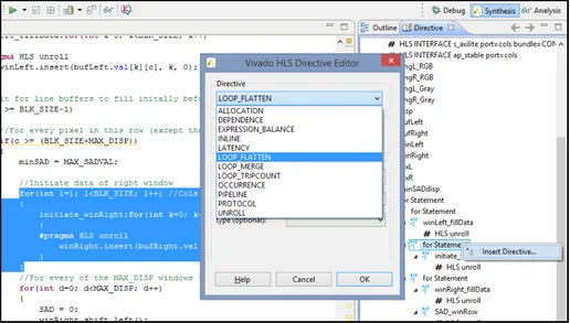
When the Top Function is to be prepared for HLS, there is a ”Directives” tab in the GUI that lists items named ”for Statement” or ”while Statement” etc. that represent different blocks of code in the C/C++ program. A block of code here means the code in the scope, i.e. the code between a bracket ”{” and its corresponding closing bracket ”}”, such as loops and functions and so on. The user can then right-click on a specific item in the list - highlighting the corresponding scope in the code - and click ”Insert Directive...” and in a list select between a variety of available directives (Fig. 2.6). The HLST will then automatically insert a line of code (usually a pragma) at the start of the selected item’s scope in the source file. This will alter the synthesized behaviour of the block of code. There is also the option to instead place the directive in a directives.tcl file, which has the same effect, but avoids littering the C/C++ code with pragmas.

(22)

Figure 2.6: Vivado HLS Directive GUI. The list to the right shows they key parts of the code, such as for loops or the variables of the function header. Right clicking gives the option to add a directive there in a popup window [17].

Loop Unrolling Unrolling a loop will result in multiple iterations executing simulta-neously. It can be partly unrolled, meaning the whole loop is completed in bunches of N, where N is a number specified by the user. N = 3 indicates three iterations of the loop completed simultaneously, and then the next three are done simultaneously etc. A fully unrolled loop is when N = max loop iterations, resulting in all iterations of the loop executing in a single clock cycle.

The default setting in Vivado HLS is to leave loops unchanged (rolled). This is because unrolling a loop is directly related to how much resources of the FPGA is used. Running an unrolled loop where N = 2 means double the speed, but also double the resource cost. As one can imagine, a fully unrolled loop can claim a sizeable chunk of resources if it is big (Fig. 2.7).

If an iteration of a loop is dependant on the result of an earlier iteration, loop unrolling is not possible. [17, p 145]

This directive is reminiscent of how loops work in VHDL where all iterations of a loop are indeed executed in a single clock cycle.

Loop Merging When multiple loops are executed in sequence there may be an op-portunity for loop merging. This essentially means that instead of running each loop separately, the contents of both loops can be merged in to a single loop. Thus the amount of states the final hardware has to run through is reduced, while still using the same amount of resources. This is because there is always an overhead of one cycle to enter a loop, and one cycle to exit a loop, and each loop’s iterations are executed separately from other loops’, even though they do not use the same resources. Putting the contents of both loops in to a single loop not only eliminates the extra cycles for entering and exiting the loop, but more importantly executes contents of both loops simultaneously.

Loop merging requires the loops to have constant bound limits - where the highest constant will be used in the merged loop - or if variable limits, it must be the same variable in both loops. There must also not be any dependencies between the loop contents. As a rule of thumb, multiple executions of the code must generate the same result. [17, p 149]

(23)

Figure 2.7: Three different synthesized examples of the same loop defined by the C code in the grey box. Rolled Loop results in 4 clock cycles, but few resources used while the unrolled examples use more resources for 2 and 1 clock cycle execution respectively [17].

Loop Flattening In loop merging the latency cost of entering and exiting a loop was mentioned; it takes the FPGA one cycle to enter a loop, and one cycle to exit a loop. It may not be that big of a latency difference when merging two separate loops, but when the loops are nested it bears a much bigger significance. Imagine an outer loop running for 100 iterations, with an inner loop running 5 iterations. This would cause a total of 200 cycles spent on entering and exiting the inner loop. Loop flattening helps this issue by removing the inner loop, and moving the loop body to the outer loop, significantly reducing loop execution overhead. [17, p 151]

Pipelining There are two types of pipelining: Loop Pipelining and Loop Dataflow Pipelining. The former is applied on a single loop to pipeline its contents, while the latter can pipeline a series of loops or functions.

Loop pipelining is applied on a loop to allow each part of the loop to execute all its iterations in parallel to the other parts. For example, if each iteration of a loop contains three operations: one read, one computation, and one write, it can be pipelined to read on every clock cycle instead of every third (Fig. 2.8). Thus, a new loop iteration is begun on every clock cycle, before the previous iteration is done. A constraint for using pipelining is that the execution of an iteration must not depend on the result of previous iteration(s) since it then would have to wait for all previous iterations to complete.

Loop Dataflow Pipelining operates on a bigger scope. It will pipeline multiple separate loops to execute their iterations independently from the other loops. This directive also works for series of functions in the same way. The biggest constraint is that the variables must be produced by one loop/function and consumed by only one other loop/function (Fig. 2.9).

This directive is often used in this thesis as the code is often consisted of several image filter functions operating on the same image stream.

(24)

Figure 2.8: The loop contents are pipelined so that a new iteration can begin before the previous one is completed [17].

Loop Carry Dependencies In some scenarios data is read and written to the same array, but the developer knows it’s never to the same parts of the array. For example, a loop uses data from the first half of the array to calculate values to save in the second half. This can be hard for Vivado HLS to recognize, so any loop containing such an access pattern will be synthesized fully sequential. This can be overridden by using a dependency directive

2.8 C Libraries for HLS

Xilinx realised that OpenCV is a very useful library for HLSsince it presents easy to use, and well known image processing functions in C/C++. The problem with OpenCV is how the images are stored during runtime. As briefly described in Section 2.1 OpenCV, the memory is used dynamically, and that does not translate well to an FPGA, since it does not have that type of access to that size of memory (More details in next Subsection 2.8.1 Memory Management ). Instead the images are interpreted as streams of data.

Moreover, each image filter has its own characteristics and they can all be optimized in different ways, so instead of only translating the Mat structure to HLS friendly code, Xilinx have also translated many individual image filters, and therefore constructed a imaging processing library of their own, with derivatives of OpenCV’s most popular functions.

The library is named hls_video.h and the functions in it are tailored for HLS and optimized for hardware [19]. They still work as normal C/C++ functions, but ”The library functions are also intended to be compatible with existing OpenCV functions and are similarly named, however they are not direct replacements of existing OpenCV” (Xilinx UG902 [17]).

Xilinx has also created a HLS-friendly version of hls_math.h from C/C++ as it is likely frequently used in any software that would require hardware acceleration. This aids particularly in HLS for functions with floating point operations.

(25)

Figure 2.9: The separate loops are pipelined so that each consecutive loop can execute its iterations independently [17].

2.8.1 Memory Management

As mentioned, FPGAs do not use memory in the same way as a normal CPU. While GIMME-2 and the ZC702 Evaluation Board both have Gigabytes of external RAM mem-ory, this memory can only be accessed through a dedicated Direct Memory Access (DMA) block, which can address and read/write data from/to that memory. Since FPGAs are highly parallel systems, continuously accessing external RAM for every temporary vari-able storage, or every sliding window buffer, will most likely bottleneck the system due to the external memory’s few data channels. Instead the FPGA comes with programmable Block RAM inside the fabric, usable for buffering data during calculations. This memory is very limited in size however, and as stated in Section 2.5Zynq 7000, the ZC702 Evalu-ation Board used in this thesis has 560KB Extensible Block RAM, in chunks 36Kbit per block (140 blocks). Each block has a true dual-port interface where read/write ports are completely independent and share nothing but the stored data [10].

The hls::Mat class represents the cv::Mat class with the big difference that the HLS version is defined as a data stream (hls::stream) since an image of any respectable size would exceed the 560KB internal memory. The finished IP-block would instead expect a steady stream of pixel data, one pixel at a time, which a big external DDR3 RAM memory is ideal for.

However, since most image filters need to use the data of a pixel several times, such as stereo vision requiring a sliding window of N×N pixels, Xilinx has provided two very similar data structures for this purpose. hls::Window and hls::LineBuffer. In C/C++ code, these classes are defined as your typical 2-dimensional array of whichever data type is used. Note that only the data storage declaration and directives are kept in the following

(26)

code snippets, while other functions has been removed for de-clutter reasons. Line Buffer

template<int ROWS, int COLS, typename T> class LineBuffer {

public:

LineBuffer() {

#pragma HLS ARRAY_PARTITION variable=val dim=1 complete };

T val[ROWS][COLS]; };

First of all, this class is capable of storing different data types due to its template structure. Secondly, the ARRAY_PARTITION pragma will mark the array’s first dimension (rows) to be completely partitioned in to block RAM during synthesis. Now the data of each row can be accessed independently of the other rows. The class also comes with functions to shift data up/down and assumes that new data is input in the resulting ”empty” using the insert function.

These functions are defined so that the LineBuffer data is indexed 0 in its bottom-left position. Therefore shifting down means the actual data is actually moved up, because the LineBuffer structure is thought of as a window with the same width as the image, and sliding down over the image, resulting in the data moving up inside that window. It’s intended to be used with few rows, but is flexible on amount of columns.

Window The hls::Window is very similar with some key differences. template<int ROWS, int COLS, typename T>

class Window { public:

Window() {

#pragma HLS ARRAY_PARTITION variable=val dim=1 complete #pragma HLS ARRAY_PARTITION variable=val dim=2 complete

};

T val[ROWS][COLS]; };

The window is completely partitioned in both vertical and horizontal dimensions for a fully parallel memory access, so each element in the window can be accessed individually. Moreover, the Window class also have data shift functions for left/right on top of the up/down found in LineBuffer. In the same way as the LineBuffer, the Window can be visualized as an actual Window sliding over the data, resulting in the data indexed not just from bottom-up, but now also from right-left. The index origin therefore is now in the bottom-right position. Due to its complete partitioning, this data structure is intended to be used with rather few rows as well as columns. As a result of the complete array partitioning and the fully parallel element accessing, a Window is usually synthesized with Flip-Flops as a sort of shift register instead of using Block RAMs (BRAMs). Thus, the developer’s Window sizes are effectively limited by the available Flip-Flops [20].

(27)

Chapter 3 Related Work

There have already been experiments conducted with High-Level Synthesis Tools (HLSTs) in different fields of research, both with Vivado HLS, and other tools. Here follows a couple of the most relevant works.

3.1 Optical Flow HLS

An optical flow algorithm detects the movement of key features in a series of images by comparing two consecutive frames. In 2013, Monson, J. et al. used Vivado HLS to implement such an algorithm for the Zynq-7000 [21]. The algorithm was tested on both the ARM Cortex A9 processor and the FPGA in the Zynq-7020 chip (same chip used in this thesis), and was compared with the results from an Intel Core i7 860 2.8 GHz [22] desktop running Windows 7.

Design The previous and next images were first processed to an image pyramid which is a set of the same image with different resolution. In the bottom of the pyramid is the image with highest resolution. Each step up is a result of downsampling with a Gaussian smoothing filter and removal of odd rows and columns. Each level of the pyramids is then processed through a gradient filter with a Scharr kernel to produce both a horizontal and vertical gradient pyramid (Fig. 3.1). These images are then used in a similar fashion as in Harris Corner Detector to find interest points, which are the points tracked between images.

The design was fed images of 720×480 and used 15×15 integration windows, tracking between 350-400 features.

In their work, they split the design in to three major parts: The pyramid creation, the Scharr filtering, and the feature tracker. The performance of the pyramid creation and Scharr filtering parts do not change depending on what’s in the image, only its size, so they were simply given an estimated speed-up of 3.9× and 5.6× respectively, if implemented with FPGA. The feature tracking part was harder to estimate, and since it took up 67.3% of the execution time on the ARM, it was the only part put through the Vivado HLS process to get a more accurate value.

Vivado HLS Process The first iteration of HLS kept the original code structure as much as possible, only removing the parts with dynamic memory allocation and any recursive functions etc.

(28)

Figure 3.1: Grayscale image convoluted with a horizontal Scharr Kernel to produce an image with highlighted edges

To optimize the design, the dataflow directive was applied to make use of the parallel nature of FPGAs. To better achieve this, the code was restructured by splitting up the main loop in two different parts, representing two sub-parts of the feature tracker.

Version LUTS FF DSPs BRAMs Latency (cycles) Clock Rate baseline 22,647 (42.6%) 16,171 (15.2%) 110 (50.0%) 23 (8.2%) 5,171,563 95 MHz dataflow 34,007 (63.9%) 32,844 (30.9%) 196 (89.1%) 201 (71.7%) 2,590,972 100 MHz

scharr 37,266 (70.0%) 33,601 (31.6%) 194 (88.2%) 185 (66.1%) 2,518,141 100 MHz max. clock 37,055 (69.7%) 33,626 (31.6%) 194 (88.2%) 185 (66.1%) 2,538,290 110 MHz

Table 3.1: Resource usage of the Optical Flow algorithm. [21] Copyright c 2013, IEEE

Results On the i7 desktop system all 4 CPU cores could be used to achieve 80-90 FPS. On the ARM Cortex-A9 only 1 core was utilized for a 10-11 FPS result. Finally, the FPGA solution achieved 41.8 FPS. Interesting also is the power usage where the FPGA solution used 3.2× less energy than the ARM, and 7.4× less than the i7. While the FPGA achieved about half the speed of the i7, 41.8 FPS is still a good real-time result.

It is worth taking a look at the resources used for this implementation. Looking at Table 3.1 it can be seen that the solution used 88% of available Digital Signal Processors (DSPs), 70% of Look-Up Tables (LUTs) and 66% of Block RAMs (BRAMs). The baseline design, where minimal amount of code altering was applied, used significantly less, but only achieved 18.4 FPS.

3.2 Stereo Vision HLS

In [23] (2011) an older version of Vivado HLS (then named AutoPilot) was used to test five different stereo matching algorithms on a Xilinx Virtex 6 LX240T (with 3-4 times more resources than the Zynq-7020).

Design In this work, Five different stereo vision algorithms were tested. • Constant Space Belief Propagation (CSBP)

• Bilateral Filtering with Adaptive Support Function (BFAS) • Scanline Optimization with occlusion (SO)

(29)

• Scanline Optimization without occlusion (SO w/o Occ) • Cross-based Local Matching (CLM)

None of their source codes were made with future HLS in mind. They were rather optimized for software execution. This design was created before Xilinx had created the HLS video library, so any part of the code using OpenCV had to be remade.

Vivado HLS Process The code preparation for HLS was divided up in distinct steps and evaluated after each step.

Just as in the Optical Flow paper, this paper describes a baseline design with only the bare necessities for the code to be synthesized.

After that first step, directives and code restructuring was used to start optimizing the design.When it comes to image filtering algorithms in general, the most important such restructuring would be to divide the image in to different parts, and to operate on all parts simultaneously. More specifically; stereo vision is often inherently row-centralised, so each row can more or less be processed individually. The only algorithm that was fully inter-row independent was SO. The other algorithms applied a windowing solution, such as the one described in Section 2.2 Stereo Vision, which would access several nearby rows at once. An image can still be divided into sub-images though, as long as the edges overlap somewhat, to allow windows accessing data outside the sub-image.

The third step was reducing bit-width and memory usage by specifying variable pre-cision and merging arrays to use fewer Block RAMs (BRAMs).

The fourth step saw loop optimizations applied and pipelining employed. This also required some restructuring of the code, and often an upper loop bound had to be set since variable length loops does not translate well to hardware. With static loop bounds, it is much easier for Vivado HLS to flatten, unroll or pipeline the code.

Finally, any remaining unused resources after step four can be used to parallelise by resource duplication. Essentially computation pipelines are duplicated to hopefully dou-ble the speed. This step was not as easy as inserting a directive since Vivado HLS (then AutoPilot) did not have a directive to simply parallelize the code. It was more a question of the synthesizer recognizing which parts of the computation are independent from each other. They achieved this using a trick essentially identical to partial array partitioning and loop unrolling. They would expand some arrays with a new dimension defined as FS_UNROLL, which was set as 2 in their example, making the array 2 times as big. Those arrays were then used in a nested loop, where the outer loop would iterate in steps of FS_UNROLL and the inner loop - the one that would access the data in the arrays - would loop only FS_UNROLL times. Only the inner loop was completely unrolled, essentially telling the synthesizer that every instance of the new dimension could be accessed inde-pendently of the others. For even greater parallelization, FS_UNROLL could of course be increased.

Results The initial baseline code transformation synthesized into extreme resource us-age, and only the SO algorithm would actually fit on the FPGA, but this was not too surprising since no optimizations had been applied at all. The next step (code restructur-ing) would drastically decrease resource usage. Every step after would then successively decrease resource usage, while increasing performance. Performance did not increase by any great amounts until the last step, the parallelization, where algorithms received between 3.5× and 67.9× speed-up over the software version, and also vastly increasing

(30)

Figure 3.2: Resource use (left y-axis) and speedup (right y-axis) for every stage of each of the five different stereo vision algorithms. Figure from [23]. Copyright c 2011, IEEE

resource usage (Software execution was performed on an Intel i5 2.67 GHz CPU with 3GB of RAM. Likely the 2009 Intel i5-750 [24], but it is not exactly specified in their paper). Looking at Fig. 3.2, it can be seen that the SO w/o Occ algorithm achieved the highest speed-up while the other algorithms were under 20×.

Algorithm Development Effort

BFAS 5 Weeks

CSBP 3 Weeks

CLM 4 Weeks

SO 2.5 Weeks

Table 3.2: Development effort for each algorithm in Vivado HLS, normalized to the development time of a single hardware designer. [23] Copyright c 2011, IEEE

They compare these HLS designs with pure hardware designed solutions, for example a manual hardware implementation of the CLM algorithm saw a 400× speed-up but ”required 4-5 months of design effort for an experienced hardware designer to implement the design, plus additional time for a team to design the algorithm.” [23]. At the same time, they acknowledge that ”although AutoPilot has powerful optimizations available, it is sometimes difficult to apply it to code that was not designed in advance to use the optimization.”.

The development effort for their results are summarized per algorithm in Table 3.2. Note that the time has been normalized to represent the time spent by a single hardware designer.

(31)

3.2.1 Other Related Work

In [25] (2013), J. Hiraiwa and H. Amano compares manually written Verilog HDL to Vivado HLS synthesized code in a pipelined real-time video processing architecture. While the manually coded HDL took approximately 15 days to complete, the Vivado HLS code took only 3 days, and the resulting latency of both implementations showed no significant difference. This came at the cost of about 3-4 times higher FPGA resource usage.

An example of the performance impact of different magnitudes of loop unrolling can be seen in [14] (2013), where ¨Ozg¨ul, B. et al. compare three different Digital Pre-Distortion (DPD) solutions, each with different complexity. Each solution is also tested in four different variants:

1 A software program only

2 The same software program, but with the main loop hardware accelerated

3 The same software program, but with the main loop hardware accelerated and unrolled by two

4 The same software program, but with the main loop hardware accelerated and unrolled by four

The programs were synthesized with Vivado HLS, and tested on Xilinx ZC702 develop-ment board. The results presented a speed-up of between 7,7-10,4× over the software program when compared to the four times unrolled hardware accelerated main loop. The total latency in those cases showed close to 5 times lower across the board.

As expected, the speed-up was less apparent when unrolled by two, or not at all, but those solutions of course resulted in less FPGA area used. This is a good example of how the performance can be tweaked perfectly to a certain timing constraint. The DPD had a timing constraint of 300 ms, and these results made it possible to sometimes choose the solution unrolled only twice, or the one not unrolled at all but still hardware accelerated, to use as little resources as possible and still meet the constraint.

In [26] (2013) HLS is used to develop digital control of power converters showing significant design complexity reduction.

(32)

Chapter 4 Method

4.1 Xilinx Toolchain

While the main focus of the Thesis was to evaluate Xilinx’s HLST, other tools of the Vivado toolchain were also used in order to realise the project. The component generated in Vivado HLS would typically be added to a design created in another program, called Vivado, in order to properly interface it with the PS and grant memory access. After synthesis and implementation of the design in Vivado, a bit-file is created to program the targeted FPGA. Finally, in order to control the FPGA behaviour from the PS, the hardware specification is exported from Vivado to Xilinx Software Development Kit (SDK) where drivers can be implemented in C code to interface Linux or a standalone OS -with the hardware inside the FPGA.

4.1.1 Vivado

Vivado is a new design program from Xilinx first released 2012 that intends to replace their old ISE design suite, which is no longer updated as of October 20131_{. The functionality of}

ISE design suite programs such as the Xilinx Platform Studio (XPS), ChipScope waveform analyzer and PlanAhead IP Integrator, are now all part of this new Vivado tool. It is used to create the whole design of the RTLcomponents to be synthesized and implemented on the chip. Note that this is not the same program as their HLST which is called Vivado HLS.

Since Vivado design suite was new, the ISE design suite was also installed as parts of it had yet to me migrated such as ChipScope.

IP Blocks Vivado allows a user to create a design without forcing them to work with individual VHDL/Verilog code files, but instead uses completeIP Blocks that appears as boxes with pins for inputs and outputs used in a drag and drop fashion in the IP Integrator feature. This gives a good overview of the whole design and at the same time lets the user connect signals, buses and clocks without writing any code (Fig 4.1). Most IP blocks can also be customised to some extent through a GUI accessed by double clicking the IP block in the IP Integrator. Depending on the IP there are different settings available, such as bit width of AXI4 stream, number of slave and/or master connections, color mode (i.e. YUV or RGB style etc.), timing mode and FIFO buffer depth to name a few (Fig 4.2).

(33)

Figure 4.1: Vivado IP Integrator with several IP-Blocks.

A component generated in Vivado HLS would typically be one of those IP-Blocks. Vivado also comes with a library of a number of IP-Blocks from Xilinx ready to use, such as the Video Direct Memory Access (VDMA), Test Pattern Generator (TPG), and the essentialPSIP used to interface any FPGA design with thePSof the Zynq. It is through the PS IP that the VDMA IPs access the external DDR memory using up to four High Performance (HP) ports. It is also where the clocks and other I/O are defined.

PS/PL Interface Many IP Blocks can communicate with thePS, as well as each other, through a bus interface called Advanced eXtensible Interface (AXI), which comes from the ARM AMBA protocol [27]. AXI communication can be done in three different ways. An IP Block’s behaviour and general settings are often controlled through an AXI4-Lite bus, as it is suited for low-throughput memory-mapped data transfers (i.e. reading/writing

(34)

Figure 4.3: The Address Editor, where each IP gets an address space defined for AXI communication.

status registers). Sending and/or receiving bigger data, such as an image, is often done through a standard AXI4 interface, which is more suited for high-performance memory-mapped operations. The third interface is AXI4-Stream which is used to continuously send a lot of data in high speed, for example streaming video. [28]

Address space All the IP Blocks with an AXI4-Lite interface utilise the shared memory between thePSandPLto communicate. This means each such IP Block needs an address space which is assigned in Vivado before synthesis (fig 4.3). Standard AXI4 bus data transfer is usually done through some sort ofDMAwhich then feeds the consumer blocks. In this thesis, mainly the VDMA was used as it is specialized for sending streams of images. Control buses through AXI4-Lite normally gets a small 64 kB space for simple register I/O, while the AXI4 and AXI4-Stream interface can go up to gigabyte levels if needed. This address space can then be used from programs running on the PS to configure IP settings, or transfer images/data from/to the PL.

When the bitstream is finally generated after synthesis and implementation, Vivado can export a hardware specification file containing all addresses used in the design. This specification can then be imported and used in the SDK.

4.1.2 SDK

The XilinxSDKis used to write C/C++ drivers and programs to control the behaviour of the FPGA. The hardware specification imported from Vivado is used to make a hardware platform project used to initiate the board. A Board Support Package (BSP) can then be created if Xilinx’s standalone Operating System (OS) is used, containing drivers to devices on the board such as I2C and USB etc. Finally, a user can create their custom Application Project for their purposes. In this thesis, Linux was used as OS Platform, thus limiting the use of the BSP to mainly retrieving the AXI4 interface addresses.

The SDK compiles the Application Project to .elf files which is then executed on the ARM processor in the Zynq.

Linux The AXI4 interfaces have a physical memory address space assigned to them. To use this in linux, it must first be mapped to its virtual memory space. This is done through the mmap() function. The memory can then be written to and read from, usually through volatile pointers. This is used to control the FPGA design.

(35)

4.1.3 Tcl

Most of Xilinx’s programs are based on the Tool Command Language (TCL) script lan-guage. Both Vivado and Vivado HLS have the option to launch in command mode, skipping the whole IDE for a lightweight console interface. This can be especially useful when sharing a project, or when a whole project design using the whole Vivado toolchain is to be generated with one script, or just store it without wasting hard drive space.

For example, a Vivado HLS project’s source files can be bundled with a simple run-Script.tcl script file that - when run through the Vivado HLS Command prompt with vivado_hls runScript.tcl - will set up the project folder hierarchy and add appro-priate files as Test Bench or Source files respectively. This folder could then be opened through the Vivado HLS GUI for easier navigation and editing, or the runScript.tcl could be written to run C Simulation, Synthesis, Co-Simulation and IP-packaging all in one go.

This was utilized when asking for advice on the Xilinx Forums as a quick way to share the code.

(36)

4.2 Intro Project

To get familiar with the toolchain, a number of demo projects are available, called Xilinx Application Notes. The Application Notes are named xapp followed by a number.

xapp1167 was particularly relevant as it was a demo of a Vivado HLS synthesized IP block [29]. The block was used in a design to compare OpenCV functions executed on the PS, with their acceleratedHDLversions running on thePL. The xapp comes with all files needed to build a boot image for linux, synthesize an example image filter in Vivado HLS, generate a bitstream with a design that uses the image filter, and build the .elf -file to run on the PS to interface with the PL. The xapp did not use the Vivado toolchain, but the now deprecated ISE design suite.

After a simple make all command everything compiled and was ready to run on the ZC702 Evaluation Board. It is rather quick to get it up and running and see the obvious differences of running an OpenCV image filter on thePScompared to the FPGA accelerated image filter. The PS had a very low and choppy framerate while the image filter on FPGA was constantly high FPS and smoother.

The input image data was generated from a Test Pattern Generator (TPG), an IP block that comes with Vivado. A TPG can be setup, either directly before synthesis or later through the PS, to generate patterns at different sized and colors.

The demo image filter comprised of a chain of 5 OpenCV filters with no real practi-cal use other than to show performance difference. (Note that this example does not use the C++ version of OpenCV)

cvSobel(src, dst, 1, 0);

cvSubS(dst, cvScalar(50,50,50), src); cvScale(src, dst, 2, 0);

cvErode(dst, src); cvDilate(src, dst);

Equivalent functions from the HLS Video library Sobel(img_0, img_1, 1, 0);

hls::SubS(img_1, pix, img_2); hls::Scale(img_2, img_3, 2, 0); hls::Erode(img_3, img_4);

hls::Dilate(img_4, img_5);

Where the Sobel function is a custom function using the hls::Filter2D function with a standard horizontal Sobel filter kernel:

   −1 0 1 −2 0 2 −1 0 1   

Variables versus Data streams Note the difference between the use of temporary variables in the two pieces of code. In OpenCV, it is fine to use only two variables and take turns in reading/writing data from/to them as they represent two separate areas in the memory. In this example the original image is located in src, and after the cvSobel function, the modified image is temporarily stored in dst. In the next line it is used as

Evaluating Vivado High-Level Synthesis on OpenCV Functions for the Zynq-7000 FPGA

School of Innovation, Design and Engineering

DVA502 - Master Thesis in Robotics