Simulation and Calculation of Magnetic and Thermal Fields of Human using Numerical Method and Robust Soft wares

Simulation and Calculation of Magnetic and

Thermal Fields of Human using Numerical Method

and Robust Soft wares

Kourosh Mousavi Takami

, Homa Hekmat

1. PhD student and TDI researcher, Box 883, SE721 23, MDH University, Vasteras, Sweden

2. Assistant in obstetrics and genecology

Kourosh.mousavi takami@mdh.se, homahekmat@yahoo.com

Abstract

A numerical calculation and simulation of

the bio-heat transfer and magnetic flux

equations has been presented in this article. It

expresses heat and magnetic distribution and

transfer phenomena within the human body.

Magnetic simulation on the body using a

predefined

electrical

and

magnetically

models has been performed. A

40-cylinder-segment model was used as the geometry of

the human body. Thermal infrared (IR)

images were used to verifications of claims.

Comparisons of IR images with their

simulated and calculated models indicate that

this method is effective in eliminating the

influence of the thermal environmental and

magnetic conditions. However, the difference

between the images and the computerized

results varies among segments.

Our computer simulation can predict the skin

and tissue temperature and magnetic fields

distribution; it is valuable in that a user can

employ it to various change parameters

reflecting environmental and physiological

conditions.

1. Introduction

Aureoles of the Magnetic and thermal fields have besieged the peripheral of the human body. Source of magnetic fields are electric and magnetic signals in neurons, dendrites, axons, synapse, brain signal systems, electrostatic ions in electrolyses of blood and tissues and some things else [1]. Temperature radiations are due to metabolisms and chemic reactions in the body. Convection and conduction are

the main transfers but radiation can be took accounts on that. Due to invisible wavelength of electric, magnetic and thermal fields and waves for humans; these can be seen and plotted just with equipped eyes, same thermo and magnetic graph devices.

Individual researchers have discussed on predefined simple model of human using poor software with out predomination on both magnetic and thermal environments of human. Multiphysics and medical science mixed them in this article. This is the best advantage of our job. Dominance on physics, chemic, medicine and electric is our major ascendancy. Considering on multilayer of body same, skin, fat, tissues and bones and so blood with respect to blood flow rates in this article, made an accurate results that is near to infrared images data. For verifications, computerized simulation of the skin surface temperature distribution has been compared with IR images.

Our computerized simulation can estimate the skin and tissue temperature and magnetic fields distribution; it is valuable in that a user can employ it to arbitrarily various parameters reflecting environmental and physiological conditions.

Several manner used to calculate thermal conditions within the human for various purposes like analyzing hyperthermia [3]-[5], estimating thermal physiological responses under severe conditions [6]-[7], or evaluating the degree of freedom of a thermal environment [8]-[9]. However, none of them has been applied to electric, magnetic and thermal with each other. To address this point, we have developed a computerized model that simulates the heat transfer phenomenon within the human body and predicts the internal temperature, including the skin surface temperature [10]-[11] and magnetic- electric behaviors.

2. Body segmentation:

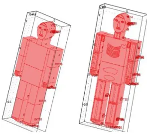
We adopted a 40-cylinder-segment model in 16 main segments as the geometric model of the human body.

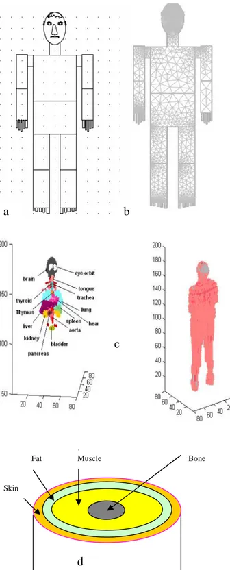
Fig. 1 (a) Body segment model (b) Meshed geometry

c) Concentric multilayered model for the hands, foots and all of end part of body. The head, neck, thorax, and abdomen segments have internal organ layers d) Schematic of the blood circulatory system model. In each layer, there is a pair of arterial and venous blood

pools corresponding to the arteriole, venules, and capillaries.

Each extremity segment (upper arm, forearm, hand, thigh, calf, and foot) is divided into four concentric layers: bone, muscle, fat, and skin [Fig. 1]. Each of the other segments (head, neck, thorax, and abdomen) has another layer on the inside of the bone corresponding to an internal organ. It is assumed that the properties of each layer are homogeneous and the longitudinal and angular coordinates are not taken into account. In each segment and layer, there are a large arterial blood pool and a venous blood pool corresponding to the main artery and the main vein, respectively. Heat transfer between two segments occurs through the large blood pools.

Mesh statistics:

Mesh statistics are: Number of freedom: 27062; Number of triangle: 13176; Number of boundary element: 1503; Number of vertex element: 183; Minimum element quality: 0.0894; Element area ratio: 8.13e-7

3 Human formulation

3.1. Thermal formulations

The bioheat equation is similar to the heat equation for heat conduction except that it splits the heat-source term on the right-hand side into three terms that are of interest in bioheat transfer problems. Further, the material properties in this equation are better suited to the study of heat transfer in tissue. The equation thus takes this form:

ext met b b b b t T ts..C._ .(kT) .C . (T T)Q Q  (1) Qext=Hab(r,t)[Tab(r,t)- T(r,t)] + Hvb(r,t)[Tvb(r,t)- T(r,t)]

Also, Hab: coefficient for heat transfer between tissue

and arterial blood per unit volume of tissue [W/(m3·K)], Hvb: coefficient for heat transfer between

tissue and venous blood per unit volume of tissue [W/(m3·K)], subscript b: blood, ab: arterial blood, and vb: venous blood.

We set Hab, Hvb, and Hav to be zero [30].

Where on the left-hand side:

• δts is a time-scaling coefficient (dimensionless).

• ρ is the tissue density (kg/m3).

• C is the specific heat of tissue (J/(kg·K)).

• k is the tissue’s thermal conductivity tensor (W/(m·K)).

On the right side of the equation, ρb Cb ωb (Tb − T) is

a source term for the blood perfusion where: • ρb is the density of blood (kg/m3).

• Cb is the specific heat of blood (J/(kg·K)).

• ωb is the blood perfusion rate (m3/(m3·s)).

Bone Muscle Fat Skin

d

a

b

c

• Tb is the arterial blood temperature (K).

Tab. 1 input data used in simulation and calculations

Finally, the second and third terms on the right side: • Qmet is the heat source from metabolism (W/m3).

• Qext is the spatial heat source (W/m3).

For a steady-state problem, the temperature does not change over time, and the first term in the bio-heat equation disappears.

3.1.1. Sub domain Settings

Table 1 shows the Sub domain Settings of the bio-heat equation application mode. The sub domain quantities are [2]:

Time-scaling coefficient: δts is normally 1, but we

change it to the time scale, from seconds to minutes by setting it to 1/60.

Density of tissue: The effective density of the tissue is for all practical purposes equal to the density of the tissue-blood continuum, since the vascular volume is much smaller than that of the solid tissue.

Specific heat of tissue: C describes the amount of heat energy required to produce a unit temperature change in a unit mass of tissue.

Thermal conductivity of tissue: k describes the relationship between the heat flux vector q and the temperature gradient Tas in:

q





k

.



T

Specific heat of blood: Cb describes the amount of eat

energy required to produce a unit temperature change in a unit mass of blood.

Blood perfusion rate: ωb describes the volume of

blood per second that flows through a unit volume of tissue.

Arterial blood temperature: Tb is the temperature at

which blood leaves the arterial blood veins and enters the capillaries.

Metabolic heat source: Qmet describes heat generation

from metabolism.

Spatial heat source: Qext describes heat generation

from an external source.

These quantities are the unit power per unit volume. The first term on the right side in (1) is the thermal conduction term. The second term shows the heat exchange between the entering arterial blood and the tissue through the capillary wall. Here it is assumed that perfect heat transfer between the blood in the capillary bed and the tissue occurs due to the extremely large surface area of the capillaries. In consequence, the temperature of the blood leaving the capillary bed is equal to the temperature of the tissue. However, this assumption does not hold for larger vessels.

Name EXPRESSION Description

rho_bone 6450[kg/m^3] Density of bone

rho_fat 810[kg/m^3] c_bone 840[J/(kg*K)] c_fat 3600[J/(kg*K)] k_bone 18[W/(m*K)] k_fat 0.512[W/(m*K)] k_b 0.543[W/(m*K)] T.C. blood sigma_bone 1e8[S/m] sigma_fat 0.333[S/m]

sigma_b 0.667[S/m] E.C., blood

omega_b 6.4e-3[1/s] B.p. rate

V0 1[V]

eps_diel 2.03 Relative permittivity,

dielectric (blood) rho_blood 1000[kg/m^3] C_blood 4200[J/(kg*K)] T_blood 37[°C ] k_skin 0.2[W/(m*K)] rho_skin 1200[kg/m^3] C_skin 3600[J/(kg*K)] wb_skin 3e-3[1/s] k_tissue 0.5[W/(m*K)] rho_tissue 1050[kg/m^3] C_tissue 3600[J/(kg*K)] wb_tissue 6e-3[1/s] Q_met 400[W/m^3] h_conv 10[W/(m^2*K)]

T_inf 10, 26 and 30 °C Ambient temperature

I0 1.4[W/mm^2]

Air velocity 0.1 m/s

Therefore, Qext, show the heat transfer through the

large vessels between the tissue and the arterial blood, and between the tissue and the venous blood. Over the entire body, however, the heat exchange efficiency through arteries or veins is apparently lower than that through capillaries.

Equations (2) and (3) are heat transfer equations for the arterial and venous circulatory system, respectively:

Arterial blood pool equation is:

)) , ( ) , ( ( )) , ( ) , ( ( ) , ( )) , ( ) , ( ( . ) , ( ) , ( . . ' ' t r T t r T H dV t r T t r T t r H t r T t r T C t r f t r V C ab vb av ab ab V ab ab am b b ab t T ab b b ab      



In addition, for venous blood pool:











Where V: blood pool volume [m3], V′: volume of tissue which the blood pool governs [m3], f: blood flow rate of blood pool [m3/s], and Hav: coefficient of

heat transfer between arteries and veins for counter current flow [W/K]. Subscript am: adjacent arterial blood pool, vn: adjacent venous blood pool.

The first term on the right side in (2) shows the transport of heat to the blood pool in question from the adjacent blood pool. The second term shows the heat exchange between the blood pool and the neighboring tissue. The third term expresses the countercurrent heat exchange between the artery and the vein. Equation (3) consists of the same terms, but the second term takes perfusion blood in tissue (wρbcb)

flowing into the venous blood pool into consideration. Skin surface heat is transferred by thermal radiation, conduction, and convection to the environment, and body heat loss is with sweat evaporation:

qs=qc+qr+qeva+qd (4)

Where qs: heat transfer rate at skin surface [W/m2], qc

: convective heat transfer rate [W/m2], qr : radiant heat

transfer rate [W/m2], qeva : evaporative heat transfer

rate [W/m2], qd : conductive heat transfer rate [W/m2].

The convective heat transfer rate is generally defined by using a convective heat transfer coefficient. In this study, the convective heat transfer coefficient for a cylinder was used [18], [19].

The radiant heat transfer rate follows Stefan-Boltzmann’s law [20], [21]. It is assumed here that evaporative heat loss is equal to insensible perspiration rate [22], [23] under conditions that induce little perspiration, such as room temperature.

Conductive heat transfer at the skin surface with a solid is not considered in this study. To simulate body temperature, it is necessary to solve the above equations simultaneously with an efficient algorithm and adequate property values.

3.1.2. Boundary Conditions

The boundary conditions for the Bioheat Equation are:

Boundary Condition Description

) ( ) .( k T q₀ hT_inf T n       _{Heat flux} 0 ) .(   n k T Insulation or symmetry T = T0 Prescribed temperature r = 0 Axial symmetry ) ( ) .(k1 T1 k2 T2 q0 hTinf T n       Heat flux discontinuity 0 ) .(k1T1k2T2  n Continuity

The boundary conditions on interior boundaries are: Heat Flux: heat flux condition accounts for a general heat flux, as well as that from convection as defined by a convective heat transfer coefficient. It interprets the heat flux in the direction of the inward normal. Therefore, a positive value of q0 corresponds to a heat

source.

• A positive value of q0 represents a heat source on the

boundary, for example a metabolism inflow of energy, such as radiation with specified intensity. Conversely, a negative value will represent a heat sink.

• The term h (Tinf – T) models convective heat transfer

with the surrounding environment, where h is the heat transfer coefficient and Tinf is the external bulk

temperature. The value of h depends on the geometry and the ambient flow conditions.

Insulation or symmetry: this condition applies to boundaries where the domain is well insulated. It can also be used to reduce model size by taking advantage of symmetry.

Prescribed temperature: T=T0, This boundary

condition prescribes the temperature T0.

Heat flux discontinuity: on interior boundaries an assembly pairs can specify a heat flux discontinuity, which is the same thing as a heat source or heat sink. The equation states that the difference between the heat flux on the left and the right is equal to the heat source on the boundary.

Continuity: in the absence of sources or sinks, that condition specifies that the heat flux in the normal direction is continuous across the boundary. This

boundary condition is only for interior boundaries and for assembly pairs at boundaries between parts of an assembly.

3.2. Human Magnetic Formulation

The governing equation for the nerves in the tissue and blood vessels is:

j e _Q J V     .( ) (4) Where V is the potential (V), σ the electric conductivity (S/m), Je an externally generated current density (A/m2), Qj the current source (A/m3).

The boundary conditions at the cylinder’s outer boundaries is ground (0 V potential). Assume continuity for all other boundaries.

V=0 on the wall and V=V0 on the related tissues.

n.(J1-J2)=0 on all other boundaries.

) ( ) ( _, j t kz rZ C kz t j r C r e H e e e E   _  (5)



Where z is the direction of propagation, and r, φ, and z are cylindrical coordinates centered on the axis of the tissues. Pav is the time-averaged power flow in the

tissue; Z is the wave impedance in the dielectric of the blood and tissue, while rinner and router are the bone and

tissue radius, respectively. Further, ω denotes the angular frequency. The propagation constant, k, relates to the wavelength of axon in the medium, λ, as: k=2π/ λ.

In the tissue actually in nerves, the electric field also has a finite axial component whereas the magnetic field is purely in the bone direction. Thus, it can model the tissue using an axisymmetric transverse magnetic (TM) formulation. The wave equation then becomes scalar in Hφ: 0 ) ) (( 1 ₀ 0         _{ }    _r j H _rk H ₍₇₎

The boundary conditions for the bone surfaces are: nH=0

The feed point is modeled using a port boundary condition with a power level set to 10 W/m3. This is essentially a first-order low-reflecting boundary condition with an input field Hφ0:

0 2 _ 







H





For an input power of Pav deduced from the

time-average power flow.

The nerves and blood dipoles flux radiates into the tissue where a damped wave propagates. Because it can discretize only a finite region, it must truncate the geometry some distance from the tissue for nerves carrier using a similar absorbing boundary condition without excitation. Apply this boundary condition to all exterior boundaries. Finally, apply a symmetry boundary condition for boundaries at r = 0: E_r0,

0    r Ez .

In other hand, the external heat source can be equaled to the resistive heat generated by the electromagnetic field: Qext=0.5*Re[(σ-jω)E*ET]. Results are shown in

Fig.s 3 and 6.

The model assumes that the blood perfusion rate is ωb

= 0.0036 s-1, and that the blood enters the liver at the body temperature Tb = 37 °C and is heated to a

temperature, T. The blood’s specific heat capacity is Cb = 4200-3639 J/(kg·K), it is the best to take account

of 4200.

4 Numerical Calculation

The numerical calculation outline of the bio-heat transfer equations is as follows:

1)Using of cylindrical and Cartesian coordinates; 2) using finite difference method to discritizations 3) using of time dependent solver with to different time solving, 60 and 88 minutes in transient and stationary mode; 4) rung-kutha method is used to iterations. The detailed method is presented in [10], [11]. As a

result, the developed computer program

simultaneously calculates the distributions of magnetic fields, current density, internal temperature, heat flux, and blood temperature of all segments with time by inputting thermal environmental factors such as air temperature, mean radiant temperature, air velocity, and relative humidity of each segment. Voltage produced due to chemical interactions in blood, tissues and electric and magnetic signals in axons, dendrites and nerves& neurons are considered.

4.1. Blood flow rate

A human thermal model needs to include a program for thermoregulation that mainly consists of three regulation systems: Skin blood flow (SBF) regulation, perspiration and thermo genesis.

Actually, SBF regulation plays a significant role along with the thermal neutral zone of the human body [24]. Since there is no trial data about SBF regulation over the whole body, we used (9) for all segments of the human body according to the empirical equations for SBF of the forearm [25]-[28]:





i T T T T SBF

Where (SBF)i: skin blood flow rate of the ith segment

of the human body [ml/(100ml·min)], Thy:

hypothalamic, temperature [K], Tsm: mean skin

temperature [K], Thy0: set point of Thy [K], Tsm0: set

point of Tsm [K], (SBF0)i: skin blood flow rate in

comfort of the ith segment [ml/(100ml·min)], ζi: coefficient for skin blood flow regulation of the ith segment [−]. Values of ζi are; head: 1.6, neck: 1,

thorax: 1.4, abdomen: 1, upper arm: 1.4, forearm: 1, hand: 2.4, thigh: 0.8, calf: 1.2, foot: 2 [29].

In the coding of computer, the numerical calculation of the bio-heat transfer equation is performed for each time, SBF is renewed by input of up-to-date Thy and

Tsm. However, there are some problems with (9), a

simple linear equation, that need to be discussed. The SBF model must be improved to incorporate the results obtained in the latest physiological research.

5 Simulation and Calculation Results

and Discussions

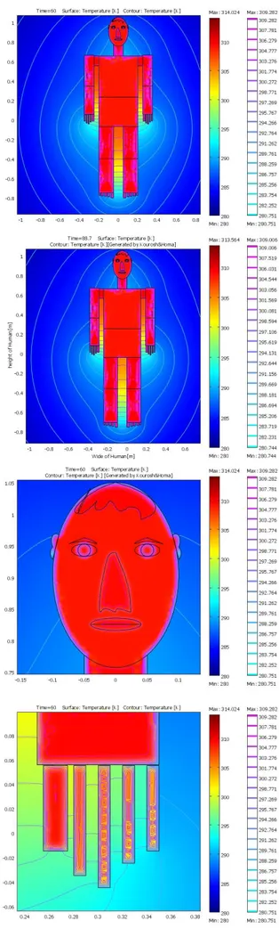
Fig. 2 and 7 shows the results of body temperature simulated under the condition that both the air temperature and the mean radiant temperature were maintained at 30 °C for a 60-min period, then changed to 26°C and maintained at that temperature for a subsequent 28-min period. The skin surface temperatures of body segments at 60 min and at 88 min are shown in Fig. 2, respectively. The geometry for temperature simulation is a profile and section, just to show of skin, fat and tissues temperatures.

As can be seen, the skin surface temperatures of the peripheral segments were lower than the trunk. The mean skin temperatures at 60 min and at 88 min are 35.1 °C and 33.3 °C, respectively.

Fig. 6 shows that the decreasing rates of the skin surface temperature vary among the segments chiefly because their thermal capacities and metabolic heat production rates are different. The diminution from 60 min to 88 min of the core temperature (hypothalamic temperature) is 0.8 °C, which is much smaller than that of the skin surface temperatures. For this reason, face has a homogonous temperature profile, in Fig. 2. Here, we present a few comments on how SBF regulation affects the temperature of each region. The SBF-regulated hypothalamic temperature (Fig. 2) was 1.35 °C higher than the non-regulated temperature [(9) was not used] at 88 min.

Fig.2. Simulated body temperature profile with

detailed segments, from top to bottom Fig.s are: temperature profile in 60 min, temperature profile in 88 min, head and face temperature distribution, hand fingers and finally foot temperature distributions.

The SBF- regulated skin surface temperature of the thigh was 2.36 °C lower than the nonregulated temperature at 88 min. That is to say, when SBF decreased, the skin surface temperature was lowered and the heat loss from the body surface was inhibited.

Fig. 3 Simulated body magnetic fields profile with

detailed segments, from top to bottom Fig.s are: magnetic energy density, magnetic field for 1 min and

2 v, magnetic field for 88.7 min, foot fingers, head, abdomen and chest, magnetic field for 1 min and 1 v.

Fig. 4 shows the simulated internal temperature profiles of the head, forearm, thigh, and foot. It is obvious that the form of the temperature profile varies among the segments. Especially in the head, since the brain has relatively large blood flow and metabolic rates, it can be seen that the internal temperature is constant (309.28 K at 60 min). It is difficult to verify the simulated internal temperature profiles because there is far less measurement data on internal temperature than on skin surface temperature. We therefore have to discuss the data validity based on fragmentary data.

Using traced Fig. 4 by governing equations, mathematically formulae has been generated for scrotum to top of head, magnetic field in norm and temperature are:

Mag.(x) = 1.0566e-020*x^10- 1.0373e-017*x^9 +4.3143e-015*x^8 -9.9045e-013*x^7 +1.3708e010*x^6 1.1727e008*x^5 +6.1106e007*x^4 -1.8408e-005*x^3 +0.00029387*x^2 -0.0023614*x + 0.014194

Norm of residuals =0.021528

Temp.(x)= 8.9742e-020*x^10 -1.1063e-016*x^9 +

5.684e-014*x^8 -1.5962e-011*x^7

+2.6916e009*x^6 2.8132e007*x^5+ 1.8141e005*x^4 -0.00069569*x^3+ 0.014674*x^2- 0.14646*x + 309.25 Norm of residuals = 6.7695

Authors to sake of paper pages limitations forbear of other equations to write here.

0 20 40 60 80 100 120 140 160 180 200 300 301 302 303 304 305 306 307 308 309 310

Generated by Kourosh & Homa

Per unit of body members

T e m p e ra tu re [ K ]

Scrotum to top of head Acros of two thghs (foot) Forearm 0 20 40 60 80 100 120 140 160 180 200 10-4 10-3 10-2 10-1

Per unit of body members

M a g n e ti c f ie ld s , n o rm Generated by Kourosh&Homa

Scrotum to top of head Across of foot fingers Top side of food

Hand fingers from small finger to thumb

Fig. 4 Magnetic fields in norm (a) and temperature

distribution in across of body members (b)

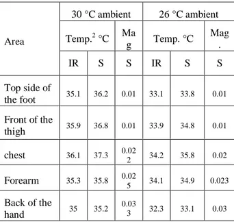
Fig. 5. IR images1 of 1) the top side of the foot, 2) the front of the thigh, 3) the chest, 4) the forearm, and 5)

the back of the hand remaining in a 30 °C ambient temperature environment for 60 min (a) and

IR image: courtesy Dr. John Keyserlingk

1 2 3 4 5

subsequently remaining in a 26°C environment for 60 min (b). A temperature colour legend of the same scale is used in (a), (b) (1: 31.0-36.0 °C; 2-5: 32.0-37.0 °C). C) Simulated temperature for 60 min and 30

°C ambient temperature. The number in the table 2 represents the temperature at the symbol “-” Fig.s 4 was a healthy male (age = 36 years; height = 172 cm; weight = 73 kg). Fig.s 5(a) and (b) displays the IR images at 60 min for 26 and 30 °C and (c) shown the simulation results.

Fig. 6 Slice of the head, magnetic resonance field

projection distributions

Generated by Kourosh & Homa

20 25 30 35 40 0 20 40 60 80 100 Time [min] T e m p e ra tu re [ o C ] Hypothalamous thorax thigh forearm foot

Fig. 7: Hypothalamus temperature (temperature at the

centre of the head) and skin surface temperatures of four segments with time.

Tab. 2 Comparisons of temperature and magnetic

fields in norm. At the symbol “-” on Fig. 4.

6 Conclusions

To evaluate magnetic and thermal behavior of human obtained under various environmental conditions, authors proposed a human thermal and magnetic simulation and calculation with verification of IR images. The model was based on a numerical calculation of the bio-heat transfer and electric- magnetic equations that express heat transfer and electromagnetic phenomena within the human body. A 16-cylinder&cartesian-segment upgraded to 40 segments model was used as the geometry of the human body. Skin, tissue, fat and bone are considered to more part of body. Comparisons of simulation and calculation results with their IR images, Fig. 5, in thermal mode indicate that this method is effective in eliminating the influence of the thermal environmental conditions. However, the difference between the simulated model and images is related to boundary data and formulation of soft wares. In future work, we will use this method to investigate of several subjects under various thermal and magnetic environments with respect to multilayer segments, electrolysis in blood and to find the accurate formulation for neurons.

5. References

[1] Kourosh mousavi Takami, Effects of

electromagnetic and electric fields on human health, Kahroba journal (specialized in power electric engineering), April 1998.

[2] Comsol version 3.4 a, Stockholm, Sweden. [3] R.B. Roemer and T.C. Cetas, Applications of bioheat transfer simulations in hyperthermia, Cancer Res., vol. 44, pp. 4788-4798, 1984.

[4] A. Shitzaer and R.C. Eberhart, Eds., Heat Transfer in Medicine and Biology. New York: Plenum, 1985. [5] G.M.J. Van Leeuwen, A.N.T.J. Kotte, and J.J.W. Lagendijk, A flexible algorithm for construction of 3-D vessel networks for use in thermal modeling, IEEE Trans. Biomed. Eng., vol. 45, pp. 596-604, 1998. [6] R.G. Gordon, R.B. Rober, and S.M. Horvath, Mathematical model of human temperature regulatory system-transient cold exposure response, IEEE Trans. Biomed. Eng., vol. 23, pp. 434-444, 1976.

[7] S. Yokoyama and H. Ogino, Developing computer model for analysis of human cold tolerance, Ann. Physiol. Anthropol., vol. 4, pp. 183-187, 1985. [8] A.P. Gagge, J.A.J. Stolwijk, and Y. Nishi, An effective temperature scale based on a simple model of human physiological regulatory response, ASHRAETrans.,vol.77,pp.247-262,1971.

[9] P.O. Fanger, Thermal Comfort. Copenhagen, Denmark: Danish Technical Press, 1970.

[10] S. Yokoyama, N. Kakuta, and K. Ochifuji, Development of a new algorithm for heat transfer

30 °C ambient 26 °C ambient Temp.2 °C Ma g Temp. °C Mag . Area IR S S IR S S Top side of the foot 35.1 36.2 0.01 33.1 33.8 0.01 Front of the thigh 35.9 36.8 0.01 33.9 34.8 0.01 chest 36.1 37.3 0.02 2 34.2 35.8 0.02 Forearm 35.3 35.8 0.02 5 34.1 34.9 0.023 Back of the hand 35 35.2 0.03 3 32.3 33.1 0.03 30e-3 20e-3 15e-3 10e-3 5e-3 1e-4 G en er at ed b y K o u ro sh & H o m a

equation in the human body and its applications, Appl. Human Sci., vol. 16, no. 4, pp. 153-159, 1997. [11] S. Yokoyama, N. Kakuta, T. Togashi, Y. Hamada, M. Nakamura, and K. Ochifuji, Development of prediction computer program of whole body temperatures expressing local characteristic of each segment, Part 1—Bio-heat equations and solving method, (in Japanese), Trans. SHASEJapan, vol. 77, pp. 1-12, 2000.

[13] H.H. Pennes, Analysis of tissue and arterial blood temperatures in the resting human forearm, J. Appl. Physiol., vol. 1, pp. 93-123, 1948.

[14] H. Arkin and A. Shitzer, A model of thermoregulation in the human body, presented at ASME Winter Annual Meeting, New Orleans, LA, paper no. 84-WA/HT-66, 1984.

[15] J.W. Baish, P.S. Ayyaswamy, and K.R. Foster, Heat transport mechanisms in vascular tissues, ASME J Biomech. Eng., vol. 108, pp. 324-331, 1986. [16] H. Arkin, L.X. Xu, and K.R. Holmes, Recent developments in modeling heat transfer in blood perfused tissues, IEEE Trans. Biomed. Eng., vol. 41, pp. 97-107, 1994.

[17] E.H. Wissler, A mathematical model of the human thermal system, Bull. Math. Biophysics, vol. 26, pp. 147-166, 1964.

[18] P.H. Oosthuizen and S. Madan, Combined convective heat transfer from horizontal cylinders in air, ASME J Heat Transfer, vol. C-91, pp. 194-196, 1970.

[19] A. Bejan, Heat Transfer, Wiley, 1993

[20] M.L. Toison, Infrared and Its Thermal Applications. The Netherlands: Philips Tech. Lib., 1964.

[21] N. Kakuta, S. Yokoyama, M. Nakamura, and K. Mabuchi, Estimation of radiative heat transfer using a geometric human model, IEEE Trans. Biomed. Eng., vol. 48, pp. 324-331, 2001.

[22] Y. Kuno, Human Perspiration. Springfield, IL: Charles C. Thomas, 1956.

[23] K. Ohara and T. Ono, Regional relationship of water vapor pressure of human body surface, J. Appl. Physiol., vol. 18, pp. 1019-1022, 1963.

[24] H. Hensel, Thermo reception and Temperature Regulation. London and New York: Academic, 1981. [25] C.R. Wyss, G.L. Brengelmann, J.M. Johnson, L.B. Rowell, and M. Niederberger, Control of skin

blood flow, sweating, and heart rate: Role of skin vs. core temperature, J. Appl. Physiol., vol. 36, no. 6, pp. 726-733, 1974.

[26] C.R. Wyss, G.L. Brengelmann, J.M. Johnson, L.B. Rowell, and M. Niederberger, Altered control of skin blood flow at high skin and core temperature, J. Appl. Physiol., vol. 38, no. 5, pp. 839-845, 1975. [27] C.B. Wenger, M.F. Roberts, J.A.J. Stolwijk, and E.R. Nadel, Forearm blood flow during body temperature transients produced by leg exercise, J. Appl. Physiol., vol. 38, no. 1, pp. 58-63, 1975. [28] M.V. Savage and G.L. Brengelmann, Control of skin blood flow in the neutral zone of human body, J. Appl. Phys., vol. 80, no. 4, pp. 1249-1257, 1996. [29] S. Yokoyama, N. Kakuta, T. Togashi, Y. Hamada, M. Nakamura, and K. Ochifuji, Development of prediction computer program of whole body temperatures expressing local characteristic of each segment, Part 2—Analysis of the mathematical model for the control of skin blood flow, (in Japanese), Trans. SHASE Japan, vol. 78, no. 1-8, 2000.

[30] Naoto Kakuta, Shintaro Yokoyama, and Kunihiko Mabuchi, Human Thermal Models for Evaluating Infrared Images, IEEE engineering in medicine and biology, November 2002.

Appendix:

Fig. 8 3D body model of Fig. 1a