L
INAA
NDERSSON,
M
ATSH
AMMARSTEDT&
E
MMAN
EUMAN2012-8
Residential mobility, tipping
behaviour, and ethnic
segregation: Evidence from
Sweden
Abstract
This paper studies tipping behaviour in residential mobility of the native population in Sweden between 1990 and 2007. Using regression discontinuity methods, we find that the growth in native population in a neighbourhood discontinuously drops once a neighbourhood’s immigrant share exceeds the identified tipping point. In the 1990s the drop can be attributed both to increased out-migration of natives (native flight) and decreased in-migration of natives (native avoidance). In 2000-2007, native flight appears to be driving the segregation pattern. Thus, the native residential mobility has contributed to increased ethnic segregation in Sweden between 1990 and 2007.
Contact information
Lina Andersson
Centre for Labour Market and Discrimination Studies Linnaeus University
SE-351 95 Växjö lina.andersson@lnu.se Mats Hammarstedt
Centre for Labour Market and Discrimination Studies Linnaeus University
SE-351 95 Växjö
mats.hammarstedt@lnu.se Emma Neuman
Centre for Labour Market and Discrimination Studies Linnaeus University
SE-351 95 Växjö emma.neuman@lnu.se
1. Introduction
The question of immigrants’ location choices in the host country has received the attention of researchers in the past few decades.1 The United States and several countries in Europe, have experienced a large inflow of immigrants into certain geographical areas and cities leading to ethnic segregation. The driving forces behind this ethnic segregation, the presence of ethnic enclaves and their importance for the economic success among the foreign born has been widely studied.2 Researchers have long been interested in the dynamics of segregation. Shelling (1971) used social interaction models to explain segregation and argued that the ethnic mix in a certain neighbourhood might change when natives’ willingness to pay for housing decreases as the number of members of ethnic minorities residing in that neighbourhood increases. Card, Mas and Rothstein (2008) introduce a model in which an ethnically mixed neighbourhood remains stable until the ethnic minority reaches a certain tipping point. When the share of the ethnic minority in the neighbourhood exceeds this tipping point, the natives will begin to leave the neighbourhood. When applying their model to US data, Card, Mas and Rothstein documented tipping-like behaviour among natives in several US cities. Further, they found that native tipping behaviour varied among cities with different attitudes towards ethnic minorities.
This paper examines the driving forces behind ethnic geographical segregation in Sweden.3 What role has native residential mobility played in the process of ethnic segregation during the 1990s and 2000s? We use register data from 1990, 2000, and 2007 to identify municipality-specific tipping points and to study tipping behaviour in Sweden's 12 largest municipalities. Sweden is a suitable testing ground for analysing tipping behaviour for several reasons. Firstly, Sweden has a long history of immigration. In 2012 about 14 per cent of Sweden’s total population was foreign born. Secondly, the character of immigration to Sweden has changed. The great majority of immigrants coming to Sweden today are refugees and ‘tied movers’ from Asia, Africa and the Middle East. Apprehensions about the fact that these immigrants should prefer to settle in neighbourhoods with a large share of immigrants from their own group have often been expressed. Thirdly, discrimination against ethnic discrimination in the Swedish housing market is well documented.4 Thus, we have good reasons to believe that natives tend to avoid or move out of areas with a large share of inhabitants from certain ethnic groups.
Our empirical analyses proceed as follows: We apply the method introduced by Card, Mas and Rothstein (2008) in order to identify municipality-specific tipping points. We then use regression discontinuity methods to quantify the effect of the tipping points on growth in the native population. In addition, we explore the extent to which the (possible) decrease in native population growth is driven by native flight (i.e. increased out-migration), and/or native avoidance (i.e. reduced in-migration of natives).5
1 See Bartel (1994), Borjas (1999), Åslund (2006).
2 See Cutler, Glaeser and Vigdor (1999), Bayer, McMillan and Reuben (2004) and Edin, Fredriksson and
Åslund (2003).
3 For Swedish research on ethnic segregation and its implications on labour market outcomes and school
achievement, see e.g. Nordström Skans and Åslund (2010) and Edin, Fredriksson, Grönkvist and Åslund (2011).
4 See Ahmed and Hammarstedt (2008), Ahmed, Andersson and Hammarstedt (2010).
5 The relative importance of native flight and native avoidance to the increased immigrant concentration
We find support for tipping behaviour in a majority of the 12 largest municipalities in Sweden. Furthermore, we see a large heterogeneity in the identified value of the immigrant shares at which the society tips. The results give clear evidence that the native population growth responds discontinuously to the initial immigrant share around the tipping point. The drop in the growth rate of the native population around the tipping point was 7.7 per cent in the 1990s and 3.1 per cent in the 2000s. We find that this drop in the native population growth rate around the tipping point during the 1990s is related to a native flight from areas with a large proportion of immigrants. The results also indicate that natives avoided moving in to neighbourhoods with high immigrant populations during the 1990s. This explanation for the increased segregation during the 1990s is about equally important as the flight story. In the 2000s, an increased out-migration rate of natives from neighbourhoods with a high immigrant concentration seems to be driving the segregation pattern.
The paper is organised as follows. Section II offers an overview of immigration to Sweden and the changes in the composition of the immigrant population since the Second World War. Section III provides the theoretical framework and Section IV presents the data. Section V presents the empirical models and Section VI explains the results. Section VII summarises and concludes.
2. Immigration and the immigrant population in Sweden
Both the size and composition of Sweden's immigrant population has changed during the last decades. In 1940 only about 1 per cent of the country's total population had been born abroad. In 1970, this share had risen to 7 per cent. In 2012 about 14 per cent of Sweden's population is foreign born. After 1945, and at some times during the 1950s and 1960s, refugees from Eastern Europe moved into Sweden. But most of the immigration to Sweden from the 1950s until the mid-1970s was labour-force migration as a result of the country’s industrial and economic expansion. The labour-force migration consisted primarily of poorly educated immigrants from Finland, former Yugoslavia, Italy and Greece. During the 1950s and 1960s labour-force migrants also came from other Nordic countries and from countries in Western Europe such as West Germany.
In the mid-1960s, Swedish trade unions accused immigrants of depressing wages for low paid workers. A more restrictive immigration policy and the deterioration of the labour market situation changed the character of immigration during the 1970s. As the labour-force migration of European immigrants tapered off, the number of refugees from non-European countries started to increase. In the mid-1970s, refugee migration from Latin America started to reach significant proportions, and during the 1980s a much larger number of refugees came from Asia and Africa. During the 1990s, refugee migration continued, but now dominated by refugees from former Yugoslavia and the Middle East. Refugee migration from countries in the Middle East has continued into the 21st century.
native avoidance can be attributed to the increased immigrant concentration, native avoidance appears to be the main driving force.
The composition of the immigrant population has likewise changed. In 1970 about 60 per cent of Sweden's foreign-born population had been born in other Nordic countries and about 30 per cent in other European countries. Only about 5 per cent were born outside Europe. In 2008 only about 20 per cent were born in other Nordic countries, about 36 per cent were born in other European countries, and almost 43 per cent of the immigrant population were born in non-European countries.
Table 1: The composition of the foreign-born population living in Sweden 1960-2008
Region of birth 1960 1970 1980 1990 2000 2008 Nordic countries 58.1 59.7 54.4 40.3 27.9 21.0 Other European countries 37.0 34.9 33.8 32.1 32.9 35.8 Non-European countries 4.9 5.4 11.8 27.6 39.2 43.2 Total 100.0 100.0 100.0 100.0 100.0 100.0
Source: Statistics Sweden, Statistical Yearbook and Population Statistics, different volumes.
Thus, the share of foreign-born individuals with a non-European background greatly increased. Further, recently arrived immigrants tend to settle in metropolitan areas such as Stockholm, Gothenburg and Malmo or in other large municipalities. According to Statistics Sweden (2008) more than 90 per cent of the immigrants in the 1997–2002 cohort resided in cities or metropolitan areas five years after their immigration.
The increased share of visible minorities originating from non-European countries combined with the concentration of such immigrants in metropolitan areas or in large municipalities give us reason to believe that this may have affected residential mobility among natives in such municipalities.
3. Theoretical framework
Why should we expect tipping behaviour among the native population in Sweden? As a starting point for our analysis we use the theoretical model developed by Card et al (2008) to explain tipping behaviour in a neighbourhood. The model is depicted in Figure 1.
Assume a neighbourhood with a homogenous stock of housing to which there are two potential buyers: a native and an immigrant. Suppose further that the demand for housing or the willingness to pay of natives and immigrants, bnatives and bimmigrants, respectively, depend on the share of immigrants, m, residing in the neighbourhood. The share of natives already residing in the neighbourhood is (1-m).
At relatively low immigrant shares, it is assumed that natives’ willingness to pay for housing increases as m rises and that it decreases when the immigrant share reaches some critical level as shown in Figure 1. Thus, as long as the share of immigrants is low, natives do not mind having immigrant neighbours but as the share becomes sufficiently high natives come to resent having immigrant neighbours. For the sake of
simplicity, the immigrants’ willingness to pay for housing is assumed to be negatively related to the share of immigrants.
There are three possible equilibria of the native-immigrant composition in a neighbourhood: one all-immigrant and two mixed. As long as natives’ willingness to pay increases with the immigrant share, (i.e. as long as the immigrant share is sufficiently low), the neighbourhood will be mixed for any given level of immigrants’ demand for housing, as in point (i) in Figure 1. This is a stable equilibrium, since if the immigrant share were to increase due to some demand shock, it would eventually return to point (i) as natives would outbid immigrants due to their higher willingness to pay. The same reasoning holds to the left of point (i), where immigrants would outbid natives.
If, however, the immigrant share in the neighbourhood is such that natives’ willingness to pay is decreasing, as in point (ii), the neighbourhood will be mixed but it will not be at a stable equilibrium. If a demand shock pushes the neighbourhood out of the equilibrium, it will not return to point (ii), but will instead move towards one of the other two equilibria (i) and (iii). For example, if the immigrant share rises above that given by point (ii), immigrants will outbid natives, since the willingness to pay is higher among immigrants than among natives, and the neighbourhood will move towards a stable all-immigrant equilibrium, point (iii).
What then happens if there is an exogenous inflow of immigrants? Assume for simplicity an all-native neighbourhood as illustrated in Figure 2. Suppose further that inflow of immigrants is such that it continuously increases immigrants’ demand for housing in the neighbourhood. As a result, the immigrant demand curve will shift
(ii) (i) (iii) 0,5 1 0 Immigrant Housing Price bnatives bimmigrants Figure 1
upwards. As long as natives’ willingness to pay for housing increases, there will be a mixed neighbourhood; the more immigrants’ demand for housing increases, the higher the minority share in the neighbourhood. The highest immigrant share at which the neighbourhood remains mixed is the share at which the demand curve of natives and of immigrants are tangential. If immigrants’ housing demand continues to increase, the immigrant share passes this critical value and the neighbourhood experiences tipping. In other words, the demand for housing of natives decreases and the only stable equilibrium is an all-immigrant neighbourhood.
The immigrant share at the tangency point is the tipping point, m*. The location of the tipping point depends on the native population's tolerance of immigrant neighbours; the stronger the preferences among natives against immigrant neighbours are, the lower the tipping point is expected to be.
This theoretical model gives us good reason to expect that the large inflow of non-Western immigrants to Sweden in the last 20 years may have generated a shock in immigrants’ demand for housing, resulting in tipping behaviour of the native population. Further, previous research has documented ethnic discrimination on the Swedish housing market, indicating that natives do have some prejudice against having immigrant neighbours.6
6
Ahmed and Hammarstedt, 2008; Ahmed, Andersson and Hammarstedt, 2010.
0,5 1 0 Immigrant share Housing Price (ii) (iii) bnatives bimmigrants bimmigrants’ Figure 2 m*
4. Data
We study tipping behaviour in the 12 largest Swedish municipalities in 2007: Stockholm, Göteborg, Malmö, Uppsala, Linköping, Västerås, Örebro, Norrköping, Helsingborg, Jönköping, Umeå, and Lund.7 The municipality of Stockholm is too small to be representative for the city of Stockholm and therefore we study Stockholm at the county level. We focus on changes in the native population growth between 1990 and 2000 and between 2000 and 2007.
In order to study tipping behaviour within these municipalities, we use individual data from the register-based longitudinal data base LISA (Longitudinal Integration Database for Health Insurance and Labour Market Studies) developed by Statistics Sweden. We have information on neighbourhood of residence of all individuals living in Sweden, 16 years and older, as well as on their demographic characteristics, labour market characteristics, and use of social benefits in the years 1990, 2000, and 2007.
Neighbourhoods are based on SAMS areas (Small Area Market Statistics). The SAMS areas were created by Statistics Sweden and are the finest geographical division that can be obtained for Sweden. These geographical areas were created to be homogenous in terms of type of housing, household income, and educational attainment. In total, there are 9,200 SAMS in Sweden and with an average of 1, 000 inhabitants. In the 12 municipalities included in this study, there are 3,135 SAMS areas in 1990, 3,203 in 2000, and 3,233 in 2007. In order to obtain neighbourhood units that are consistent over time, we only include SAMS areas that are present in the data set in 1990, 2000 and in 2007. We also exclude "redundant neighbourhoods" that were too heterogeneous to be classified as SAMS areas. After these selections, the total number of neighbourhoods is 3,053 in 1990, 2000, and in 2007.
In order to identify unique tipping points, the neighbourhoods must be homogenous. Therefore, we impose a number of restrictions in order to increase the homogeneity of the neighbourhoods over the two time periods under consideration. First, we exclude sparsely populated SAMS areas and focus on neighbourhoods with more than 200 inhabitants. Second, following Card et al (2008) we exclude outliers in terms of neighbourhood population growth by restricting the analysis to SAMS areas with 1) a native population growth in each period that is less than five times higher than the base-year total population and 2) a total population growth in each period that is less than five standard deviations higher than the average population growth in the municipality. After these restrictions, the sample used to study tipping behaviour comprises 2,277 neighbourhoods in 1990-2000 and 2,414 neighbourhoods in 2000-2007.
In the empirical analysis we explore how natives and Western immigrants respond to the share of non-Western immigrants in their neighbourhood. We choose this grouping because we want to study tipping behaviour in relation to an influx of visible ethnic minorities. Moreover, Western immigrants are doing relatively well on the Swedish labour market and are not subjected to the sort of discriminatory treatment which has been documented for non-European immigrants.8
7
See SCB, Befolkning. Folkmängden efter kommun, civilstånd och kön. År 1968-2010. http://www.ssd.scb.se/databaser/makro/Produkt.asp?produktid=BE0101. In 1990, the only difference in the order of the cities is that Borås and Sundsvall is marginally larger than Umeå and Lund.
8 See e.g. Bevelander and Skyt Nielsen , 2001; Hammarstedt and Shukur, 2007; Carlsson and Rooth,
Thus, we divide the sample into two groups: natives (comprising both natives and individual of a Western origin), and immigrants (comprising individuals of a non-Western origin). An individual is defined as native if he/she was born in Sweden and if his/her parents had also been born in Sweden. We define an individual as a Western immigrant if he/she is resident in Sweden and born in a Western country (including Western Europe, the US, Canada, and New Zealand). An individual is also defined as a Western immigrant if he/she was born in Sweden and if at least one of the parents was born in a Western country. An individual is considered to be a non-Western immigrant if he/she was born in a non-Western country (Southern Europe, Eastern Europe, Africa, Asia and Latin America).9 An individual is also defined as a non-Western immigrant if he/she is born in Sweden and if at least one of the parents is born in a non-Western country. Individuals born in Sweden with one parent born in a Western country and the other born in a non-Western country are also defined as non-Western immigrants. In the remainder of the analysis, natives and Western immigrants will be referred to as natives and non-Western immigrants will be referred to as immigrants.
Table 2 presents summary statistics of the sample at the neighbourhood level. It emerges that, on the one hand, between 1990 and 2000 the average share of immigrants in the neighbourhoods rose from 8 per cent to almost 13 per cent. The average growth in the native population has, on the other hand, slightly decreased from 3 per cent to about 2 per cent between the two time periods. There has also been a decrease in the average growth in the total population from 9 per cent to nearly 7 per cent.
Table 2 also shows the growth in the total and native population, in neighbourhoods with different shares of non-Western residents. It is interesting to note that between 1990 and 2000 neighbourhoods became more immigrant-dense. In 1990, nearly 43 per cent of the neighbourhoods had an immigrant share of less than 5 per cent and in 2000 this share had decreased to about 25 per cent. At the same time, the share of neighbourhoods with an immigrant share larger than 5 per cent increased. The largest increase is observed for neighbourhoods with an immigrant share larger than 20 per cent; in these neighbourhoods the share more than doubled.
9
Table 2: Descriptive statistics of the neighbourhoods included in the sample
1990 2000
Mean % immigrants, base year 8.0 12.8
Growth in total population, t-1* to t (%) 9.0 6.5
Growth in native population, t-1 to t as % of
t-1 population 3.0 1.6
0% -5% immigrants in base year
% of SAMS areas in sample (number) 42.3 (964) 24.6 (595)
Growth in total population 9.1 6.8
Growth in native population 6.6 6.7
5% -20% immigrants in base year
% of SAMS areas in sample (number) 50.8 (1157) 57.9 (1397)
Growth in total population 9.4 5.5
Growth in native population 2.2 1.2
20% -40% immigrants in base year
% of SAMS areas in sample (number) 6.0 (134) 12.6 (305)
Growth in total population 6.1 6.0
Growth in native population –11.4 –3.7
40% -100% immigrants in base year
% of SAMS areas in sample (number) 1.0 (22) 4.8 (117)
Growth in total population 3.6 8.0
Growth in native population –17.6 –5.0
Number of SAMS areas in sample 2,277 2,414
Note: *t-1 refers to the base year in each period, i.e. 1990 for the first and 2000 for the later, while t is the last year of the period, i.e. 2000 for the first and 2007 for the second period.
Table 2 shows that the growth rate of the native population differs among the four subgroups. In neighbourhoods with an immigrant share less than 20 per cent, the native population is growing in both time periods while it is decreasing in neighbourhoods with relatively larger immigrant shares. In neighbourhoods with the lowest immigrant share, the native population growth rate amounted to about 7 per cent during the two time periods and to about roughly 2 per cent in neighbourhoods with a somewhat larger immigrant share. In the two more immigrant-dense subgroups, the native population decreased by 8 per cent and 13 per cent, from between 1990 and 2000. Between 2000 2007, the negative growth rate of the native population in these neighbourhoods was lower and amounted to about 4 and 5 per cent.
5. Empirical specification
Identification of tipping points
We follow the method employed by Card et al (2008) to identify municipality-specific tipping points. The one-sided tipping model predicts that the share of natives should fall discontinuously once the minority share passes some critical value. Following Card et al (2008) we apply a method similar to those used for the identification structural breaks in time series analysis to identify this unknown critical value of the minority share of the 12 Swedish municipalities.
We estimate a model that relates the mean per centage change in native population of neighbourhood i in municipality c in 1990-2000 and in 2000-2007 to the share of immigrants in the base year of each time period. Let m*c,t1 denote the
municipality-specific tipping point where t–1 is the base year (= 1990, 2000). We allow the candidate tipping point to be located between minority shares of 1 to 60 per cent. For each candidate tipping point, we estimate the following regression model for each municipality, c, and for each time period:
ict ct
ict c c t c i d m m dn, , 1 ,,1 *,1 ,, (1).The dependent variable, dni,c,t, is the growth rate of the neighbourhoods’ native population in each municipality and in each time period. Specifically,
,, ,, 1
, , 1 ,,ct ict ict / ict
i N N P
dn where Ni,c,t is the number of native residents of
neighbourhood i in municipality c in the year t (= 2000, 2007), Ni,c,t1 is the number of native residents in the base year t–1 (=1990, 2000), and Pi,c,t1 is the neighbourhood’s
total population in the base year. mi,c,t1 is the base-year share of non-Western immigrants of neighbourhood i in municipality c. Specifically, mi,c,t1 Mi,c,t1/Pi,c,t1
whereMi,c,t1 is the number of non-Western immigrants of neighbourhood i in municipality c in the base year. d is a dummy variable that equals 1 if the c
neighbourhood share of immigrants is larger than the candidate tipping point and 0 otherwise. c is a constant term and i ,,ct is a random term.
The tipping point of a municipality is identified by choosing the value of mc*,t1 that yields the highest R2-value. This value represents the immigrant share at which the municipality experience tipping (i.e. where the neighbourhood growth in the native population changes discontinuously). Following Card et al (2008), we use a random subsample of two-thirds of the neighbourhoods for each municipality to identify the tipping points. The remaining one-third random subsample is used to quantify the discontinuity.10
10 The reason for sub sampling is that if we use the same data to identify the tipping points and to quantify
the discontinuity in the native population growth, we run the risk of rejecting the null hypothesis that there is no discontinuity too often (see Leamer, 1978).
An important assumption for the identification of tipping points is that the neighbourhoods are homogeneous. If neighbourhoods are heterogeneous, it is possible to obtain multiple tipping points within the same neighbourhood. As described in the data section, the SAMS areas used to define neighbourhoods, were created to be homogeneous in terms of type of housing, educational attainment, and disposable income of its residents. In addition, we make a number restriction, described in the data section, to increase the homogeneity of the neighbourhoods within the municipalities.
The effect of tipping on native population growth
In order to quantify the effect of the tipping point on the neighbourhood native population growth rate and to test the robustness of the results, we follow Card et al (2008) and use Regression Discontinuity methods. We specify a regression model that allows us to explore changes in the growth in the native population in a neighbourhood when the neighbourhood reaches the critical threshold value of the immigrant share. In these estimations we use the one-third random sample of the neighbourhoods not used for the identification of the tipping points. From this subsample we use and pool the neighbourhoods of the municipalities with an identified tipping point. We estimate the following model:
( ) 1 , , 1 ', 1 , , 1 ', 1 , , , ,ct c c ict ct ict ct c i ict i d m m h m m dn (2),where the dependent variable, dni,c,t, as before is the neighbourhood growth rate of the native population in 1990-2000 and in 2000-2007. The explanatory variable of interest
is d that is a dummy variable equals 1 if the share of non-Western immigrants in the c
base year, mi,c,t1, is larger the identified municipality-specific tipping point, m'i,c,t1,
and 0 otherwise. We include a quatric polynomial in the deviation of the immigrant share from the municipality specific tipping point in order to allow for non-linearity. We also include municipality fixed effects, c, and control variables measured at the neighbourhood level, namely unemployment rate and mean individual disposable income. Finally, i ,,ct is a random error. Using the same specification, we explore the
effect of the tipping point on growth rate of the total population in the neighbourhood and on the immigrant growth rate.
Native flight or native avoidance?
The possible discontinuous drop in the native population growth at the estimated tipping point can be a result of increased out-migration of natives, referred to as native flight, and/or to reduced in-migration of natives to the neighbourhood, referred to as native
avoidance. In order to explore each of the two explanations, we estimate two models
similar to that described by equation (2) above. In the regression model used to study the importance of native flight, the dependent variable is the share of natives in neighbourhood i in municipality c in 1990 and 2000, that had moved out by the year 2000 and 2007:
Nicouttt Pict
c dc
mict mct
h mict mct c i i,c,t ' 1 , 1 , , ' 1 , 1 , , 1 , , 1 , , )/ 1 ( ) ( (3).In the regression model used to study native avoidance, the dependent variable is that share of natives in neighbourhood i in municipality c that moved in to the neighbourhood in 1990-2000 and in 2000-2007, respectively:
Nicintt Pict
c dc
mict mct
h mict mct c i i,c,t ' 1 , 1 , , ' 1 , 1 , , 1 , , 1 , , )/ 1 ( ) ( (4).As in the estimation of equation (2), we include a quartic polynomial, municipality fixed effects, and the unemployment rate and average disposable income at the neighbourhood level. As shown in equation (5), the change in the neighbourhood’s native population growth consists of four parts: out- and in-migration of natives and of people exiting (by death) and entering (by turning 16) the unbalanced panel. If we assume that there is no systematic pattern in how people leave and enter the sample, the estimated effect of tipping on in- and out-migration rates of natives from equations (3) and (4) should add up to the estimated effect of tipping on the native population growth from estimating equation (2).
, , 1 ,, 1
, , 1 , , 1
1 , , 1 , , 1 , , 1 , , 1 , , 1 , , , , / / / / / ) ( t c i t t c i t c i t t c i t c i t t c i t c i t t c i t c i t c i t c i N enter N N exit N N out N N in N N N N (5)6. Results
Identification of tipping points
Table 3 shows the overall results from the estimation of equation (1). Between 1990 and 2000, we are able to identify a statistically significant and precise tipping point for ten of the twelve municipalities, ranging from an immigrant share of 2.0 to 16.0 per cent and with a mean of 6.9 per cent.11 The lowest tipping point is found in the municipality of Uppsala; the highest tipping point is found in Gothenburg.
In 2000-2007, the variation of the candidate tipping points is somewhat larger and the mean is higher at 9.5 per cent. In this time period, the lowest tipping point, 3 per cent, is found for the municipality of Örebro while the municipality of Malmö experiences tipping when the minority share reaches 39.5 per cent.
The results show a large spread in the municipality-specific tipping points. This could be explained by the fact that heterogeneous preferences towards having immigrant neighbours implies that tipping points will vary among cities. In addition, a majority of the municipalities had higher tipping points in 2000-2007 than in 1990-2000, which suggests that natives’ attitudes regarding living in ethnically diverse neighbourhoods
11
changed between the two time periods. However, the immigrant concentration in the neighbourhoods has increased in the same time interval (see Table 2 above).
Table 3: Overview of candidate tipping points
1990-2000
2000-2007
Mean municipality tipping point 6.9 9.5
Min municipality tipping point 2.0 3.0
Max municipality tipping point 16.0 39.5
Number of municipalities 10 11
Number of municipalities with
insignificant/positive/imprecise tipping point 2 1
Number of SAMS areas 703 803
The figures in Appendix B show the municipality-specific tipping points in 1990-2000 and in 2000-2007 and how the native neighbourhood population growth varies with immigrant concentration. The dots in the figures show the mean native population growth in the neighbourhoods calculated for each one percent change in the minority share. The solid lines show the linear trend in the native population growth as a function of the minority share and we distinguish between the trend before and after the tipping point. Further, the dashed line represents the mean native population growth in the municipality. Finally, the vertical line indicates the value of the immigrant share at which tipping occurs.
The first two figures show Stockholm in 1990-2000 and in 2000-2007. In the first period, a candidate tipping point is identified at an immigrant share of about 4 per cent. In the second period, the tipping point is located at 7 per cent. As expected from the theoretical model, the figures show that the native population is increasing in neighbourhoods with a minority share less than 4 and 7 per cent, while it drops and decreases in neighbourhoods with an immigrant share that is larger than 4 and 7 per cent. In addition, the native population growth of neighbourhoods located below the tipping point is larger than the average population growth in Stockholm as a whole while it is lower in those located below the tipping point. From the remaining figures in Appendix B, it is clear that this pattern holds for most of the municipalities with identified tipping points in both periods. Next, we will explore the magnitude of the drop in the native population growth, as indicated by the figures in Appendix B.
The effect of tipping on native population growth
In order to quantify and test the robustness of our results, we pool the municipalities with an identified tipping point and estimate a regression discontinuity model using the remaining third of the sample, not used for identification of the tipping points. We estimate two specifications, one without and one with neighbourhood controls. Table 4 presents the results from these estimations of equation (2).
For the first period, 1990-2000, the regression results give clear evidence for the fact that the native population growth responds discontinuously to the base year immigrant
share at the tipping point. The coefficient of interest is the ‘Beyond tipping point’ estimate, which gives us the answer to how large the drop in the native population growth rate is at the tipping point. Columns (1) and (2) in Table 4 show that the effect is negative and statistically significant and that effect is robust to the inclusion of neighbourhood controls. The magnitude of the effect is about 7.7 cent, implying that the neighbourhoods with immigrant shares above the municipality tipping point have a native population growth rate that is 7.7 per cent lower than the neighbourhoods located below the municipality tipping point.
Table 4: Regression discontinuity model for population changes around tipping point
(robust standard errors clustered on the municipality level within parentheses) Native Populatio n Growth Native Populatio n Growth Total Populatio n Growth Total Populatio n Growth Immigrant Populatio n Growth Immigrant Populatio n Growth (1) (2) (3) (4) (5) (6) 1990-2000 Beyond Tipping Point –0.0786** –0.0770** –0.0882** –0.0813* –0.0097 –0.0043 (0.0312) (0.0332) (0.0354) (0.0354) (0.0101) (0.0119) Municipality Fixed Effects Y Y Y Y Y Y Polynomial in Immigrant Share
Quartic Quartic Quartic Quartic Quartic Quartic
Neighbourhoo d Controls N Y N Y N Y Number of observations 703 703 703 703 703 703 R-squared 0.049 0.049 0.019 0.022 0.267 0.285 2000-2007 Beyond Tipping Point –0.0330** –0.0311** –0.0233* –0.0240* 0.0074 0.0060 (0.0137) (0.0125) (0.0128) (0.0129) (0.0060) (0.0063) Municipality Fixed Effects Y Y Y Y Y Y Polynomial in Immigrant Share
Quartic Quartic Quartic Quartic Quartic Quartic
Neighbourhoo
d Controls N Y N Y N Y
Number of
observations 805 805 805 805 805 805
R-squared 0.115 0.122 0.205 0.206 0.293 0.299
Note: Controls at the neighbourhood level comprise average disposable income level and unemployment rate. *** indicates statistical significance at 1 per cent level, ** at the 5-per cent level, and * at the 10 per cent level.
Turning to the effect of tipping on the immigrant population growth, the results in column (5) and (6) show that there is no statistically significant discontinuity around the tipping point. This implies that the drop in the total population growth, displayed in columns (3) and (4), is driven by the change in the native population’s moving patterns around the tipping.
In 2000-2007, the magnitude of the effect of tipping on the native population growth is much smaller. Based on the result in column (2), the drop in the growth rate after tipping has occurred is 3.1 per cent. The effect on the total population change is, as in the previous period, mainly influenced by a change in the native population growth rather than in the immigrant population growth. The results for the second period are less clear in comparison to those of the first period, both in terms of statistical significance and magnitude.
Native flight or native avoidance?
Next, we explore to what extent the discontinuity in the native population growth at the tipping point can be attributed to native flight and/or native avoidance. As above, we estimate to specifications, one without and one with neighbourhood controls. Table 5 presents the results from these estimations of equations (3) and (4).
Table 5 reveals that the effect of tipping on the outmigration of natives in the first time period is positive and statistically significant. The magnitude of the effect decreases somewhat when neighbourhood controls are included. Based on the result in column (2), the effect amount to about 3 per cent, implying that neighbourhoods with an immigrant share above the municipality specific tipping point will, on average, have a 3 per cent higher outflow of natives compared to the neighbourhoods located below the tipping point.
Turning now to columns (3) and (4), which shows the results when the dependent variable is instead the share of natives moving in, the effect of tipping on the propensity to move in is negative and robust to the inclusion of neighbourhood controls in column (4). In column (4) the effect amounts to about 3 per cent, which can be interpreted as that the in-migration rate of the natives is, on average, 3 per cent lower in neighbourhoods with an immigrant share higher than the tipping point value than in neighbourhoods located below the tipping point.
Table 5: Regression discontinuity model of native flight and native avoidance
(robust standard errors clustered on the municipality level within parentheses) Native Flight Native Flight Native Avoidance Native Avoidance (1) (2) (3) (4) 1990-2000
Beyond Tipping Point 0.0345*** 0.0296** –0.0339 –0.0295
(0.0102) (0.0103) (0.0240) (0.0220)
Municipality fixed effects Y Y Y Y
Polynomial in the
immigrant share Quartic Quartic Quartic Quartic
Neighbourhood Controls N Y N Y
Number of observations 703 703 703 703
R-squared 0.193 0.197 0.109 0.110
2000-2007
Beyond Tipping Point 0.0416* 0.0421* 0.0235 0.0273
(0.0200) (0.0203) (0.0171) (0.0168)
Municipality Fixed Effects Y Y Y Y
Polynomial in Immigrant
Share Quartic Quartic Quartic Quartic
Neighbourhood Controls N Y N Y
Number of observations 805 805 805 805
R-squared 0.265 0.265 0.194 0.203
Note: Controls at the neighbourhood level comprise average disposable income level and unemployment rate. *** indicates statistical significance at 1 per cent level, ** at the 5-per cent level, and * at the 10 per cent level
The effects of tipping on native flight and native avoidance, nearly sum up to the 7.7 per cent discontinuity that was found in 1990-2000 (see Table 4 column (2)). As noted above, the estimate for native flight amounts to 3 per cent, suggesting that nearly 40 per cent of the drop in the native population at the tipping point can be attributed to native flight. The point estimate for native flight has the same magnitude. This implies that it is likely that the increased out-migration rates and decreased in-migration rates of natives are equally important in explaining the increased segregation in the 1990’s. However, the coefficient for ‘Beyond Tipping Point’ is not significant in any of the specifications with native avoidance as the dependent variable. Thus, we cannot conclude on the exact magnitude of the effect of tipping on native avoidance. However, since the effects for native avoidance and native flight should add up to the total effect on the native population growth, it should be no larger than 3.7 per cent.
In 2000-2007, the estimated effect of tipping for native flight is statistically significant but the estimated effect of tipping for native avoidance. In column (2) the effect for native flight amounts to 4.2 per cent, indicating that the outmigration rate of the natives
is, on average, 4.2 per cent higher in neighbourhoods with an immigrant share exceeding the tipping point than in neighbourhoods located below the tipping point. Thus, natives leaving neighbourhoods with high immigrant shares, also appears to explain native tipping behaviour in the second time period. Note, however that the out-migration rate of natives is larger than average drop in the native population growth: 4.2 per cent compared to 3.1 percent. This suggests that natives to some extent do move to neighbourhoods where the immigrant concentration is above the tipping point. In fact, the point estimate of tipping for native avoidance in Table 5 is positive (but not statistically significant), which is in line with this inference. However, the out-migration rate is larger than the in-migration rate and therefore we observe a drop in the total native population growth for the second period.
7. Conclusions
This paper has studied one of the possible forces behind ethnic geographical segregation in Sweden. Sweden has experienced a large inflow of immigrants from non-European countries during the last decades. The fact that such immigrants often concentrate in certain geographical areas give us reasons to believe that this inflow has affected residential mobility among the native population, leading to increased ethnic geographical segregation.
Our results show that geographical ethnic segregation increased during the 1990s and 2000s. Such segregation may have implications for labour market outcomes, welfare dependency, as well as school achievement in Sweden's immigrant population.
We find support for tipping behaviour in a majority of Sweden's 12 largest municipalities. Moreover, we have seen a large heterogeneity in the identified value of the immigrant shares at which the society tips. Our results give clear evidence for a drop in the native population growth rate around the tipping point. The drop in the growth rate of the native population around the tipping point was 7.7 per cent in the 1990s and 3.1 per cent in the 2000s.
The drop in the native population growth rate around the tipping point in the 1990s appears to have been related both to native flight and to native avoidance from areas with high concentrations of immigrants. This, in turn, contributed to increased ethnic geographical segregation in Sweden during the 1990s. In the 2000s, the drop in the native population growth is due to increased out-migration of natives from neighbourhoods with a high concentration of immigrants.
Finally, the existence of ethnic geographical segregation and its implications often are debated among policymakers as well as among researchers. So are the existence of ethnic enclaves and their advantages and disadvantages. The results in this paper have shed new light on the mechanisms and driving forces behind ethnic geographical segregation and the creation of ethnic enclaves. Even if ethnic segregation might be self-chosen in the sense that immigrants prefer to reside near other immigrants from their own group, this segregation is further strengthened by the fact that it also affects the residential mobility behaviour of natives. Since natives tend to move out of or avoid areas with a high immigrant concentration, native residential mobility behaviour is one
of the driving forces behind the existence of ethnic geographical segregation and the creation of ethnic enclaves.
References
Ahmed, A., and Hammarstedt, M. (2008), Discrimination in the Rental Housing Market – a Field Experiment on the Internet, Journal of Urban Economics 64, 362–372.
Ahmed, A., Andersson, L., and Hammarstedt, M. (2010), Can Ethnic Discrimination in the Housing Market be Reduced by Increasing the Information about the Applicants?
Land Economics 86, 79–90.
Åslund, O. (2006), Now and Forever? Initial and Subsequent Location Choices of Immigrants, Regional Science and Urban Economics 35, 141–165.
Bartel, A. (1989), Where do the New US Immigrants Live? Journal of Labor
Economics 7, 271–391.
Bayer, P., McMillan, R., and Rueben, K. (2004), What Drives Racial Segregation? New Evidence using Census Microdata, Journal of Urban Economics 56, 514–535.
Bevelander, P., and Skyt Nielsen, H. (2001), Declining Employment Success of Immigrant Males in Sweden: Observed or Unobserved Differences? Journal of
Population Economics 14, 455–471.
Borjas, GJ. (1999), Immigration and Welfare Magnets, Journal of Labor Economics 17, 607–637.
Bråmå, Å. (2006), ’White Flight’? The Production and Reproduction of Immigrant Concentration Areas in Swedish Cities, 1990-2000, Urban Studies 43, 1127–1146. Card, D, Mas, A., and Rothstein, J. (2008), Tipping and the Dynamics of Segregation,
Quarterly Journal of Economics 123, 177–218.
Carlsson, M., and Rooth, D. (2007), Evidence of Ethnic Discrimination in the Swedish Labor Market Using Experimental Data, Labour Economics 14, 719–729.
Cutler, D., Glaeser, E., and Vigdor, J. (1999), The Rise and Decline of the American Ghetto, Journal of Political Economy 107, 455–506.
Edin, PA., Fredriksson, P., and Åslund, O. (2003), Ethnic Enclaves and the Economic Success of Immigrants: Evidence from a Natural Experiment, Quarterly Journal of
Economics 118, 489–526.
Edin, P-A, Fredriksson, P., Grönkvist, H., and Åslund, O. (2011), Peers,
Neighbourhoods and Immigrant Student Achievement – Evidence from a Placement Policy, American Economic Journal: Applied Economics 3, 67–95.
Hammarstedt, M., and Shukur, G. (2007), Immigrants’ Relative Earnings in Sweden – a Quantile Regression Approach, International Journal of Manpower 28, 456–473. Leamer, E. (1978), Specification Searches: Ad Hoc Inference with non Experimental
Nordström Skans, O., and Åslund, O. (2010), Etnisk segregation i storstäderna – bostadsområden, arbetsplatser, skolor och familjebildning 1985–2006, IFAU Rapport
2010:4.
Shelling, T. (1971), Dynamic Models of Segregation, Journal of Mathematical
Sociology 1, 143–186.
Statistics Sweden (2008), Invandrares flyttmönster, Demografiska rapporter 2008:4.
Statistics Sweden Population Statistics, different volumes. Statistics Sweden Statistical Yearbook, different volumes.
Appendices
Appendix A
Table A1: Definition of region of origin
1.1.1 Region 1.1.2 Definition
Western countries Nordic countries: Denmark, Finland, Norway, or Iceland. Western Europe: Belgium, France, Ireland, Luxemburg, the
Netherlands, Great Britain and Northern Ireland, Germany, Austria or Switzerland
Israel, the United States, Canada or Oceania.
Non-Western countries
Eastern Europe: Poland, Slovakia, the Czech Republic,
Czechoslovakia, the DDR, Hungary, Bulgaria, Rumania, Russia, Ukraine, Belarus, Estonia, Latvia, Lithuania, or the Soviet Union.
Southern Europe: Greece, Italy, Portugal, Spain, Albania,
Bosnia-Herzegovina, Gibraltar, Yugoslavia, Croatia, Macedonia, Moldavia, Serbia and Montenegro, Cyprus, Malta, or Slovenia.
The Middle East: Turkey, the United Arab Emirates, Bahrain,
Iraq, Iran, Jordan, Kuwait, Lebanon, Oman, Pakistan, Palestine, Qatar, Saudi Arabia, Syria, the West Bank, or Yemen.
Africa
Asia: Afghanistan, Armenia, Azerbaijan, Bangladesh, the
Philippines, Georgia, India, Indonesia, Japan, Cambodia, Kazakhstan, China, North Korea, South Korea, Laos, Malaysia, Mongolia, Nepal, Pakistan, Sri Lanka, Thailand, Uzbekistan, Turkmenistan, Hong Kong, or Vietnam.
Appendix B
Note: the dots show the mean of the native population growth calculated for each one percent bin in the minority share. Moreover the solid lines are an estimation of a linear trend in the native population growth as a function of the minority share and we distinguish between the trends before and after the tipping point. Further on the dashed lines shows the municipality mean of the native population growth and the vertical line indicates the value of the immigrant share at which the tipping point occurs.
Appendix C
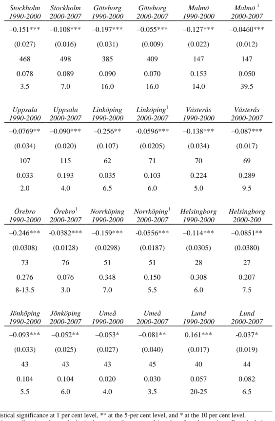
Table C1: Identification of municipality tipping points and results from regression discontinuity model for population changes around the tipping point (robust standard errors within parentheses)
Native population growth
Stockholm 1990-2000 Stockholm 2000-2007 Göteborg 1990-2000 Göteborg 2000-2007 Malmö 1990-2000 Malmö 1 2000-2007 Beyond Tipping Point –0.151*** –0.108*** –0.197*** –0.055*** –0.127*** –0.0460*** (0.027) (0.016) (0.031) (0.009) (0.022) (0.012) Number of observations 468 498 385 409 147 147 R-squared 0.078 0.089 0.090 0.070 0.153 0.050 Tipping Point % 3.5 7.0 16.0 16.0 14.0 39.5 Uppsala 1990-2000 Uppsala 2000-2007 Linköping 1990-2000 Linköping1 2000-2007 Västerås 1990-2000 Västerås 2000-2007 Beyond Tipping Point –0.0769** –0.090*** –0.256** -0.0596*** –0.138*** –0.087*** (0.034) (0.020) (0.107) (0.0205) (0.034) (0.017) Number of observations 107 115 62 71 70 69 R-squared 0.033 0.193 0.035 0.103 0.224 0.289 Tipping Point % 2.0 4.0 6.5 6.0 5.0 9.5 Örebro 1990-2000 Örebro1 2000-2007 Norrköping 1990-2000 Norrköping1 2000-2007 Helsingborg 1990-2000 Helsingborg 2000-200 Beyond Tipping Point –0.246*** -0.0382*** –0.159*** -0.0556*** –0.114*** –0.0851** (0.0308) (0.0128) (0.0298) (0.0187) (0.0305) (0.0380) Number of observations 73 76 51 51 28 27 R-squared 0.276 0.076 0.348 0.150 0.308 0.207 Tipping Point % 8-13.5 3.0 7.0 5.5 6.0 7.5 Jönköping 1990-2000 Jönköping 2000-2007 Umeå 1990-2000 Umeå 2000-2007 Lund 1990-2000 Lund 2000-2007 Beyond Tipping Point –0.093*** –0.052** –0.053* –0.081** 0.161*** -0.037* (0.033) (0.025) (0.027) (0.040) (0.017) (0.019) Number of observations 43 43 43 45 40 44 R-squared 0.104 0.104 0.020 0.030 0.057 0.082 Tipping Point % 5.5 6.0 4.0 3.5 20-25 6.5
Note: *** indicates statistical significance at 1 per cent level, ** at the 5-per cent level, and * at the 10 per cent level.
1
We have excluded obvious outliers in order to obtain tipping points that are not driven by a few observations. By calculating how much an observation influences the regression model as a whole (i.e. how much the predicted values change as a result of including and excluding a particular observation), SAMS areas with a |DfFIT| > 2*SQRT(k/N) were excluded. k is the number of parameters (including the intercept) and N is the sample size. In total, 12 observations were excluded due to having too large influence on the results.