Linköping Studies in Science and Technology Licentiate Thesis No. 1203
A model for simulation and generation of
surrounding vehicles in driving simulators
Johan Janson Olstam
LiU-TEK-LIC- 2005:58
Dept. of Science and Technology
Linköpings Universitet, SE-601 74 Norrköping, Sweden Norrköping 2005
A model for simulation and generation of surrounding vehicles in driving simulators
© 2005 Johan Janson Olstam johja@itn.liu.se
Department of Science and Technology Linköpings universitet, SE-601 74 Norrköping, Sweden. ISBN 91-85457-51-5 ISSN 0280-7971 LiU-TEK-LIC 2005:58
Acknowledgements
First of all I would like to thank my supervisors Jan Lundgren, Linköping University (LiU), Department of Science and Technology (ITN), and Pontus Matstoms, VTI, for their invaluable support and advices. Many thanks also to Mikael Adlers, VTI, who I have been working with during the integration and testing within the VTI Driving simulator III. He has a great part in that integration went successfully. Thanks also to the Swedish Road Administration (SRA), Ruggero Ceci, for funding this work.
I would also like to show appreciation to my other colleagues at ITN/LiU and VTI, whom make ITN/LiU and VTI stimulating places to work at. Special thanks to my roommate and PhD student colleague Andreas Tapani and to my other PhD student colleagues for very interesting and useful discussions, to Arne Carlsson, VTI, for sharing his knowledge within the traffic theory and simulation area, to Anne Bolling and Selina Mård Berggren, VTI, for their help during the design and the realization of the conducted driving simulator experiment, to Lena Nilsson and Jerker Sundström, VTI, for invaluable comments, and to the members of the VTI driving simulator group, Staffan, Mikael, Mats, Håkan, Håkan, and Göran, for sharing their massive experience within the driving simulator area.
I would also like to express my gratitude to my family and friends for their encouragement and support. Last but not least, I would like to give all my love to Lin and to my two cuddly cats Marion and Morriz.
Abstract
Driving simulators are used to conduct experiments on for example driver behavior, road design, and vehicle characteristics. The results of the experiments often depend on the traffic conditions. One example is the evaluation of cellular phones and how they affect driving behavior. It is clear that the ability to use phones when driving depends on traffic intensity and composition, and that realistic experiments in driving simulators therefore has to include surrounding traffic.
This thesis describes a model that generates and simulates surrounding vehicles for a driving simulator. The proposed model generates a traffic stream, corresponding to a given target flow and simulates realistic interactions between vehicles. The model is built on established techniques for time-driven microscopic simulation of traffic and uses an approach of only simulating the closest neighborhood of the driving simulator vehicle. In our model this closest neighborhood is divided into one inner region and two outer regions. Vehicles in the inner region are simulated according to advanced behavioral models while vehicles in the outer regions are updated according to a less time-consuming model. The presented work includes a new framework for generating and simulating vehicles within a moving area. It also includes the development of enhanced models for car-following and overtaking and a simple mesoscopic traffic model.
The developed model has been integrated and tested within the VTI Driving simulator III. A driving simulator experiment has been performed in order to check if the participants observe the behavior of the simulated vehicles as realistic or not. The results were promising but they also indicated that enhancements could be made. The model has also been validated on the number of vehicles that catches up with the driving simulator vehicle and vice versa. The agreement is good for active and passive catch-ups on rural roads and for passive catch-ups on freeways, but less good for active catch-ups on freeways.
Contents
1 INTRODUCTION ...1 1.1 BACKGROUND...1 1.2 AIM...3 1.3 DELIMITATIONS...3 1.4 THESIS OUTLINE...3 1.5 CONTRIBUTIONS...4 1.6 PUBLICATIONS...5 2 TRAFFIC SIMULATION ...72.1 CLASSIFICATION OF TRAFFIC SIMULATION MODELS...7
2.2 MICROSCOPIC TRAFFIC SIMULATION...8
2.3 BEHAVIORAL MODEL SURVEY...9
2.3.1 Car-following models ...10
2.3.2 Lane-changing models...16
2.3.3 Overtaking models ...22
2.3.4 Speed adaptation models ...25
3 SURROUNDING TRAFFIC IN DRIVING SIMULATORS ...27
3.1 DRIVING SIMULATOR EXPERIMENTS...27
3.1.1 Experiments, scenarios, and scenes...27
3.1.2 Design issues...28
3.2 USING STOCHASTIC TRAFFIC IN DRIVING SIMULATOR SCENARIOS...29
3.2.1 The stochastic traffic – Driving simulator dilemma ...29
3.2.2 Stochastic traffic simulation and critical events...30
3.3 DEMANDS ON TRAFFIC SIMULATION WHEN USED IN DRIVING SIMULATORS...31
3.4 RELATED RESEARCH...32
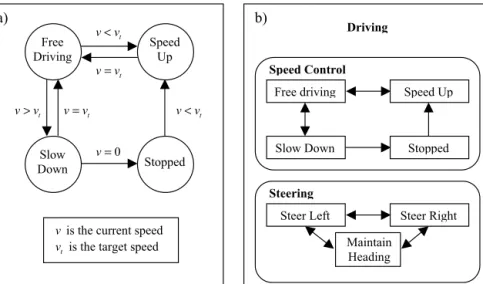
3.4.1 Rule-based models ...34
3.4.2 State machines ...35
3.4.3 The eco-resolution principle...36
4 THE SIMULATION MODEL...39
4.1 THE SIMULATION FRAMEWORK...39
4.1.1 Representation of vehicles and drivers...39
4.1.2 The moving window ...40
4.1.3 The simulated area...42
4.1.4 The candidate areas...42
4.1.5 Vehicle update technique ...45
4.2 VEHICLE GENERATION...48
4.2.1 Generation algorithm ...48
4.2.2 Generation of new vehicles on freeways...50
4.2.3 Generation of new vehicle and vehicle platoons on rural roads...53
4.2.4 Initialization of the simulation...54
4.3 BEHAVIORAL MODELS...55
4.3.1 Speed adaptation...55
4.3.2 Car-following...57
4.3.3 Lane-changing ...60
4.3.5 Passing...64
4.3.6 Oncoming avoidance ...64
5 INTEGRATION WITH THE VTI DRIVING SIMULATOR III...67
5.1 THE VTI DRIVING SIMULATOR III ...67
5.2 THE INTEGRATED SYSTEM...67
5.3 COMMUNICATION WITH THE SCENARIO MODULE...68
6 VALIDATION ...71
6.1 HOW SHOULD THE MODEL BE VALIDATED?...71
6.2 NUMBERS OF ACTIVE AND PASSIVE OVERTAKINGS...72
6.2.1 Simulation design...73 6.2.2 Results...74 6.3 USER EVALUATION...79 6.3.1 Experimental design ...79 6.3.2 Scenario design...80 6.3.3 Evaluation design ...81
6.3.4 Results and analyses of the questionnaire ...82
6.3.5 Results and analyses of the interview questions ...83
6.4 DISCUSSION...86
6.4.1 Some additional observations...87
7 CONCLUSIONS AND FUTURE RESEARCH...89
8 REFERENCES...91
Appendices
APPENDIX A – DRIVER/VEHICLE PARAMETER VALUES APPENDIX B – OVERTAKING PARAMETERS
APPENDIX C – QUESTIONNAIRE
APPENDIX D – INTERVIEW QUESTIONS
1 Introduction
1.1 Background
Traffic safety is a severe and important problem. Many accidents are caused by failures in the interaction between the driver, the vehicle, and the traffic system. The number of driving related interactions is increasing. Drivers nowadays also interact with different intelligent transportation systems (ITS), advanced driver assistance systems (ADAS), in-vehicle information systems (IVIS), and NOMAD devices, such as mobile phones, personal digital assistants, and portable computers. These technical systems influence drivers’ behavior and their ability to drive a vehicle. To be able to evaluate how different ITS, ADAS, IVIS, NOMAD-systems, or road and signal control designs etc influence drivers, knowledge about the interactions between drivers, vehicles and environment are essential.
To get this knowledge researchers conduct behavioral studies and experiments, which either can be conducted in the real traffic system, on a test track, or in a driving simulator. The real world is of course the most realistic environment, but it can be unpredictable regarding for instance weather-, road- and traffic conditions. It is therefore often hard to design real world experiments from which it is possible to draw statistically significant conclusions. Some experiments are also too dangerous or expensive to conduct in the real world and other are impossible due to laws or ethical reasons. Test tracks offer a safer environment and the possibility of giving test drivers more equal conditions and thereby decreasing the statically uncertainty. However, test tracks lack a lot in realism and it can be hard to evaluate how valid results from a test track study are for driving on a real road. Driving simulators on the other hand offer a realistic environment in which test conditions can be controlled and varied in a safe way.
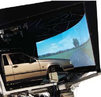
A driving simulator is designed to imitate driving a real vehicle, see Figure 1.1 for an illustration. The driver place can be realized with a real vehicle cabin or only a seat with a steering wheel and pedals, and anything in between. The surroundings are presented for the driver on a screen. A vehicle model is used to calculate the simulator vehicle’s movements according to the driver’s use of the steering wheel and the pedals. Some driving simulators use a motion system in order to support the driver’s visual impression of the simulator vehicle’s movements. Last but not least a driving simulator include a scenario module that includes the specification of the road, the environment, and all other actors and events.
Figure 1.1 The VTI Driving Simulator III (Source: Swedish National Road and
Transport Research Institute (VTI) (2004))
Driving simulators are used to conduct experiments in many different areas such as:
• Alcohol, medicines and drugs. • Driving with disabilities.
• Technical systems, such as ITS, ADAS, IVIS, and NOMAD systems. • Fatigue
• Road design • Vehicle design
Driving simulators can also be used for training purposes. One example is the TRAINER simulator that was developed to work as a complimentary vehicle in driving license schools, (Gregersen et al., 2001). The TRAINER simulator offers great possibilities to train actions that are unsafe, difficult or impossible to train in the real road network. This could be anything between basic maneuvering to emergency situations.
It is important that the performance of the simulator vehicle, the visual representation, and the behavior of surrounding objects are realistic in order for the driving simulator to be a valid representation of real driving. It is for instance clear that the ambient vehicles must behave in a realistic and trustworthy way. Ambient vehicles influence the driver’s mental load and thereby his or her ability to drive the vehicle. A good representation of the ambient vehicles is especially important in simulator studies where the traffic intensity and composition has a large impact on the driver’s ability to drive the vehicle. This can for instance be in experiments concerning road design, the use of new technical equipment, or fatigue. It is not only important that the behavior of a single driver is realistic, but
also that the behavior of the whole traffic stream is realistic. For instance, drivers who drive fast expect to catch up with more vehicles than catches up with them and vice versa.
A realistic simulation of surrounding vehicles, and thereby traffic, can be achieved by combining a driving simulator with a model for microscopic simulation of traffic. Micro-simulation has become a very popular and useful tool in studies of traffic systems. Micro models use different sub-models for car-following, lane-changing, speed adaptation, etc. to simulate driver behavior at a microscopic level. The sub-models, hereby called behavioral models, use the current road and traffic situation as inputs and generates individual driver’s decisions regarding for example which acceleration to apply and which lane to travel in as outputs. Stochastic functions are often used to model variation in driver behavior, both among drivers and over time for a specific driver. However, stochastic traffic simulation models have traditionally not been used to simulate ambient vehicles in driving simulators. The usual approach has instead been to simulate the ambient vehicles according to deterministic models. There are for several reasons desirable to keep the variation in test conditions between different drivers as low as possible. By using stochastic simulation of ambient traffic, drivers will experience different situations at the micro level depending on how they drive. The simulator driver’s conditions will still be comparable at a higher, more aggregated, level, if this is sufficient or not varies depending on the type of experiment. For some experiments, equal conditions at the micro level are essential and stochastic simulation may not be suitable to use. In other experiments, comparable conditions at a higher level are sufficient.
1.2 Aim
The aim of this thesis is to develop, implement, and validate a real-time running traffic simulation model that is able to generate and simulate surrounding vehicles in a driving simulator. This includes integration of the developed model and a driving simulator. The model should both simulate individual vehicle-driver units and the traffic stream that they are a part of, in a realistic way. The simulated vehicle-driver units should behave realistically concerning acceleration, lane-changing, and overtaking behavior, as well as concerning speed choices. The vehicles should also appear in the traffic stream in such a way that headways, vehicle types, speed distributions, etc. correspond to real data.
1.3 Delimitations
The simulation model has been delimited to only deal with freeways with two lanes in each direction and to rural roads with oncoming traffic. The model does not deal with ramps on freeways or intersections on rural roads. Consequently, the thesis does not deal with simulation of urban traffic situations.
Some driving simulator experiments include critical situations or events. To create such situations autonomous vehicles has to be combined with vehicles with predetermined behavior. The thesis only discusses this topic to a limited extent.
1.4 Thesis outline
Chapter 2 gives an introduction to the field of microscopic simulation of traffic. The chapter includes a survey of common car-following, lane-changing, overtaking, and speed adaptation models.
Chapter 3 includes an introduction to driving simulator experiments and to the field of simulation of surrounding vehicles in driving simulators. It also include a discussion on the advantages, disadvantages, and difficulties of using stochastic traffic simulation for simulating surrounding vehicles in driving simulators. The chapter ends with a description of related research.
In Chapter 4 the proposed model is presented. First, the simulation framework is presented. Then follows the presentation of the technique used to generate new vehicles. The chapter ends with a description of the utilized behavioral models and calibration of the involved parameters.
Chapter 5 describes the integration of the proposed simulation model and the VTI driving simulator III. The chapter starts with a short description of the driving simulator and then follows the description of the integrated system.
The performed validation of the model is presented in Chapter 6. The chapter starts with a discussion on how to validate this kind of models. Then follows a description and results from a validation of the number of vehicles that catches up with the driving simulator vehicle and vice versa. The third section describes a driving simulator experiment that was conducted in order to validate the simulated vehicles’ behavior. The chapter ends with a discussion and some additional observations made during tests in the driving simulator.
Chapter 7 ends the thesis with a summary and a discussion on future research needs and possibilities.
1.5 Contributions
The main contribution of this thesis is the developed traffic simulation model, which is able to simulate ambient vehicles in a driving simulator on freeways and on rural roads with oncoming traffic. The contributions also include:
• A summary over commonly used behavioral models for car-following, lane-changing, overtaking, and speed adaptation.
• An investigation of difficulties, benefits, advantages and disadvantages with using stochastic micro simulation of traffic for simulation of ambient traffic in a driving simulator.
• Improvements of a technique for generating freeway traffic on a moving area around a driving simulator and a further development of this technique to also fit generation of vehicles on rural roads without a barrier between oncoming traffic.
• A new simple mesoscopic traffic simulation model that simulates individual vehicles using speed-flow diagrams. The model is used to simulate vehicles far away from the simulator vehicle.
• A new version of the TPMA (Davidsson et al., 2002) car-following model, including a new deceleration model.
• An enhanced version of the VTISim (Brodin et al., 1986) overtaking model, which includes new models for the behavior during the overtaking and at abortion of overtakings.
• Integration of the simulation model and the VTI Driving simulator III • Presentation of different approaches that can be used to validate models
1.6 Publications
Some parts of this thesis have been published in other publications. The first version of the framework for generation and simulation of vehicles on freeways was originally presented in
Janson Olstam, J. and J. Simonsson (2003), Simulerad trafik till VTI:s körsimulator - en förstudie (Simulated traffic for the VTI driving simulator - a feasibility study, In Swedish). VTI Notat 32-2003. Swedish National Road and Transport Research Institute (VTI), Linköping, Sweden.
A partly enhanced version of this framework was later presented in
Janson Olstam, J. (2003). “Traffic Generation for the VTI Driving Simulator”. In Proceedings of: Driving Simulator Conference - North America, DSC-NA 2003, Dearborn, Michigan, USA.
The generation and simulation framework for simulation of rural road traffic for driving simulators was first presented in:
Janson Olstam, J. (2005). “Simulation of rural road traffic for driving simulators”. In Proceedings of: 84th Annual meeting of the Transportation Research Board, Washington D.C., USA.
Section 2.3.1 in the thesis includes a survey over car-following models. The main part of this survey has been presented in:
Janson Olstam, J. and A. Tapani (2004), Comparison of Car-following models. VTI meddelande 960A and LiTH-ITN-R-2004-5. Swedish National Road and Transport Research Institute (VTI) and Linköping University, Department of Science and Technology, Linköping, Sweden.
2 Traffic simulation
The societies of today need well working traffic and transportation systems. Congestion and traffic jams have become recurrent problems in most of the larger cities and also more common in smaller cities. In order to avoid congestion and to optimize the traffic systems with respect to capacity, accessibility and safety, traffic planners need tools that can predict the effects of different road designs, management strategies, and increased travel demands. Researchers and developers have therefore during the last decades developed many different types of models and tools that deal with these kinds of issues. The rapid development in the personal computer area has created new possibilities to develop enhanced traffic modeling tools. Traffic models are mainly based on analytical or simulation approaches. The analytical models often use queue theory, optimization theory or differential equations that can be solved analytical to model road traffic. These kinds of models are very useful, but often lack the possibility of studying how the dynamics of a traffic system varies over time. Simulation models on the other hand offer this possibility. They model how the traffic changes over time and use stochastic functions in order to reproduce the dynamics of a traffic system.
Traffic simulation has become a powerful and cost-efficient tool for investigating traffic systems. It can for instance be used for evaluation of different road and regulation designs, ITS-applications or traffic management strategies. Traffic simulation models offer the possibility to experiment in a safe and non-disturbing way with an existing or non-existing traffic system. As all models, traffic simulation models must be calibrated and validated in order to generate trustworthy results. This is often a very time-consuming task and sometimes limits the models cost-efficiency.
2.1 Classification of traffic simulation models
There are many different kinds of traffic models and there are also a couple of different ways to classify traffic models. Traffic simulation models are typical classified according to the level of detail at which they represent the traffic stream. Three categories are generally used, namely: Microscopic, Mesoscopic and Macroscopic.
Microscopic models represent the traffic stream at a very high level of detail. They model individual vehicles and the interaction between them. Microscopic models incorporate sub-models for acceleration, speed adaptation, lane-changing, gap acceptance etc., to describe how vehicles move and interact with each other and with the infrastructure. Several models have been developed and the most well-known are probably AIMSUN (Barceló et al., 2002), VISSIM (PTV, 2003), Paramics (Quadstone, 2004a, Quadstone, 2004b), MITSIMLab (Toledo et al., 2003), and CORSIM (FHWA, 1996).
Mesoscopic models often represent the traffic stream at a rather high level of detail, either by individual vehicles or packets of vehicles. The difference compared to micro models is that interactions are modeled with lower detail. The interactions between vehicles and the infrastructure are typically based on macroscopic relationships between, for example, flow, speed and density. Examples of mesoscopic simulation models are DYNASMART (Jayakrishnan et al., 1994) and CONTRAM (Taylor, 2003).
Macroscopic models use a low level of detail, both regarding the representation of the traffic stream and interactions. Instead of modeling individual vehicles, the
macro models use aggregated variables as flow, speed and density to characterize the traffic stream. Macro models commonly use speed-flow relationships and conservation equations to model how traffic propagate thru the modeled network. Examples of macroscopic simulation models are METANET/METACOR (Papageorgiou et al., 1989, Salem et al., 1994) and the Cell Transmission model (Daganzo, 1994, Daganzo, 1995).
2.2 Microscopic traffic simulation
Microscopic traffic simulation models, hereby called micro or traffic simulation models, simulate individual vehicles. The general approach is to treat a driver and a vehicle as one unit. As in reality, these vehicle-driver units interact with each other and with the surrounding infrastructure. Micro models consist of several sub-models, hereby called behavioral models, that each handles specific interactions. The most essential behavioral model is the car-following model, which handles the longitudinal interaction between two preceding vehicles. Other important behavioral models include models for lane-changing, gap-acceptance, overtaking, ramp merging, and speed adaptation. The sub-models needed depend on which type of road that the model should be able to simulate. Lane-changing models are for instance only necessary when simulating urban or freeway environments and are not needed in models for two lane highways without a barrier between oncoming lanes. The most common behavioral models will be presented in more detail in Section 2.3.
Most micro models are able to simulate urban or freeway networks. The most well known models for these environments are also the ones presented in Section 2.1 (AIMSUN, VISSIM, Paramics, MITSIMLab, and CORSIM). Only a couple of models for two-lane highways with oncoming traffic have been developed. The state-of-the-art in rural road models includes the Two-Lane Passing (TWOPAS) model (Leiman et al., 1998), the Traffic on Rural Roads (TRARR) model (Hoban et al., 1991), and the VTISim model (Brodin et al., 1986). The VTISim model is currently being further developed in the Rural Road Traffic Simulator (RuTSim) model (Tapani, 2005).
In order to model that behavior and preferences varies among drivers, each vehicle driver unit is assigned different driver characteristics parameters. These parameters commonly include vehicle length, desired speed, desired following distance, possible or desired acceleration and deceleration rates, etc. The variation among the population is generally described by a distribution function and individual parameter values are drawn from the specified distribution. We can for example assume that desired speeds on freeways follows a normal distribution with mean 111 km/h and a standard deviation of 11 km/h.
Micro models are generally time-discrete, but some event based models has also been developed, see for instance Brodin and Carlsson (1986). The basic principle of a time discrete model is that time is divided into small time steps, commonly between 0.1 and 1 second. At each time step the model updates every vehicle according to the set of behavioral models. At the end of the time step the simulation clock is increased and the simulation enters the next time step.
Microscopic simulation models have traditionally been used to perform capacity and level-of-service evaluations of different road designs and management strategies. During the last decade, micro models have also in greater extent been used to evaluate different ITS-applications for example Intelligent
Speed Adaptation (Liu et al., 2000) or Adaptive Cruise Control systems (Champion et al., 2001). Research has also been made within in the area of combining micro simulation and different safety indicators to perform safety analysis of different road and intersection designs, see for example Archer (2005) and Gettman et al. (2003).
Even though micro models work on a micro level and simulate individual vehicles, they have mainly been used to generate macroscopic outputs such as average speeds, flows, and travel times. A large part of the calibration and validation of micro models are therefore generally performed at a macroscopic level. The different behavioral model has to various extents been calibrated and validated at a micro level. However, very little effort has been put into calibrating and validating combinations of behavioral models at a micro level, for example if a car-following model in combination with a lane-changing model generates valid results at a micro level.
2.3 Behavioral model survey
In order to be usable and well performing, traffic simulation models must be based on high-quality behavioral models. To generate realistic behavior is of course the most important property of a good behavioral model, but not the only desirable property. A very realistic behavioral model is of little or no use if it cannot be calibrated or if this task is too time-consuming. It is therefore desirable to keep the number of model parameters as low as possible. When designing a behavioral model the aim should be to find the best compromise between the number of parameters and output agreement. It is also desirable that the utilized parameters easily can be interpreted as known vehicle or driver factors. This simplifies the calibration work and allows the user to in a more straightforward and easy way experiment with different parameter settings regarding for example the variation in behavior among drivers.
Different road environments require different kinds of behavioral models. A traffic simulation model for urban roads must include different types of behavioral models compared to a simulation model for rural environments. Common for all environments is however the need of a car-following model. A car-following model controls drivers’ acceleration behavior with respect to the preceding vehicle in the same lane. It deduce when a vehicle is free or following a preceding vehicle and what action to take in each case. Another behavioral model necessary in all road environments is a speed adaptation model, which calculates a driver’s preferred or desired speed along the road. In urban and freeway environments, models for lane-changing decisions are essential. However, on two-lane highways a model that consider the whole overtaking procedure is needed. Such a model cannot only deal with the lane change to the oncoming lane. It also has to consider the actual passing procedure when traveling in the oncoming lane and the lane change back to the own lane. As a part of both lane-changing and overtaking models some type of gap-acceptance model is necessary. A Gap-acceptance model controls the decision of accepting or rejecting an available gap, for example if a vehicle that wants to change lane accept the available gap between two subsequent vehicles in the target lane. Some kind of gap-acceptance model is also necessary when modeling intersections, lane drops or on-ramp weaving decisions. The following sections will describe different kinds of car-following, lane-changing, overtaking, and speed adaptation models in more detail. The sections
also include descriptions of different approaches to gap-acceptance in connection to lane-changes and overtakings.
2.3.1 Car-following models
A car-following model controls driver’s behavior with respect to the preceding vehicle in the same lane. A vehicle is classified as following when it is constrained by a preceding vehicle, and driving at the desired speed will lead to a collision. When a vehicle is not constrained by another vehicle it is considered free and travels, in general, at its desired speed. The follower’s actions is commonly specified through the follower’s acceleration, although some models, for example the car-following model presented in Gipps (1981), specify the follower’s actions through the follower’s speed. Some car-following models only describe drivers’ behavior when actually following another vehicle, whereas other models are more complete and determine the behavior in all situations. In the end, a car-following model should deduce both in which regime or state a vehicle is in and what actions it applies in each state. Most car-following models use several regimes to describe the follower’s behavior. A common setup is to use three regimes: one for free driving, one for normal following, and one for emergency deceleration. Vehicles in the free regime are unconstrained and try to achieve their desired speed, whereas vehicles in the following regime adjust their speed with respect to the vehicle in front. Vehicles in the emergency deceleration regime decelerate to avoid a collision. The following notation will be used throughout this section to describe the car-following models, see also Figure 2.1:
n a Acceleration, vehicle n , [m/s2] n x Position, vehicle n , [m] n v Speed, vehicle n , [m/s] x ∆ xn−1−xn, space headway, [m] v ∆ vn−vn−1, difference in speed, [m/s] desired n
v Desired speed, vehicle n , [m/s]
1
n
L − Length, vehicle n -1, [m] 1
n
s − Effective length (Ln−1+ minimum gap between stationary vehicles),
vehicle n -1, [m] T Reaction time, [s]
Figure 2.1 Car- following notation.
n n-1 n x 1 n x− 1 n L− Direction
Classification of car-following models
Car-following models are commonly divided into classes or types depending on the utilized logic. The Gazis-Herman-Rothery (GHR) family of models is probably the most studied model class. The GHR model is sometimes referred to as the general car-following model. The first version was presented in 1958 (Chandler et al., 1958) and several enhanced versions have been presented since then. The GHR model only controls the actual following behavior. The basic relationship between a leader and a follower vehicle is in this case a stimulus-response type of function. The GHR model states that the follower’s acceleration depends on the speed of the follower, the speed difference between follower and leader, and the space headway (Brackstone et al., 1998). That is, the acceleration of the follower at time t is calculated as
( ) ( ) ( ( ) ( )) ( ) ( ) ( ) 1 1 n n n n n n v t T v t T a t v t x t T x t T β γ α − − − − − = ⋅ ⋅ − − − , (2.1)
where α > , β and γ are model parameters that control the proportionalities. A 0 GHR model can be symmetrical or unsymmetrical. A symmetrical model uses the same parameter values in both acceleration and deceleration situations, whereas an unsymmetrical model uses different parameter values in acceleration and deceleration situations. An unsymmetrical GHR-model is for instance used in MITSIM (Yang et al., 1996) to calculate the acceleration in the following regime, and is formulated as ( ) ( ) ( ( ) ( )) ( ) ( ) ( ) 1 1 1 n n n n n n n v t T v t T a t T v t x t T l x t T β γ α± ± − ± − − − − − − = ⋅ ⋅ − − − − (2.2)
where α±, β± and γ± are model parameters. The parameters α+, β+and γ+
are used if vn ≤vn−1and α−, β−and γ− are used if vn >vn−1. Besides the
following regime, the MITSIM model uses one emergency regime and a free driving regime.
The safety distance or collision avoidance models constitute another type of car-following model. In these models, the driver of the following vehicle is assumed to always try to keep a safe distance to the vehicle in front. Pipes’ rule which says: “A good rule for following another vehicle at a safe distance is to allow yourself at least the length of a car between you and the vehicle ahead for every ten miles of hour speed at which you are traveling”, (Hoogendoorn et al., 2001), is a simple example of a safety distance model. The safe distance is however commonly specified through manipulations of Newton’s equations of motion. In some models, this distance is calculated as the distance that is necessary to avoid a collision if the leader decelerates heavily. The most well known safety distance model is probably the one presented in Gipps (1981). In this model the follower choose the minimum speed of the one constrained by the own vehicle and the one constrained by the leader vehicle, that is the minimum of
( ) ( ) 2.5 m 1 n( ) 0.025 n( ) a n n n desired desired n n v t v t v t T v t a T v v + = + ⋅ ⋅ ⋅ − ⋅ + (2.3) and ( ) ( ) ( ( ) ) ( ) ( ) 2 2 1 m m m 1 1 2 nˆ b n n n n n n n v t v t T d T d T d x t s v t T d − − − + = + − ∆ − − − (2.4) Here m n a and m n
d is the maximum desired acceleration and deceleration for vehicle n, respectively, and dˆn−1 is an estimation of the maximum deceleration desired by
vehicle n-1. The safe speed with respect to the leader (equation (2.4)) is derived from the Newtonian equations of motion. The equation calculates the maximum speed that the follower can drive at and still be able to, after some reaction time, decelerate down to zero speed and avoid a collision if the leader decelerates down to zero speed.
In 1963 a new approach for car-following modeling were presented, (Brackstone et al., 1998). Models using this approach are classified as psycho-physical or action point models. The GHR models assume that the follower reacts to arbitrarily small changes in the relative speed. GHR models also assume that the follower reacts to actions of its leader even though the distance to the leader is very large and that the follower’s response disappears as soon as the relative speed is zero. This can be corrected by either extending the GHR-model with additional regimes, e.g. free driving and emergency deceleration, or using a psycho-physical model. Psycho-physical models use thresholds or action points where the driver changes his or her behavior. Drivers are able to react to changes in spacing or relative velocity only when these thresholds are reached, (Leutzbach, 1988). The thresholds, and the regimes they define, are often presented in a relative space/speed diagram of a follower – leader vehicle pair; see Figure 2.2 for an example. The bold line symbolizes a possible vehicle trajectory.
Figure 2.2 A psycho-physical car-following model (Source: (Leutzbach, 1988)).
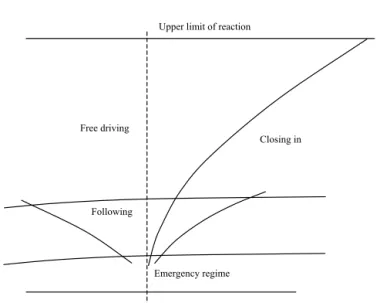
Representative examples of psycho-physical car-following models are the ones presented in Wiedemann and Reiter (1992), see Figure 2.3, and Fritzsche (1994), see Figure 2.4.
Figure 2.3 The different thresholds and regimes in the Wiedemann car-following
model.
Emergency regime Following
Upper limit of reaction
0 Free driving Closing in v ∆ x ∆ Zone without reaction 0 ∆v x ∆ Zone with reaction Zone with reaction Vehicle trajectory
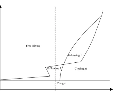
Figure 2.4 The different thresholds and regimes in the Fritzsche car-following
model.
Fuzzy-logic is another approach that to some extent has been utilized in car-following modeling. Fuzzy logic or fuzzy set theory can be used to model drivers inability to observe absolute values. Human beings cannot observe exact values of for instance speed or relative distance, but they can give estimations like “above normal speed”, “fast”, “close”, etc. In the earlier described models drivers are assumed to know their exact speed and distance to other vehicles etc. In order to get a more human-like modeling, fuzzy logic models assume that drivers only are able to conclude, for example, if the speed of the front vehicle is very low, low, moderate, high, or very high. In many cases the fuzzy sets overlap each other. To deduce how a driver will observe a current variable value, membership functions that map actual values to linguist values has to be specified, see Figure 2.5 for an example.
Figure 2.5 Example of membership functions for driving speed
The strength with fuzzy logic is that the fuzzy sets easily can be combined with logical rules to different kinds of behavioral models. A possible rule can for
speed
low moderate very high
0 1 high very low Membership value Following II Following I Closing in Free driving 0 ∆v x ∆ Danger
“large” then increase speed. As seen in the previous sentence, it is rather easy to create realistic and workable linguistic rules for a specific driving task. However, one big problem is that the fuzzy sets need to be calibrated in some way. There have been attempts to “fuzzify” both the GHR model and a model named MISSION (Wiedemann and Reiter, 1992). However, no attempts to calibrate the fuzzy sets have been made, (Brackstone and McDonald, 1998).
Model properties
As presented in the previous section, there are different types of car-following models. Several car-following models, with varying approaches, have been developed since the 1950’s. Despite the number of already developed models, there is still active research in the area. One reason for this is that the preferred choice of car-following model may differ depending on the application. For example, the requirements placed on a car-following model used to generate macroscopic outputs, e.g. average flow and speed, is lower than the requirements on car-following models used to generate microscopic output values, such as individual speed and position changes.
Traffic simulation and thereby car-following models are mostly utilized to study how changes in a network affect traffic measures such as average flow, speed, density etc. The simulation output of interest in such applications are in other words macroscopic measures, hence the utilized car-following models should at least generate representative macroscopic results. Leutzbach (1988) presents a macroscopic verification of GHR-models. Through integration of the car-following equation it is possible to obtain a relation between average speed, flow and density. This relationship can then be compared to real data or to outputs from other macroscopic models. For a GHR-model with β = and 0 γ= the 2 integration arrives at the well recognized Greenshields relationship (see for example May (1990)): max 1 desired k q v k v k k = ⋅ = ⋅ − ⋅ , (2.5)
where q is the traffic flow (vehicles/hour), k is the density (vehicles/km) and
max
k is the maximal possible density (jam density). A verification of this kind is however not possible for an arbitrary car-following model. It is for example not possible to integrate a psycho-physical model, since such models don’t express the follower’s acceleration in mathematically closed form. Macroscopic relationships can however always be generated by running several simulations with different flows.
Drivers’ reaction time is a parameter common in most car-following models. It is assumed that with very long reaction times, vehicles have to drive with large gaps between each other in order to avoid collisions, hence the density, and thereby the flow, will be reduced. Most car-following models use one common reaction time for all drivers. This is not very realistic from a micro perspective but may be enough to generate realistic macro results.
The magnitude of drivers’ reactions also influences the result. How the output is affected is not as obvious as in the reaction time case. High acceleration rates should lead to that vehicles reach their new constraint speed faster, which would
decrease the vehicles travel time delay. High deceleration rates should also lead to less travel time delay, thus the vehicles can start their decelerations later. High acceleration and retardation rates may however result in oscillating vehicle trajectories at congested situations and thereby decrease the average speed.
Car-following models utilized in applications where microscopic output data is required must of course generate driving behavior as close as possible to real driving behavior. This is the case in simulation of surrounding traffic for a driving simulator or simulation used to estimate exhaust pollution, which requires detailed information about the vehicles’ driving course of events. One should however bear in mind that the calibration of models used to produce microscopic output is considerably more expensive than the calibration of models used to estimate macroscopic traffic measures.
There are many possible pitfalls in the modeling of car-following behavior. Firstly, driver parameters such as reaction time and reaction magnitude vary among drivers. The behavior may also differ between different countries or territories, due to different formal and informal driving and traffic rules. Drivers in the USA may, for example, not drive in the same way as European or Asian drivers. Car-following models that is used to model traffic in different countries must therefore offer the possibility to use different parameter settings. The differences between countries may however be so big that the same car-following model cannot be used even with different parameter values to describe the behavior in two countries with very different traffic conditions.
Further more, it may be necessary to use different parameters, or even different models, for different traffic situations, for example congested and non-congested traffic. There are versions of the GHR model that use different parameter values at congested and non-congested situations, (Brackstone et al., 1998). The reaction time may, for example, vary for one driver depending on traffic situation. Drivers may be more alert at congested situations and thereby have a shorter reaction time than in non-congested situations.
Modeling of congested situations and the transition from normal non-congested traffic to a congested state also place additional requirements on the car-following modeling. If the model is to give a correct description of the jam build up and the capacity drop in these situations the car-following model must yield higher queue inflows than queue discharge rates, (Hoogendoorn et al., 2001).
2.3.2 Lane-changing models
Lane-changing models describe drivers’ behavior when deciding whether to change lane or not on a multi-lane road link. This type of behavioral model is essential and very important both in urban and freeway environments. When deciding whether to change lane, a driver need to consider several aspects. Gipps (1986) proposed that a lane-changing decision is the result of answering the questions
• Is it necessary to change lanes? • Is it desirable to change lanes? • Is it possible to change lanes?
Gipps (1986) presented a framework for the structure of lane-changing decisions in form of a decision tree. The proposed decision tree considered, in addition to
the list above, the driver’s intended turn, any reserved lanes or obstructions, and the urgency of the lane change in terms of the distance to the intended turn. Several lane-changing models such as (Barceló et al., 2002, Hidas, 2002, Yang, 1997) are based on the three basic steps proposed in Gipps (1986).
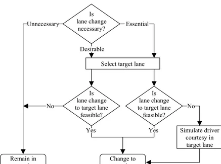
In the Gipps (1986) model all lane changes are impossible if the available gap in the target lane is smaller than a given limit. This is a reasonable approach in cases where a lane change is desirable. However, in situations where a lane change is necessary or essential but not possible, vehicles in the target lane often helps the trapped vehicle by decreasing its speed and creating a large enough gap for the trapped vehicle to enter. This has for instance been pointed out in Hidas (2002). Hidas (2002) describes a further developed variant of the model presented in Gipps (1986), which also includes the cooperative behavior for vehicles in the target lane, see Figure 2.6.
Figure 2.6 Structure for lane-changing decisions proposed in Hidas (2002).
An enhanced variant of this model has later been presented in Hidas (2005). In the Hidas (2002) structure the necessary and desirable steps are merged into one necessary step with the possible outcomes: unnecessary, desirable, or essential. A similar approach for modeling cooperative lane-changing has been presented in Yang and Koutsopoulos (1996). This model classifies a lane change as either mandatory or discretionary. Mandatory lane changes corresponds to the essential statement in Hidas (2002), that is lane changes necessary in order to pass lane blockage, reach an intended turn, avoid restricted lanes, etc. Discretionary lane changes refers to lane changes in order to gain speed advantages, avoid lanes close to on-ramps, etc, which can be compared to the desirable path in the Hidas (2002) structure. In both structures, the differences between mandatory and discretionary lane changes is in the gap-acceptance behavior and the possibility
Is lane change necessary? Is lane change to target lane feasible? Is lane change to target lane feasible? Select target lane
Simulate driver courtesy in target lane Change to target lane Remain in current lane Unnecessary Essential Desirable Yes No Yes No
that vehicles in the target lane may renounce their right of way in favor for a vehicle performing a mandatory lane change.
Toledo et al. (2005) pointed out that in principle all lane-changing models only consider lane changes to an adjacent lane. The models evaluate whether the driver should change to an adjacent lane or stay in the current one. Thus, most models lack an explicit tactical choice regarding their lane-changing behavior. Toledo et al. (2005) presented a model in which a driver chooses a target lane, not necessary an adjacent lane, that is most beneficial for the driver. In this way the driver will strive for reaching the most beneficial lane, which may need several lane changes to reach. This model follows in principle the basic decision structure proposed in Gipps (1986). However, the necessary and desired steps are merged into one target lane choice. This is possible since lanes that are less convenient, due to for example the next turning movement, will be less beneficial for the driver. In Toledo et al. (2005) a utility function is used to calculate the benefit of each lane and a discrete choice model is used to model the lane choice. This model will be described in more detail later on in this section when discussing the drivers desire to change lane.
El hadouaj et al. (2000) proposed a similar model as Toledo et al. (2005) in which drivers not only base their lane-changing decisions on the traffic situation in their own and one adjacent lane. Instead, the simulated drivers base their lane changes on the situations in all lanes. The model does not only consider the traffic situation in the closest area around the driver but do also account for the situation further away. The area around a driver is divided into several, in the paper 20, different areas. Lane changes are then based on the benefits in the different areas. This benefit is calculated through an assessment function that considers the speed and stability in the different areas around the driver. The model is based on psychological driver behavior studies performed at the French research institute INRETS and the Driving Psychology Laboratory (LPC), (El hadouaj et al., 2000). Modeling the urgency to change lane
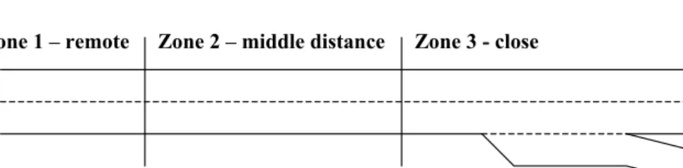
The urgency or necessity to change lane depends very much on the distance to an obstacle or an intended turn. This can and has been modeled in a couple of different ways. Gipps (1986) used three different areas, close, middle distance, and remote, defined by two time distances to the intended turn or obstacle, see Figure 2.7 for an example.
Figure 2.7 The three different lane-changing zones proposed by Gipps (1986)
After trials, suitable values of 10 s and 50 s for the two headways were proposed, (Gipps, 1986). This zone division has later been adopted and further developed in both Hidas (2002) and Barceló and Casas (2002). A similar zone division has also
Zone 3 - close Zone 2 – middle distance
Zone 1 – remote
considered far away from its intended turning or any obstacle and change lane if it desire. A vehicle in zone 2 is closer to its intended turn and is assumed to be a little bit more restrictive in its lane changing decisions. Vehicles in zone 2 do often not change to lanes further away from the lane suitable for the next turning. In zone 3, all lane-changing decisions exclusively focus on getting into the suitable lane. A vehicle in zone 3 that do not travel in the suitable lane for its intended turning will get more aggressive and start to accept smaller gaps. This will be discussed further on under the sub-section Gap-acceptance.
Yang (1997) proposed another way of modeling the drivers urgency to change lane. Instead of using different zones, vehicles are tagged to mandatory state according to a probability function. In Yang (1997) an exponential probability function were used, in which the probability to tag a vehicle as mandatory mainly depends on the distance to the intended turning or obstacle. This strategy has also been adopted in Wright (2000), but the exponential distribution were replaced with a linear relationship in order to save computational time.
Modeling drivers’ desire to change lane
The drivers desire to change lane can be modeled in several ways, for example by using
• A car-following model • A pressure function • Discrete choice theory • Fuzzy logic
In the model proposed in Gipps (1986) a car-following model, more precisely the model presented in Gipps (1981) (see equation (2.3) and (2.4)), was used to calculate which lane that has the least effect on the drivers speed. The model also accounted for the presence of heavy vehicles in the different lanes by calculating the effect of the next heavy vehicle in each lane as if they were the just preceding vehicles in respective lane. The model in Gipps (1986) also includes a relative speed condition for deciding if a driver is willing to change lane. As default values 1 m/s and -0.1 m/s were used for lane changes towards the centre and the curb, respectively, i.e. vehicles do not intend to change lane to the left if they are not driving 1 m/s faster then the preceding vehicle in the current lane.
A similar variant of using the car-following model to evaluate which lane that is most preferable has been presented in Kosonen (1999). Instead of using the car-following model, a pressure function was defined. This pressure function is an approximation of the potential deceleration rate caused by the leading vehicle and is defined as ( )2 2 des obs v v P s − = ⋅ , (2.6)
where vdes is the desired speed, vobs is the obstacle’s speed, and s is the relative
distance. The pressure function is used to model drivers lane-changing decision according to the logic described in Figure 2.8.
Figure 2.8 The lane-changing logic proposed by Kosonen (1999). P is calculated
according to equation (2.6). The parameters c and l c are calibration r
parameters, which controls the willingness to change to the left and right, respectively.
The logic is combined with a minimum time before a new lane change constraint in order to avoid to frequent lane-changing behavior. For lane changes to the left it is also combined with a minimum difference in desired speed condition, similar to the one used in Gipps (1986).
Toledo et al (2005) presented a model in which the necessary and desired step is merged together into a target lane model. The model is based on discrete choice theory and calculates the benefit of each lane using the utility function
{ }
int int int lane 1, lane 2, ...
T
TL TL TL TL TL
i i n
U =β X +α v +ε ∀ ∈i , (2.7)
where UintTL is the utility of lane i as target lane to driver n at time t. The vector int
TL
X consists of the explanatory variables that affect the utility of lane i, for example lane density and speed conditions, relative speed difference to preceding vehicle etc., and v is an individual-specific latent variable assumed to follow n
some distribution in the population. TLT i
β and TL i
α is the corresponding vector of parameters for XTLint and v , respectively. In Toledo et al (2005), the random n
terms TL int
ε are assumed to be independently identically Gumbel distributed. This leads to that the probability of choosing lane i is given by the multinomial logit model ( )
(
)
(
)
{ } int int exp , lane 1, lane 2, ... exp TL n nt n TL n j TL V v P TL i v i TL V v ∈ = = ∀ ∈ =∑
,(2.8) P2 P1 P3 P4Change to the left if: c Pl⋅ >1 P c2, l∈
[ ]
0,1where VintTL v are the conditional systematic utilities of the alternative target n
lanes. Toledo et al (2005) also includes an estimation of the model parameters for a road section of I-395 Southbound in Arlington VA..
Drivers’ willingness or desire to change lane can also be modeled by using fuzzy logic techniques, see Section 2.3.1. Wu et al. (2000) describes a lane-changing model that used the fuzzy sets in Table 2.1 and Table 2.2 for modeling lane changes to the left (LCO) and right (LCN), respectively.
Table 2.1 Fuzzy sets terms for lane-changing decisions to the offside/left, (Wu et
al., 2000).
Overtaking benefit Opportunity Intention of LCO
High Good High Medium Moderate Medium
Low Bad Low
Table 2.2 Fuzzy sets terms for lane-changing decisions to the nearside/right, (Wu
et al., 2000).
Pressure from Rear Gap satisfaction Intention of LCN
High High High Medium Medium Medium
Low Low Low A typical lane-changing rule for changing to the left is according to Wu et al. (2000):
If Overtaking Benefit is High and Opportunity is Good then Intention of LCO is High
In Wu et al. (2000) triangular membership functions were used for all fuzzy sets. The sets were calibrated to freeway data and quite good agreements of lane-changing rates and lane occupancies were obtained. However, the paper does not include any information about the best-fit parameter values.
Gap-acceptance
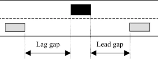
Even if a lane change is desirable or perhaps also necessary it might not be possible or safe to conduct it. In order to evaluate if a driver safely can change lane some kind of gap-acceptance model is generally used. A driver has to decide whether the gap between two subsequent vehicles in the target lane is large enough to perform a safe lane change. This decision-making is generally modeled as evaluating the available lead and lag gaps, see Figure 2.9.
Figure 2.9 Illustration of lead and lag gaps in lane-changing situations.
The common approach is to define a critical gap that determines which gaps that drivers accept and which they don’t. In reality this critical gap varies both among drivers and over time. It also varies between lane changes to the right and to the left and between lead and lag gaps. However, critical gaps are hard to observe, in principle only accepted gaps and to some extent rejected gaps can be measured. Thus, it is hard to measure how critical gaps, for example, vary among drivers and over time for a specific driver. One approach is therefore to use one critical gap for all drivers, but different critical values for lead and lag gaps and for changes to the right and left. This approach is for instance used in the model presented in Kosonen (1999). Even though critical gaps are hard to observe some models has used the approach of using critical gap distributions. For instance, in Ahmed (1999) and later in Toledo et al. (2005) critical gaps are assumed to follow log-normal distributions.
The models in Gipps (1986) and Hidas (2002) are based on a similar but to some extent different approach. Instead of looking at the available and critical gap, a critical deceleration rate is used. In Gipps (1986) a car-following model, namely the model in Gipps (1981), were used to calculate the deceleration rate needed to change lane into the available gap. This deceleration rate was compared to an acceptable deceleration rate. If the deceleration rate needed was unacceptable by the driver, the lane change is not feasible. For lead gaps the car-following model was applied on the subject vehicle with the preceding vehicle in the target lane as leader. For lag gaps the car-following model was applied on the lag vehicle in the target lane with the subject vehicle as the leader vehicle.
The gap-acceptance model also has an important role in the modeling of the urgency of changing lane. When getting closer to an obstacle or an intended turn, i.e. being in zone 2 or 3 in Figure 2.7, drivers are more urgent to get to the target lane. Drivers in these situations generally accept smaller gaps or, following the approach in Gipps (1986) and in Hidas (2002), higher deceleration rates. In Yang and Koutsopoulos (1996) this is modeled by letting the critical gap linearly decrease from a standard critical value to a minimum value with the distance to the critical point for the lane change. The model in Gipps (1986) uses a similar approach where the acceptable deceleration rate increases linearly with the distance left to the intended turn.
2.3.3 Overtaking models
On roads without barriers between oncoming traffic it is not enough to only consider the actual lane change to the oncoming lane. Instead a model that considers the whole overtaking process is needed. As lane-changing decisions, overtaking decisions can be divided into several sub-models or questions. An
Lead gap Lag gap
overtaking decision can for instance be the answer of the following questions, (Brodin et al., 1986):
• Is the overtaking distance free from overtaking restrictions? • Is the available gap long enough?
• Is the driver-vehicle unit able to perform the overtaking? • Is the driver willing to start an overtaking at the available gap?
Drivers generally do not start an overtaking on places with overtaking restrictions. However, not all drivers behave legally in this matter and depending on the proportion of lawbreakers the model may have to account for vehicles that do not obey the present overtaking restrictions. Drivers generally do not start an overtaking if the available gap at the time of the overtaking decision is shorter than the estimated overtaking distance. Another limitation for performing an overtaking can be the overtaking vehicle’s performance, for example maximum acceleration or speed. Even though a vehicle might be able to perform an overtaking, the driver will probably not execute it if the overtaking distance will be unreasonable long, for example more than one kilometer. Even if the driver is able to perform the overtaking it is not sure that he or she is willing to execute it at the available overtaking gap. Drivers’ willingness to accept an overtaking opportunity varies quite a lot. One driver may reject a gap whether another accepts the same gap, and one driver that accepts a gap at one point in time can reject an equal gap at another time.
The drivers’ willingness to accept an available gap is generally modeled with some kind of gap-acceptance model. As in the lane-changing case the most simple way to model this is to use one common critical gap for all drivers, for example as in the model presented in Ahmad and Papelis (2000). However, drivers’ willingness to accept an available gap varies both among drivers and over time for a specific driver. Overtaking models therefore often need more advanced gap-acceptance models compared with the lane-changing case. These models are commonly based on an assumption of either consistent or inconsistent driver behavior. In an inconsistent model, drivers’ overtaking decisions do not depend on their previously overtaking decisions, i.e. every overtaking decision is made independently. The opposite is a consistent driver model, which instead assumes that all variability in gap-acceptance lies between drivers. That is, each driver is assumed to have a critical gap, such that the driver would accept every gap that is longer and reject gaps that is shorter than the driver’s critical gap at all times. According to McLean (1989) there are at least two studies that states that the variance over time for a specific driver is larger than the among driver variance with respect to overtaking decisions. In the first study (Bottom et al., 1978) it was found that more than 85 % of the total variance in gap-acceptance is over time variation for a specific driver, which lead to the conclusion that an inconsistent model would be a more preferable representation of real overtaking gap-acceptance behavior than a consistent model, (McLean, 1989). The high over time variance is however questioned in McLean (1989), which means that the result could have been affected by the experimental design. On the other hand, the second study (Daganzo, 1981) also found that the over time driver variance is larger than the among driver variance. By using statistical estimation techniques this study found that about 65 % of the total variance is over time driver variance, which also supports the use of an inconsistent model. The best way to model
gap-acceptance is of course to use a model that includes both over time and among driver variance. However, a big problem, pointed out in Daganzo (1981), is that it’s very difficult to estimate appropriate distributions for such an approach, (McLean, 1989).
The gap-acceptance behavior does not only vary among drivers and over time, it also varies depending on, for example, type of overtaking and the speed of the overtaken vehicle. McLean (1989) includes a presentation of the following five basic descriptors, also used in the work in Brodin and Carlsson (1986), for classifying an overtaking decision:
• Type of overtaken vehicle: A driver behave differently depending on the type of vehicle to overtake, a driver can for example be expected to be more willing to overtake a truck than a car.
• Speed of overtaken vehicle: The speed affects both the required overtaking distance and the probability of accepting an available gap. • Type of overtaking vehicle: Overtaking behavior can be expected to
differ between for example high performance cars and low-performance trucks.
• Type of overtaking: If a vehicle has the possibility to perform a flying overtake, i.e. start to overtake when it catches up with a preceding vehicle, a driver behave differently compared to situations where the driver first has to accelerate in order to perform the overtaking.
• Type of gap limitation: Drivers’ willingness to start an overtaking also varies depending on if an oncoming vehicle or a natural sight obstruction limits the available gap. Drivers are for instance generally more willing to accept a gap limited by a natural sight obstruction than equal gaps limited by oncoming vehicles.
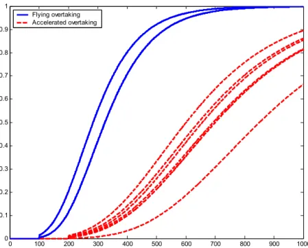
Using these descriptors, the probability of accepting a certain overtaking gap does not only depend on the size of the gap but also on the other descriptors. This leads to a probability function for every combination of descriptors. A quite large data material is needed to estimate all these functions. A couple of studies and estimations of the overtaking probability has been performed, see McLean (1989) for an overview. Figure 2.10 shows examples of probability functions for overtaking situations with an oncoming vehicle in sight. The functions are estimations for Swedish roads presented in Carlsson (1993).
0 100 200 300 400 500 600 700 800 900 1000 0 0.1 0.2 0.3 0.4 0.5 0.6 0.7 0.8 0.9 1
Distance to oncoming vehicle, [m] Flying overtaking
Accelerated overtaking
Figure 2.10 Probability functions for overtaking decisions, combinations of
descriptors with oncoming vehicle in sight, (Carlsson, 1993).
As can be seen in the figure, the overtaking probability for a flying overtaking was estimated to be higher than the probability for an accelerated overtaking at the same available gap.
2.3.4 Speed adaptation models
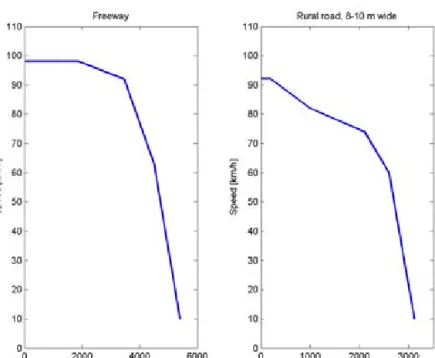
Most micro simulation models use some desired speed parameter to describe drivers preferred driving speed. Generally, a normal distribution is used to model the variation in desired speed among drivers. However, a driver’s desired speed is not constant. The desired speed varies depending on the current road design. On urban roads or freeways, drivers’ desired speed mainly depends on the posted speed limit. However, on rural roads, like two-lane highways the desired speed also varies with for example road width and curvature. In order to model that drivers’ desired speed varies depending on the road design some kind of speed adaptation model is needed.
One possible modeling approach for roads where the speed limit is the only or the main determining factor of the desired speed is to assign each driver a desired speed for each possible speed limit. This gives a flexible model in which it is possible to catch variation in desired speed for different speed limits. A similar but little less flexible way, is to define a relative desired speed distribution. A driver’s desired speed is then calculated by adding the assigned relative speed to the posted speed limit. This approach was for example used in Yang (1997) and Ahmed (1999). In Barceló and Casas (2002) a similar variant is used, in which driver’s desired speeds are deduced by multiplying the posted speed limit with an
individual speed acceptance parameter. The speed acceptance parameter follows a normal distribution among drivers.
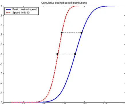
On rural roads, drivers’ desired speed is also affected by the road geometry. The desired speed can for instance depend on the road width or the curvature. Brodin and Carlsson (1986) include a presentation of a speed adaptation model in which a drivers desired speed is affected by the speed limit, the road width, and the horizontal curvature. In this model each driver is assigned a basic desired speed, which is adjusted to a desired speed for each road section. This is done by reducing the median speed according to three sub-models, one for each of the above-mentioned factors. However, a driver’s desired speed is in the model not only the result of a shift of the distribution curve, as in the models presented in Yang (1997), Ahmed (1999), and Barceló and Casas (2002). The desired speed distribution curve is also rotated around its median. This makes it possible to tune the model in such a way that drivers with high desired speeds are more affected by a speed limit than drivers with low desired speeds, see the example in Figure 2.11. 40 60 80 100 120 140 160 0 0.1 0.2 0.3 0.4 0.5 0.6 0.7 0.8 0.9
1 Cumulative desired speed distributions
Desired speed, [km/h] Basic desired speed
Speed limit 90
Figure 2.11 Example of shift and rotation of a desired speed distribution.
How much the curve is rotated depends on which factors that addressed the reduction. Different rotation parameters are used for adaptation caused by the road width, the speed limit, and the horizontal curvature.