DISSERTATION
ANALYSIS OF STRUCTURED DATA AND BIG DATA WITH APPLICATION TO NEUROSCIENCE
Submitted by Ela Sienkiewicz Department of Statistics
In partial fulfillment of the requirements For the Degree of Doctor of Philosophy
Colorado State University Fort Collins, Colorado
Summer 2015
Doctoral Committee:
Advisor: Haonan Wang Mary Meyer
F. Jay Breidt Stephen Hayne
Copyright by Ela Sienkiewicz 2015 All Rights Reserved
ABSTRACT
ANALYSIS OF STRUCTURED DATA AND BIG DATA WITH APPLICATION TO NEUROSCIENCE
Neuroscience research leads to a remarkable set of statistical challenges, many of them due to the complexity of the brain, its intricate structure and dynamical, non-linear, often non-stationary behavior. The challenge of modeling brain functions is magnified by the quantity and inhomo-geneity of data produced by scientific studies. Here we show how to take advantage of advances in distributed and parallel computing to mitigate memory and processor constraints and develop models of neural components and neural dynamics.
First we consider the problem of function estimation and selection in time-series functional dynamical models. Our motivating application is on the point-process spiking activities recorded from the brain, which poses major computational challenges for modeling even moderately com-plex brain functionality. We present a big data approach to the identification of sparse nonlinear dynamical systems using generalized Volterra kernels and their approximation using B-spline basis functions. The performance of the proposed method is demonstrated in experimental studies.
We also consider a set of unlabeled tree objects with topological and geometric properties. For each data object, two curve representations are developed to characterize its topological and geometric aspects. We further define the notions of topological and geometric medians as well as quantiles based on both representations. In addition, we take a novel approach to define the Pareto medians and quantiles through a multi-objective optimization problem. In particular, we study two different objective functions which measure the topological variation and geometric variation respectively. Analytical solutions are provided for topological and geometric medians and
quantiles, and in general, for Pareto medians and quantiles the genetic algorithm is implemented. The proposed methods are applied to analyze a data set of pyramidal neurons.
ACKNOWLEDGEMENTS
First and foremost I would like to express my deepest appreciation and gratitude to my advisor Professor Haonan Wang for his invaluable mentorship and inspiration throughout our research collaboration. I am especially grateful for his limitless patience and advice in the process of writing this dissertation.
I would also like to thank my committee members Professors Mary Meyer and Jay Breidt for the important and insightful feedback they provided to me for my dissertation work, and for their guidance and advice during my years at Colorado State University.
Next, I would like to thank my outside committee member Dr. Stephen Hayne from the De-partment of Computer Information Systems and Dr. Christos Papadopoulos from the DeDe-partment of Computer Science for providing me with access to their computer labs, without which parts of this dissertation could not have been written. In addition, I would like to thank Dr. Hayne for the valuable comments and suggestions he provided on this dissertation.
I would also like to thank Dr. Dong Song from the Center for Neural Engineering at the Uni-versity of Southern California for his indispensable contributions to Chapter 2 of this dissertation, as well as his professional advice and valuable comments.
I would also like to express my gratitude to the Department of Statistics at Colorado State University for all of their support and for creating a friendly, stimulating environment.
Lastly, I would like to thank all of my family and friends for supporting me through these challenging five years.
TABLE OF CONTENTS
ABSTRACT . . . ii
ACKNOWLEDGEMENTS . . . iv
LIST OF TABLES . . . viii
LIST OF FIGURES . . . xiv
Chapter 1 - Introduction . . . 1
1.1 Background . . . 1
1.2 Scope . . . 4
Chapter 2 - Sparse Functional Dynamical Models . . . 7
2.1 Introduction . . . 7
2.2 Map-reduce and Big Data . . . 11
2.2.1 Computational Complexity Analysis . . . 11
2.2.2 A Brief Review of Map-Reduce . . . 13
2.2.3 Matrix processing . . . 14
2.3 Multiple-Input and Single-Output Model . . . 17
2.3.1 Volterra Model . . . 17
2.3.2 Kernel Functions and Basis Functions . . . 19
2.3.3 Likelihood and Parameter Estimation . . . 21
2.3.4 Functional Sparsity and Neural Connectivity . . . 22
2.4.2 Maximum Likelihood Estimation with Conjugate Gradient . . . 25
2.4.3 Penalized Maximum Likelihood Estimation . . . 27
2.4.4 L1 Regularization via Coordinate Descent Algorithm . . . 29
2.4.5 Tuning Parameters . . . 29
2.5 Data Analysis . . . 30
2.5.1 Analysis of Neural Spikes . . . 30
2.5.2 First-Order Model . . . 31
2.5.3 Second-Order Model . . . 35
2.5.4 Model Validation . . . 39
Chapter 3 - Pareto Quantiles of Unlabeled Tree Objects . . . 41
3.1 Introduction . . . 41
3.2 Data Object and its Curve Representation . . . 45
3.2.1 Data . . . 45
3.2.2 Graph as a Data Object . . . 46
3.2.3 Curve Representations for Unlabeled Trees and Forests . . . 49
3.2.4 Equivalence Classes of Topology and Geometry . . . 51
3.3 Methodology . . . 53
3.3.1 Median Trees and L1 Distance . . . 53
3.3.2 Pareto Median Trees — A Multi-Objective Approach . . . 56
3.3.3 Pareto Quantiles of Unlabeled Trees . . . 60
3.3.4 Genetic Algorithm . . . 61
3.4 Real Data Analysis . . . 63
3.5 Simulation Study . . . 71
3.5.2 Neuron topology . . . 73 3.5.3 Tree Reconstruction . . . 77 3.5.4 Simulation Results . . . 78 3.6 Proofs . . . 81 3.6.1 Proof of Theorem 1 . . . 81 3.6.2 Proof of Theorem 2 . . . 82 3.6.3 Proof of Theorem 3 . . . 84 3.6.4 Proof of Theorem 4 . . . 85 3.6.5 Proof of Theorem 5 . . . 86
Chapter 4 - Genetic Algorithm for Tree-Structured Data . . . 88
4.1 Introduction . . . 88
4.2 Genetic Algorithm for Tree Objects . . . 89
4.3 Encoding . . . 89
4.4 Selection . . . 90
4.5 Reproduction and Feasibility . . . 91
4.6 Replacement . . . 94
4.7 The best topology for a geometry . . . 94
Chapter 5 - Future Work . . . 95
LIST OF TABLES
2.1 Performance results for the second-order model with map-reduce for different hardware configurations. . . 35
3.1 Comparison of Cmand Tmfor m = 1, . . . , 10. Here, Cmrepresents the Catalan number,
LIST OF FIGURES
2.1 Map-Reduce architecture with mappers and reducers running on one or multiple servers. 14 2.2 Mapper and reducer functionality for XTy. . . 15 2.3 Mapper and reducer functionality for XTX. . . 15 2.4 Mapper and reducer functionality for XTXβ. . . 16 2.5 Second-order Volterra model with d inputs and one output. Inputs are convoluted
with ϕ functionals of first- and second-order. The history of output y is treated as an additional input. . . 20 2.6 Top: A sequence of 13 cubic B-spline basis functions with 9 equally-spaced interior
knots on the interval [0,1]. Bottom: An illustration of a function with local sparsity on interval [0,0.2]. There are 10 subintervals corresponding to 10 groups. On each subinterval, there are 4 basis functions coefficients taking positive values. For instance, to identify the sparsity of the function on [0, 0.1], all four basis functions (dashed line type) need to have coefficients zero. . . 23 2.7 Three-second recording (out of 90 minutes) of seven inputs x1, . . . , x7 (top rows) and
output y (bottom row). . . 31 2.8 Maximum likelihood estimation (solid) and penalized maximum likelihood
estima-tion using a group bridge penalty (dashed), SCAD (dotted) and LASSO (dash-dotted) of ϕ functionals in the first-order model corresponding to the input neurons: x1, x2, x4, x6. The estimates are comparable, and only a zoom-in view highlights
2.9 Maximum likelihood estimation (solid) and penalized maximum likelihood estimation using a group bridge penalty (dashed), SCAD (dotted) and LASSO (dash-dotted) of ϕ functionals in the first-order model corresponding to the input neurons: x3, x5, x7.
No sparsity is detected. . . 33 2.10 Maximum likelihood estimation (solid) and a group bridge estimation (dashed) of a
ϕ functional in the first-order model corresponding to the output neuron. Local sparsity is not detected. . . 34 2.11 Maximum likelihood estimation (solid) and a group bridge estimation (dashed) of ϕ
functionals in the second-order model corresponding to the input neurons x1, x3,
x4, x5, x6, x7. Local sparsity visible for the penalized version in all neurons, the
start of sparsity is marked with an arrow. Neuron x2 exhibits global sparsity. . . . 37
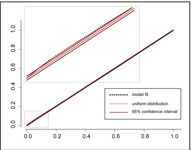
2.12 Penalized estimation of interaction components in the second-order model. Only non-zero components are displayed. . . 38 2.13 KS plot for rescaled firing probabilities against a reference distribution (uniform).
Rescaled firing probabilities are depicted with a thick dashed line, reference uniform distribution with a dotted line, and a 95% confidence interval with a thin solid line. Small bias is visible for low probabilities, more evident in the zoom-in subplot. . . 40
3.1 Graphical display of a pyramidal neuron cell, named after its pyramid-like shape. . . . 42 3.2 Graphical display of six neurons. Top row: three neurons from CA1 region of
hip-pocampus; Bottom row: three neurons from CA3 region of hippocampus. In each subplot, apical dendrites are shown in magenta and basal dendrites are shown in green. . . 46 3.3 (A) Graphical illustration of a synthetic tree; (B) Dyadic representation using thickness
correspondence; (C) Dyadic representation using descendant correspondence; (D) Harris path for the tree in (B); (E) Harris path for the tree in (C). . . 48
3.4 An example of tree (left) and its curve representations (right): the topological curve (B), the geometric curve (C). . . 51 3.5 A graphical display of a joint geometric tree curve (middle) and topological (bottom)
for the corresponding neuron object (top) with apical dendrites (colored in ma-genta) and basal dendrites (colored in green). . . 52 3.6 A graphical display of the topological median (lower-left panel) and geometric median
(lower-right panel) of a sample of three tree-structured objects (top row). The number associated with each branch segment is the segment length, and is referred to as a geometric attribute. Here both median trees have the same topological structure with three branch segments. . . 55 3.7 A graphical display of the topological median and geometric median of a sample of
three tree-structured objects. Topological Median is the same as shown in Figure 3.6. . . 56 3.8 (A) Graphical display of a sample of 21 simulated trees with the same topology and
different geometric attributes; (B) Topological median tree; (C) Geometric median tree. . . 57 3.9 A graphical display of the Tn-values (horizontal axis) and Gn-values (vertical axis) for
all Pareto median trees. The solutions form a Pareto front. In particular, the tree objects corresponding to those values are shown in panels (A)-(D). . . 59 3.10 Top row: Pareto set for the 25th quantile; bottom row: Pareto set for the 75th quantile.
Trees A and C are geometric Pareto quantiles, and trees B and D are topological Pareto quantiles. . . 62
3.11 A graphical display of the Pareto set for the median of apical dendritic trees from CA1. The solutions form a Pareto front. The geometric Pareto median (A) and topological Pareto median (D) as well as two other Pareto medians, (B) and (C), are highlighted. All four are depicted in Figure 3.14. Here both axes are shown in log-scale. . . 63 3.12 (A) Joint geometric curves for all neurons from CA1 region; (B) Joint topological
curves for all neurons from CA1 region; (C) Joint geometric curves for all neurons from CA3 region; (D) Joint topological curves for all neurons from CA3 region. . . 65 3.13 Graphical display of topological and geometric tree curves, as well as corresponding
tree objects, for geometric Pareto median (top row) and topological Pareto median (bottom row) . . . 66 3.14 Pareto median trees from CA1, including the geometric Pareto median (panel A), the
topological Pareto median (panel D), and two other Pareto median trees (panels B and C). The Tn and Gn values for those four median trees are highlighted in
Figure 3.11. . . 67 3.15 Topology for the median apical dendrite from CA1: pointwise true value (solid line)
and two labeled methods (dotted and dashed lines). Overall numbers of branches are shown in brackets. Labeled methods underestimate the number of dendritic segments. . . 68 3.16 Graphical display of topological and geometric tree curves, as well as corresponding
tree objects, for geometric 10th Pareto quantile (top row) and topological 10th Pareto quantile (bottom row). . . 69 3.17 Graphical display of topological and geometric tree curves, as well as corresponding
tree objects, for geometric 90th Pareto quantile (top row) and topological 90th Pareto quantile (bottom row). . . 70
3.18 Left: Estimated mean rate functions for length of branches in two types of dendrites from CA1 using Negative-binomial model. Right: Estimated probability function of the branch bifurcation for two types of dendrites from CA1. (Solid line: apical dendrites; Dashed line: basal dendrites). . . 74 3.19 An example of incompatible geometric (A) and topological (C) curves with the same
number of internal nodes m = 3. Tree in panel (B) has the geometric tree curve (A), and tree in panel (D) has the topological tree curve (C). . . 76 3.20 A sample of simulated neuron objects. The angles between branches are chosen for
improved visibility. . . 78 3.21 Topological (left) and geometric (right) pareto population median (black) and
sam-ple 95% confidence intervals (grey). The population medians are within the 95% confidence interval. . . 79 3.22 (A) 10th, (B) 25th, (C) 75th and (D) 90th topological Pareto population quantiles
(black) and sample 95% confidence intervals (grey). The population quantile is within the 95% confidence interval. . . 79 3.23 (A) 10th, (B) 25th, (C) 75th and (D) 90th geometric Pareto population quantiles
(black) and sample 95% confidence intervals (grey). The population quantile is within the 95% confidence interval. . . 80
4.1 Chromosome-like encoding for trees in the toy example from Figure 3.7. . . 90 4.2 An example of a compressed chromosome for an apical tree. There are 40 genes in this
4.3 Three types of mutations. The center element in the left-most box (marked in grey) is selected for a mutation. The numbers above the arrow are randomly selected, in the range determined by the symbol count. Panel (A): a mutation modifies a branch by moving a node; panel (B): a mutation adds a branch; panel (C): a mutation deletes a branch. Mutations in panels (A) and (B) have two subtypes and each is selected with an equal probability. The probabilities of applying (A), (B) or (C) can be equal or configurable. . . 93
CHAPTER 1
Introduction
1.1 Background
Statistical analysis has been an integral part of neuroscience ever since the discovery of the stochastic nature of neural responses. Scientists were using electrodes to detect neural action potentials, also referred to as neural spikes, in the brains of animals as early as the 1950s. At the time, the dominating theories of neural activity were deterministic, but experiments showed variability in the response when the stimulus was held constant, and random spikes in the absence of any stimuli. See Stein [1965] for a theoretical analysis of that variability, and Harrison et al. [2013] for a recent review of statistical modeling of variability and its counterpart synchrony, detected in various parts of the nervous system.
Neuroscience research generates a great deal of public interest, from the dynamics of learning and memory formation to the recognition and diagnosis of brain diseases like autism, depression and Alzheimer’s disease. These and many other goals were behind the recent BRAIN initia-tive (Brain Research through Advancing Innovainitia-tive Neurotechnologies), a governmental program funding and encouraging interdisciplinary effort to provide measurable progress in brain science. Statistics plays an important part in that effort, which was clearly and eloquently discussed in an ASA white paper [ASA, 2014]. The primary statistical tasks will naturally include building models and quantifying uncertainty. Challenges are numerous, especially with regard to account-ing for complex, structured data, spatio-temporal effects, missaccount-ing or incomplete data, variations between species, genders, brain regions, etc. Because of the sheer quantity of data produced by neuroscience research, the analysis often enters the realm of big data, where many classical methods become impractical due to memory or time constraints; see Fan et al. [2014] for a recent
The brain is a source of big data due to its massive structure comprised of billions of neural cells and trillions of connections, but in reality, the brain’s structure is not static. In fact, it is continuously evolving with changes driven by complex dynamic behavior. The behavior and the structure, two important aspects of the brain, are interconnected with one impacting the other. So far we are lacking sufficient quantities of data that would combine these characteristics, but the potential for future research is enormous.
The dynamic aspects of the brain include the exchange of electric signals (action potentials) between neural cells. Neurons typically consist of a soma, an axon and one or more types of dendrites; see Figure 3.1 for an example of a neuron and its components. Dendritic structures of neurons are responsible for receiving signals from other cells, whereas an axon carries the signal outside of the cell. The history of a single neuron’s firings is often encoded as a spike train. Analysis of neural spike trains is at the core of much contemporary neuroscience research. Researchers model output neural spikes based on the inputs to understand the behavior of neurons in various regions of the brain, e.g., a frequently modeled brain region is the hippocampus, an area involved in learning and memory formation. The dependency between inputs and outputs is non-linear, temporal, and often non-stationary. In fact, the spatio-temporal patterns of neural firings are believed to be a part of information encoding in the brain.
There are many approaches to the analysis of spike trains, each with numerous examples in the literature, e.g., Bayesian analysis [Archer et al., 2013], firing intensity estimation with a Cox proportional hazard model [Brown et al., 2002, Plesser and Gerstner, 2000], Artificial Neural Networks based model [Maass, 1997], and a logistic model with generalized Volterra kernels [Song et al., 2007, 2013]. Each model has been useful in answering important research questions, but each also comes with challenges and shortcomings. One of the major challenges is dimensionality. Usually, output neural spikes depend not just on current but also past input observations, and system memory is large relative to the duration of a spike. These assumptions, together with
complex interactions between inputs, can lead to the estimation of thousands of parameters even for a system with a relatively small number of inputs. One of the contributions of this dissertation is presenting a strategy for fitting sparse dynamical models to neural data using appropriate optimization methods, approximations, and parallel computing.
The brain can be viewed as a complex network with a small world architecture. The connec-tions between cells are not observed directly, but can be modeled based on the analysis of spike train firings. A cell’s propensity to form these connections has also been of interest to scientists. The more complex the dendritic structure, the more signals a cell can potentially receive and pro-cess [Mel, 1999]. As early as the nineteenth century, scientists observed a correlation between the diversity of neural dendritic structures and the complexity of the entire organism; see Ram´on y Cajal [1995] for a detailed study of the nervous systems of vertebrates. The heterogeneity of dendritic structures has also been associated with learning capabilities. Some early methods to estimate the density of dendritic arborizations included the counting of dendritic segments and the calculation of a fractal dimension [Fiala and Harris, 1999]. Dendritic structures can be mod-eled as trees, often as binary trees. Trees are complex, extremely non-Euclidean structures, and classical statistical tools are often not sufficient to describe and quantify them. Due to the het-erogeneity encountered in the real biological tree-structured data, it is often desirable to compare not just the mean structures of samples, but also objects representing different quantiles, e.g., 10th or 90th, of the corresponding distributions. For such comparisons to be possible, a notion of a quantile of tree-structured data is required. A space of complex data lacks a natural order, just like multivariate and functional data. In the analysis of multivariate and functional data, the simplicial depth [Liu, 1990] and norm minimization [Serfling, 2002, Walter, 2011] have been applied to define analogs of the order statistic. The analysis of tree objects has been, until the last decade, focused on classification trees [Banks and Constantine, 1998, Phillips and Warnow,
and a median tree are of particular interest, and popular approaches were built on the notion of the Fr´echet median [Fr´echet, 1948]. Only recently, with advances in medical imaging technologies, biological tree-structured data have become available to statistical analysis. In a study motivated by the analysis of the structure of brain arteries, Wang and Marron [2007] provided the first attempt to define a median of a set of trees with both topological and geometric properties. The approaches in that and many other papers [Aydın et al., 2009, Wang et al., 2012] were based on labeling of tree nodes for correspondence between branches. Such nodal correspondence may be natural in some applications. For instance, nodes in classification trees and edges in phylogenetic trees are uniquely identified. This is not always the case in biological data, as with plant roots, brain arteries and dendritic arborizations. Various choices of correspondence can potentially lead to different research conclusions, and artificially imposed labeling may result in biased estimates. For example, Skwerer et al. [2014] observed that labeling in trees serving as a model of human brain arteries can lead to a degenerate, star-tree median. For trees where labeling is not natural, it can be beneficial to consider quantiles that do not depend on assigned labels. The analysis of unlabeled tree-structured data has not been addressed before now and is a major contribution of this dissertation.
1.2 Scope
In this dissertation, we develop statistical models motivated by two data sets originating from neuroscience research, specifically, a large set of dynamic data consisting of spike trains recorded in animal studies, and a set of complex, structured objects extracted from digital reconstructions of neurons. Both data sets pose a big data challenge.
In Chapter 2, we propose a numerical implementation of sparse functional dynamical models with a large data set. Our motivating example comes in the form of spike train data collected from the hippocampus of a rodent. The data consists of 90-minute recordings of activities from eight
hippocampal neural clusters, and our goal is to develop a Multiple-Input Single-Output (MISO) system, which models an output neuron as a function of its current and past inputs. Our work builds on ideas proposed by Song et al. [2007, 2013], and it employs a probit model with a Volterra series. A Volterra series is a generic solution to nonlinear differential equations, and, similar to a Taylor series expansion, approximates a function with a desired accuracy on a compact set. Unfortunately, for most large data sets, only the first order model is computationally feasible, even if the model fit is not considered adequate. This is in part due to the massively large number of parameters in the model. Our contribution is a feasible and efficient computational strategy to fit second- and higher-order Volterra models using the maximum likelihood principle and its regularized analog. Our proposed strategy uses a smaller memory footprint and makes model fit feasible on a multi-core computer without paying a penalty for distributed computations.
In Chapter 3, we focus our attention on complex, non-Euclidean data, specifically tree-structured data, that can be characterized as highly heterogeneous. Most work in the literature focuses on the topological properties of trees based on pre-selected labeling systems. Here, we take both topological and geometric attributes of trees into account, and intend to develop statistical tools for unlabeled trees. Our goal is to define quantiles of such objects, which can be potentially used for comparison between samples of tree-structured data. In particular, we develop a con-cept of a quantile of tree-structured objects through a multi-objective optimization problem. We include criteria that quantify topological and geometric variations as objective functions in the optimization problem. We also develop a methodology to identify empirical quantiles for a sample of tree-structured data. Identification of empirical quantiles is a high-dimensional, combinatorial optimization problem. Such a problem can often be solved efficiently with a genetic algorithm, which has been shown to exhibit an implicit parallelism; see Goldberg [1989]. In Chapter 4, we discuss in details the genetic algorithm used in estimating empirical quantiles of unlabeled tree
Finally, in Chapter 5, we discuss future work in the direction of one-sample and two-sample hypothesis testing of unlabeled tree-structured data, based on mixtures of topological tree distri-butions and simulations.
CHAPTER 2
Sparse Functional Dynamical Models
12.1 Introduction
Dynamical system is time-dependent, i.e., its output is determined not only by its current input, but also its past inputs. Its complexity is often enhanced by the nonlinear interactions within its internal structure, in such a way that the resulting system is different from the sum of their parts. It has been shown that despite their complex nature, dynamical systems can often be described with a few low order ordinary differential equations; see Fuchs [2013] for a more recent review.
The first documented study of a nonlinear dynamical system involved two interacting species, predators and prey, and was conducted independently by Volterra and Lotka in the 1910s and 1920s. The interaction was modeled through nonlinear differential equations [Volterra, 1930]. The Volterra series has been demonstrated to be a general solution to such nonlinear differential equation [Flake, 1963, Karmakar, 1979, Volterra, 1930]. It represents the output of the system as a series of convolutions of its inputs and is often referred to as a Taylor series with memory, or a nonparametric representation of a nonlinear system. For a system with a single input x(t) and a single output y(t), the series can be expressed in the following form
y(t) = κ0+ ∞ X p=1 Z ∞ −∞ · · · Z ∞ −∞ κp(τ1, . . . , τp)x(t − τ1) · · · x(t − τp)dτ1· · · dτp (2.1)
where κp is known as the p-th order Volterra kernel. In practice, all Volterra kernels have to be
estimated in the process of system identification.
The Volterra theory of analytic functions was advanced by Wiener in the applications to elec-tronic communications in the 1920s [Wiener, 1958], which resulted in a Wiener theory of nonlinear
systems. The key idea of the Wiener series was to orthogonalize the Volterra functionals, and thus facilitate model estimation. By the 1950s both the Volterra and Wiener models became accepted and widely-used methods of the analysis of complex dynamical systems with finite memory and time-invariance. Just like the Taylor series for nonlinear functions, the Volterra/Wiener series can suffer from convergence issues, but in 1910, Fr´echet showed that the Weierstrass theorem can be extended to Volterra functions, essentially proving that any Volterra/Wiener system can be approximated on a compact set with a desired accuracy [Fr´echet et al., 1936].
The nonlinear dynamical systems have been identified in areas as diverse as social science, natural science and engineering. In economics and psychology the system dynamics are related to human behavior and interactions. Engineering processes, although usually described by a set of known rules or laws, can exhibit unknown nonlinearities, especially under abnormal circum-stances, e.g., in control systems. The systems analyzed by Wiener and Schetzen [Schetzen, 1981, Wiener, 1958] considered inputs like voltage, current, velocity, stress, temperature. A network monitoring system is concerned with traffic characteristics: volume, temporal and spatial pat-terns of messages, etc. Nonlinear interactions between inputs are modeled to describe and detect system failures, network intrusions, resource misuse, etc [Cannady, 1998, Debar et al., 1992].
Biological systems present a much greater challenge, since the rules governing their behavior are unknown or only partially understood. They are frequently modeled as black-boxes or gray-boxes with multiple inputs and multiple outputs. There are abundant examples of applying the Volterra or Wiener functional expansion in modeling physiological functions: cardiovascular, respiratory, renal [Marmarelis, 1993], functions of auditory peripherals and visual cortex [Wray and Green, 1994], human pupillary control, medical imaging [Korenberg and Hunter, 1996] and many more.
The particularly challenging examples of biological systems come from neuroscience, with the human brain considered to be the most complex nonlinear dynamical system of all. It is also a
good illustration of a system composed of subcomponents, in which understanding the function-ality of simplest building blocks is not enough to understand and model the entire system. The behavior of neurons, each one consisting of a soma, an axon, and dendrites, has been fairly well understood at the individual level. Existing parametric models (e.g., Hodgkin-Huxley, Fitzhugh-Nugamo, Hindmarsh-Rose), consisting of sets of differential equations, can successfully describe the nonlinear dynamics of the membrane voltage at single neuron level [Fuchs, 2013]. However, these models cannot easily scale up to the level of neural ensembles, which are groups of intercon-nected and functionally similar neurons, due to numerous unknown biological mechanisms and processes within the neuronal networks. On the other hand, nonlinear dynamical model in the form of the Volterra/Wiener series, models the neural ensembles directly from their input/output data. It does not rely on the complete knowledge of the system and thus provides an appealing approach for modeling large-scale, complex nervous systems.
Specifically in this paper, we model the nonlinear dynamics of neural ensembles using spiking activities. Spikes, also termed action potentials, are brief electrical pulses generated in the soma and propagating along axons. Neurons receive spike inputs from other neurons through synapses and then transform these inputs into their spike outputs. This input-output transformation is determined by numerous mechanism/processes such as short-term synaptic plasticity, dendritic/-somatic integration, neuron morphology, and voltage-dependent ionic channels. Since spikes have stereotypical shapes, they can be simplified as point-process signals carrying information with the timings of the pulses. It is widely accepted that, in the brain, information is encoded in the spatio-temporal patterns of spikes. Thus, characterization of the point-process input-output properties of neurons using spiking activities is a crucial step for understanding how the neurons, as well as the neuronal networks, transmit and process information; see Song et al. [2007, 2013]. Within a neural ensemble, this procedure is essentially the identification of the functional connectivity
In the previous studies (Song et al., 2007, 2009), Volterra kernel models were combined with generalized linear models to characterize the input-output properties of neurons. To facilitate model estimation, Volterra kernels are expanded with basis functions, e.g., Laguerre basis or B-spline basis. Model coefficients are estimated with a penalized likelihood method (Song et al., 2013). However, this model estimation imposes major computational challenge. The first-order Volterra series has been shown to be inadequate to capture the system dynamics [Song et al., 2007]. The second-order series, with even a moderate number of inputs and basis functions, requires an estimation of thousands of parameters. A large number of observations is critical, to account for sparsity in the inputs and to avoid over-smoothing of the basis functions; see Marmarelis [1993] and remarks by Korenberg and Hunter [1996].
With a large n and a large p, the system identification faces a big data challenge, which is characterized by both hardware and software issues; see Fan et al. [2014] for a recent review. The data may not fit in the memory of a single computer, and some statistical methods, if they can be adjusted to accommodate distributed data and computing, just take too long to be computationally feasible. As a result, none of the cited papers was successful in providing a viable and reproducible method of regularized estimation of Volterra kernels of higher orders. A regularization is key to achieve a functional sparsity at both local and global levels, necessitated by the sparsity in neural connectivity [Tu et al., 2012]. Song et al. [2013] provided a nice study of sparsity by comparing the effects of Laguerre basis and B-spline basis. Both types are adequate in representing the global sparsity, but only the B-spline basis successfully model the local sparsity. It is worth mentioning that, to achieve sparsity, Song et al. [2009] used the forward step-wise model selection and Song et al. [2013] implemented regularization based method, e.g., LASSO [Tibshirani, 1996].
Aside from the nonparametric modeling using Volterra kernels, other approaches are also available though they are not considered in this paper:
• Cascade or block structure modeling [Korenberg and Hunter, 1986]
• Basis representation of orthogonalized Wiener kernels [Marmarelis, 1993].
• Artificial neural networks (ANN) [Wray and Green, 1994], the authors show a correspon-dence between the Volterra kernel model and a neural network. Recurrent neural networks are a competing approach to the analysis of the nonlinear dynamical systems, and can perform both a knowledge based, and a black-box type system identification.
In this paper we address the aforementioned computational challenges by applying big data techniques to perform a system identification using a sparse basis expansion of the Volterra kernels of a second or higher order. The rest of this paper is organized as follows. Section 2.2 contains an overview of the map-reduce technique. Section 2.3 presents our proposed dynamical Multiple Input Single Output (MISO) model. Section 2.4 describes the computational issues and Section 3.2 covers the analysis of real data.
2.2 Map-reduce and Big Data
2.2.1 Computational Complexity Analysis
Given the disparity between our perception of time and the small scale of inter-neural com-munication, the analysis of brain functions is bound to face computational challenges. A short 15 minute recording of brain activity in an animal performing stimuli-induced actions can lead to close to a million observations if broken into 1 millisecond (ms) intervals, a timeframe in which a neural spike can be detected. The number of the input connections doesn’t have to be large (in fact the neural network is believed to exhibit a small-world architecture: few direct connections, but only a few steps away from any other neuron [He, 2005]), but due to complex interactions between inputs, even a small number of them can lead to thousands of parameters in the model.
memory requires just close to 2 GB of storage, but for the second-order system that number grows to over 200 GB, and involves close to thirty thousand parameters. Many matrix operations are “embarrassingly parallel”, so an infrastructure is needed to divide the matrix into chunks that can fit in the memory of a single computer, execute tasks in parallel and assemble the results. The division of tasks and reassembly of results are the foundation of the map-reduce approach [Dean and Ghemawat, 2008], an algorithmic concept that can be implemented on a single multi-core system or in a cluster of servers. There exists a variety of multimulti-core programming options, depending on the platform and the language of choice. The most common cluster implementa-tions come from Apache Software Foundation projects, i.e., Hadoop and Spark, and are briefly described in the next section. Although 200 GB may not be considered big data by practitioners dealing with terabytes or more, it is still enough to cause computational issues in the statistical analysis that requires hundreds (and sometimes thousands) of such large matrix operations. Just the generation of a 200 GB matrix took five hours of a single-threaded processing (which could be parallelized). We found two viable computational approaches to the analysis we describe in details in the following sections. The first approach relies on placing the large matrix on the distributed file system, and using the distributed map-reduce framework, e.g., Hadoop or Spark, to perform computations. The cluster should be large enough to offset the penalty of creating and accessing the matrix, and of distributed computing. Without such a large cluster, one can still find a feasible in-memory approach. As will be explained in the following sections, one can fit a higher-order Volterra model with only a first-order model matrix physically existing, and generating higher order data on demand, when performing matrix vector operations. Such ap-proach allowed us to use map-reduce on a single multicore server with very good results, which are detailed in Table 2.1. Gains from such approach can be measured in days of computations relative to a small distributed cluster.
2.2.2 A Brief Review of Map-Reduce
The idea of map-reduce originated at Google [Dean and Ghemawat, 2008] where its original purpose was to accommodate large matrices in data analysis. The matrix and associated computa-tions would be distributed across multiple servers configured into a cluster. Apache Hadoop is an open source implementation of a distributed data storage (DFS) and the map-reduce algorithm. It provides a necessary infrastructure to distribute the data across servers, and an application programming interface (API) for processing chunks of data and assembling the results. The con-cept of map-reduce was adopted in the industry largely due to the availability of the Apache implementation and the option to “lease” a Hadoop cluster from Amazon Web Services. Cur-rently Apache Hadoop is one of the most popular platforms for the statistical analysis of big data, including both supervised and unsupervised learning. A competing map-reduce implementation comes from another Apache project, Spark, and is considered to be a better solution for statistical analysis based on iterative large matrix operations, e.g., Iteratively Re-weighted Least Square or Conjugate Gradient described in Section 2.4.
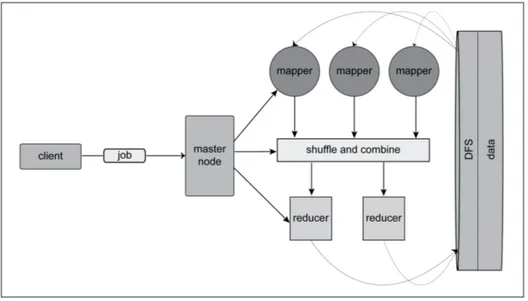
Figure 2.1 depicts the architecture of a generic map-reduce cluster. A client submits a job to the master node, with clearly specified tasks for a mapper and a reducer as well as the location and format of the input data. The master node starts a sufficient number of mappers to execute the job, passing each one a chunk of the input data. The functionality of mappers and reducers is application specific; in fact, the mappers and reducers can perform any tasks, bound only by the format of their input and output. In general, the mapper performs grouping, sorting or filtering functions, and the reducer calculates the summary of the data. Each mapper processes a chunk of data, independent from other mappers, with the results returned in the form of <name,value> pairs, also referred to as keys. A mapper can produce any number of keys as a result, recognizing
vector operations in map-reduce framework are provided in Section 2.2.3. Hadoop mappers and reducers are stateless, and this can become a limitation in an analysis that requires many iterative map-reduce operations. To solve this, Spark allows to execute many mappers and reducers in whichever order, and maintains a context between them. Mappers and reducers can also run within the same process in different threads or on different cores of a multicore server. Many big data applications, including classification and clustering, can benefit from map-reduce based computations, whether in a distributed environment or on a multi-core platform [Chu et al., 2007].
Figure 2.1: Map-Reduce architecture with mappers and reducers running on one or multiple servers.
2.2.3 Matrix processing
In classical statistical analysis, e.g., linear models and generalized linear models, one typically needs to calculate Xβ, XTW y, XTW X, for a design matrix X, a response vector y, a parameter vector β and a weight matrix W . All these operations can be performed using the map-reduce technique with a matrix X stored in a distributed file system. For better illustration, we consider three toy examples as depicted in Figures 2.2-2.4.
Figure 2.2: Mapper and reducer functionality for XTy.
In Figure 2.2, we consider the application of the map-reduce technique to matrix multiplication of a matrix and a column vector, say XTy. Here, X is an n × p matrix with n >> p, and y is a n × 1 vector. In particular, a mapper receives a subset of rows of X, multiplies them by a corresponding subset of elements of a vector y and creates a resulting vector of size p. A reducer adds all output vectors created by the mappers together to produce the desired vector.
Figure 2.3 illustrates another widely used matrix operation in statistics. In order to compute XTX for a matrix X with large n, a mapper receives a subset of rows of X and creates a resulting square matrix of size p × p. A reducer adds all matrices created by mappers. When p is small the resulting p × p matrix is easily invertible in memory.
As indicated by Figures 2.2 and 2.3, the weights can be easily incorporated into the procedures to produce XTW y and XTW X. In fact, when n is large and p is small, the implementation of map-reduce technique is rather straightforward. However, for a large p, it becomes quite complicated. In this paper, within the scope of a large design matrix X of dimension n × p, two detailed categories can be identified
(i) p is moderately large so that p × p square matrix is not easily invertible, but fits in memory;
(ii) p is extremely large, and p × p matrix does not fit in memory.
The category (ii) is more problematic, and may require alternative methods to circumvent matrix inversion; see Section 2.4.2 for further discussion. In the dataset under analysis, the response vector fits in-memory, so the operations XTy and Xβ can be easily performed using the map-reduce technique, but it is the XTW X that can be a source of computational challenges. The size of the parameters vector for the first-order Volterra model belongs to the category (i), but for the second-order and higher, it is in the category (ii). As will become evident in later sections, in many statistical problems the matrix XTW X is only used in a matrix-vector product XTW Xβ, so the large p × p matrix XTW X does not need to be created at all. The matrix-vector product
can be calculated as a single operation in the map-reduce framework. The simplified case with identity weights is visualized in Figure 2.4.
2.3 Multiple-Input and Single-Output Model
2.3.1 Volterra Model
The output of a neuron or neural ensemble consists of a series of spikes, and it is convenient to model it in terms of a probability or a rate of action potentials. Let y(t) be the output signal and let x1(t), . . . , xd(t) (0 ≤ t ≤ T ) be d binary input signals indicating the times at which the spikes
occurred in a T seconds interval. In particular, both input and output signals are recorded at a fixed sampling frequency; that is, for each signal, observations are obtained at t = δ, 2δ, . . . , nδ and T = nδ, where δ is the length of a sampling time interval. At time t, if a spike is observed, then 1 is recorded and 0 otherwise. Although the neural membrane potential is a continuous function, identification of a spike is outside of the scope of this paper, and we will not make any assumptions about the duration of a spike.
Let x(t) = (x1(t), . . . , xd(t))T be the vector of input signals. The conditional probability of
the action potential of the output signal, given the history of the input and output signals, can be written as
θ(t) = P (y(t) = 1|H(t)),
where H(t) = (xT(t), xT(t − δ), . . . , xT(t − mδ), y(t − δ), . . . , y(t − mδ))T. Here M = mδ is the length of the system memory. An intuitive approach is to use the generalized functional additive model with an appropriate link function. There are two common choices: logit and probit link functions. In this paper, we will use the probit link for illustration purpose.
In Song et al. [2007], the authors proposed a discrete generalized Volterra model. The idea is to discretize each kernel function and represent it as a vector of coefficients. For simplicity, we
present their second-order model Φ−1(θ(t)) = κ0+ d X i=1 m X k=0 κ(1)i (k)xi(t − kδ) + d X i1=1 d X i2=1 m X k1=0 m X k2=0 κ(2)i 1,i2(k1, k2)xi1(t − k1δ)xi2(t − k2δ) + m+1 X k=1 h(k)y(t − kδ) (2.2) where κ0, κ(1)i (k), κ (2)
i1,i2(k1, k2) are coefficients of the zeroth order, first-order and second-order
feedforward kernels, and h(k) are the coefficients of the feedback kernel. These authors imple-mented likelihood based estimation procedure. The drawback is that the numbers of parameters and observations are very large, which makes computation intractable and unstable. For instance, in our motivating example, the sampling time interval δ is 1 millisecond and the memory length M is one second, and thus, the total number of parameter is the order of 106. In addition, T is about 90 minutes and the total number of observations is over five million for each signal. This is a high dimensional and large sample size problem.
To circumvent this problem, Tu et al. [2012] considered a nonparametric approach for model fitting of (2.2) with only the zeroth order and first-order feedforward kernels. In particular, the authors assumed that κ(1)i (k) take values from a smooth coefficient function. For the convenience of notation, such function is denoted by ϕ(1)i (·) and κ(1)i (k) = ϕ(1)i (kδ). These authors proposed to use B-splines to approximate all smooth coefficient functions of the first-order which greatly reduced the number of parameters. However, for the second and higher order models the number of parameters still creates a computational challenge, and so does the large sample size. Here our interest centers on computational aspects of handling the large n and the large p using the aforementioned map-reduce technique.
Next we will generalize model (2.2) by including the interactions between the input signals. To simplify our notation, let xd+1(t) = y(t − δ), and we have
Φ−1(θ(t)) = κ0+ d+1 X i=1 m X k=0 κ(1)i (k)xi(t − kδ) + d X i1=1 d X i2=1 m X k1=0 m X k2=0 κ(2)i1,i2(k1, k2)xi1(t − k1δ)xi2(t − k2δ). (2.3)
Following the approach by Tu et al. [2012], let ϕi(τ ) and ϕi1,i2(τ1, τ2) be the smooth first-order
and second-order kernel functions. Thus, (2.3) can be expressed as
Φ−1(θ(t)) = κ0+ d+1 X i=1 Z M 0 ϕ(1)i (τ )dNxi(t − τ ) + d X i1=1 d X i2=1 Z M 0 Z M 0 ϕ(2)i 1,i2(τ1, τ2)dNxi1(t − τ1)dNxi2(t − τ2), (2.4)
where Nxi is a counting measure based on the signal xi(t). Our proposed model architecture can
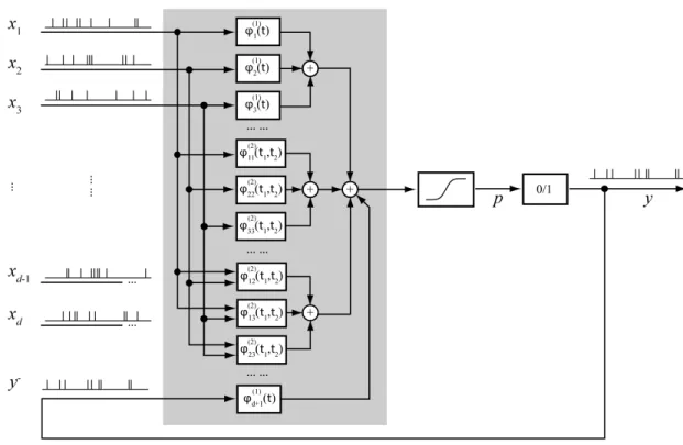
be summarized in a diagram as depicted in Figure 2.5.
Assuming sufficient smoothness, all kernel functions can be approximated with basis functions. Laguerre and B-spline representations are two popular choices. Song et al. [2013] compared both basis functions and suggested that B-splines provide a better approximation when characterizing local sparsity.
2.3.2 Kernel Functions and Basis Functions
B-splines, as described in detail in Schumaker [1980] and de Boor [2001], are piecewise polyno-mial curves and are commonly used for smoothing purpose thanks to their flexibility (where the desired degree of smoothness can be achieved by the appropriate choice of order and placement of knots) and the availability of computationally stable, inexpensive algorithms. Let B1(τ ), . . . , BJ(τ )
be a sequence of B-spline basis functions with certain degrees, say b, and fixed interior knots on [0, M ].
Figure 2.5: Second-order Volterra model with d inputs and one output. Inputs are convoluted with ϕ functionals of first- and second-order. The history of output y is treated as an additional input.
The kernel functions in (2.4) have the following approximation in terms of B-spline basis
ϕ(1)i (τ ) ≈ J X j=1 αj(i)Bj(τ ) (2.5) ϕ(2)i1,i2(τ1, τ2) ≈ J X j1=1 J X j2=1 α(i1,i2) j1,j2 Bj1,j2(τ1, τ2) (2.6)
where Bj1,j2(τ1, τ2) = Bj1(τ1)Bj2(τ2) is the product of two one-dimensional B-spline basis
func-tions. Plugging both approximations (2.5) and (2.6) into (2.3) yields the following approximation for Φ−1(θ(t)) Φ−1(θ(t)) = α0+ d+1 X i=1 J X j=1 α(i)j Z M 0 Bj(τ )dNxi(t − τ ) + d X i1=1 d X i2=1 J X j1=1 J X j2=1 α(i1,i2) j1,j2 Z M 0 Z M 0 Bj1,j2(τ1, τ2)dNxi1(t − τ1)dNxi2(t − τ2) (2.7)
where α0 = κ0. We further write ξj(i)(t) = Z M 0 Bj(τ )dNxi(t − τ ) ξ(i1,i2) j1,j2 (t) = Z M 0 Z M 0 Bj1,j2(τ1, τ2)dNxi1(t − τ1)dNxi2(t − τ2).
Consequently, (2.7) can be written as
Φ−1(θ(t)) = α0+ X(t)Tα (2.8)
where X(t) = (ξ1(1)(t), ..., ξJ(1)(t), ..., ξ(d+1)J (t), ξ1,1(1,1)(t), ..., ξ(d,d)J,J (t))T is a row vector and α is vec-tor of the corresponding coefficients of X(t). Furthermore, X(t) can be decomposed into two subvectors, namely X1(t) and X2(t), where
X1(t) = (ξ1(1)(t), . . . , ξJ(1)(t), . . . , ξJ(d+1)(t))T, X2(t) = (ξ1,1(1,1)(t), . . . , ξJ,J(d,d)(t))T.
Note that X1(t) and X2(t) correspond to the first-order and second-order kernels respectively.
2.3.3 Likelihood and Parameter Estimation
In this section, we consider likelihood based approach for parameter estimation in (2.7). For the ease of our notation, all input signals are considered as fixed. For the binary output signal y(t), observations are recorded at t = δ, 2δ, . . . , nδ. Here, under conditional independence, the likelihood function of y = (y((m + 1)δ), . . . , y(nδ))T given y(δ), . . . , y(mδ) can be written as
L(y|y(δ), . . . , y(mδ)) =
n
Y
s=m+1
P (y(sδ) = 1|y((s − 1)δ), . . . , y((s − m)δ))
=
n
Y
s=m+1
θ(sδ)y(sδ)(1 − θ(sδ))1−y(sδ), (2.9)
where θ(sδ) = Φ(α0+ X(sδ)Tα). Note that the likelihood function is a function of θ(t) and, as
a consequence of (2.8), is also a function of the unknown parameters α0 and α. In addition, the
log-likelihood function takes a form
n
The maximum likelihood estimators are denoted by (αb
M LE 0 ,αb
M LE). Maximizing the log-likelihood
function with respect to the unknown parameters is a well studied convex optimization problem with an iterative solution based on the Taylor series approximation of (2.10) or equivalently, the Newton-Raphson method or Fisher scoring [Givens and Hoeting, 2012]. It is worth mentioning that, unlike the logistic regression, these two methods are not equivalent for the probit link. In fact, Newton-Raphson method provides a faster convergence but requires the calculation of the Hessian matrix at each step (compared to the Fisher information). More details are given in Section 2.4.2.
2.3.4 Functional Sparsity and Neural Connectivity
In neural network, the neural connectivity is believed to be sparse in nature [Berger et al., 2005, Song et al., 2007]. In Tu et al. [2012], the authors defined two different types of sparsity. In particular, given multiple input neurons, only a small subset of these may have any relevance to the signal recorded from the output neuron. This property is referred to as global sparsity, and it should lead to the estimation of functionals ϕi corresponding to irrelevant inputs as zero. Among
the inputs that show relevance to the output signal, the impact will be limited in time, and the duration of the effect is often of interest. Outside of the interval in question, the functional will also be zero, which is referred to as local sparsity.
The classic maximum likelihood estimator (MLE) does not guarantee either sparsity, so a pe-nalized approach enforcing it is preferable. For parametric regression models, pepe-nalized approach has been widely studied and gained its popularity due to simultaneous parameter estimation and variable selection. Commonly used penalty functions include LASSO [Tibshirani, 1996] and SCAD [Fan and Li, 2001], group LASSO [Yuan and Lin, 2006] and group bridge [Huang et al., 2009]. In Wang and Kai [2014], the authors considered the problem of detecting functional sparsity for uni-variate, nonparametric regression models, and examined the performance of penalized approach
Figure 2.6: Top: A sequence of 13 cubic B-spline basis functions with 9 equally-spaced interior knots on the interval [0,1]. Bottom: An illustration of a function with local sparsity on interval [0,0.2]. There are 10 subintervals corresponding to 10 groups. On each subinterval, there are 4 basis functions coefficients taking positive values. For instance, to identify the sparsity of the function on [0, 0.1], all four basis functions (dashed line type) need to have coefficients zero.
with aforementioned penalty functions. In addition, these authors incorporated the group bridge penalty with an intuitive grouping method for estimating functions with global or local sparsities. For demonstration purpose, consider the function, shown as thick, solid line type in the bottom panel of Figure 2.6. Note that, except for some singletons, this function is zero on [0, 0.2]. In the top panel, a collection of cubic B-spline basis function with 9 equally-spaced interior knots are depicted. Approximating with these cubic B-spline basis functions, for sparsity on [0, 0.1], it is expected that the estimates for the coefficients of four basis functions, shown as dashed line type, are zero. Hence, it is natural to treat these four coefficients as a group. In general, for B-spline basis functions with degree b, each group consists of b + 1 coefficients.
In this paper, we adopt the grouping idea suggested by Wang and Kai [2014]. In fact, for the i-th first-order kernel ϕ(1)i (τ ) in (2.7), its coefficients of B-spline approximation in (2.5) can be assigned to J − b overlapping groups,
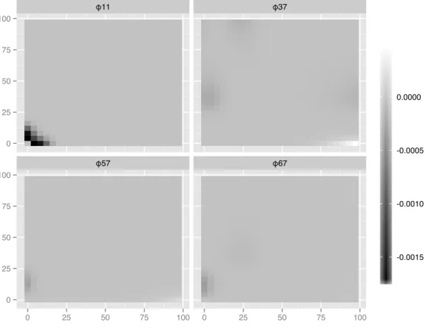
Similarly, for the second-order kernel ϕ(2)i1,i2(τ1, τ2), the grouping becomes rather complicated. Over
each small rectangle, spanned by two adjacent knots on τ1 and τ2, the sparsity can be determined
by (b + 1)2 coefficients. To be more specific, its coefficients of B-spline approximation in (2.6) can be assigned to (J − b)2 overlapping groups,
α(i1,i2) 1,1 . . . α (i1,i2) 1,b+1 .. . . .. ... α(i1,i2) b+1,1 . . . α (i1,i2) b+1,b+1 , . . . , α(i1,i2) J −b,J −b . . . α (i1,i2) J −b,J .. . . .. ... α(i1,i2) J,J −b . . . α (i1,i2) J,J For our convenience, we write the group penalty as
Pλ(γ)(α) = λ
G
X
g=1
|αAg|γ,
where G is the total number of groups and γ ∈ (0, 1) is a constant. Here αA1, . . . , αAG represent
the groups of coefficients as defined above.
Finally, the penalized log-likelihood criterion can be expressed as
l(α0, α) − Pλ(γ)(α) (2.11)
The penalized MLE is defined as the maximizer of this criterion. The computational aspects are covered in Section 2.4.4.
2.4 Computational Aspects with Big Data
2.4.1 Design Matrix
Write θ = (θ((m + 1)δ), . . . , θ(nδ))T. From (2.8), θ can be expressed as
Φ−1(θ) = α0+ Xα (2.12)
where the vector-valued function Φ−1is defined by applying Φ−1entry-wise. Here, X is the design matrix and can be written as X = (X((m + 1)δ), . . . , X(nδ))T.
The design matrix X can be represented as [X1, X2], where X1 and X2, based on X1(t)
and X2(t), correspond to the parameters of the first-order kernels and the second-order kernels
respectively. The elements of the matrix X1 can be calculated as
ξj(i)(t) = Z M 0 Bj(τ )dNxi(t − τ ) = X tik∈[t,t−M ) Bj(t − tik) (2.13)
for t = (m + 1)δ, . . . , nδ, j = 1, . . . , J and i = 1, . . . , d + 1. Here, tik are timestamps such that
input xi is taking value 1. The elements of the matrix X2 are derived using the formula
ξ(i1,i2) j1,j2 (t) = Z M 0 Z M 0 Bj1,j2(τ1, τ2)dNxi1(t − τ1)dNxi2(t − τ2) = ξ i1 j1(t) ∗ ξ i2 j2(t) (2.14)
Note that, the 2-dimensional B-spline basis functions are tensor products of the 1-dimensional linear basis. Consequently, the rows of X2 can be efficiently calculated as the Kronecker products
of the rows of X1. This observation is rather important for big data computation; in fact, the
matrix X2 does not have to physically exist, which largely alleviates storage and computational
challenges in further calculations.
2.4.2 Maximum Likelihood Estimation with Conjugate Gradient
The iteratively reweighted least squares (IRLS) is a well established algorithm for finding a maximum likelihood estimate of a generalized linear model (2.12); see McCullagh and Nelder [1989] for more details. This iterative approach is based on the Taylor expansion of the log-likelihood function using either observed or expected information. At the (k + 1)-st step, one finds the estimate of α, say α(k+1), based on the previously calculated α(k) by minimizing kW 1 2 k(z(k)− α0− Xα)k 2 2. Here, z
(k) is a current response vector and W
k is a matrix of weights
depending on α(k). In fact, Wk is a diagonal matrix with elements wj(k),
wj(k)= φ(α(k)0 + XTjα(k))2/(θj(k)(1 − θj(k))), (2.15) and z(k) is a vector with elements zj(k) defined as
where XTj is the j-th row of X, θ(k)j = Φ(α0+ XTjα(k)), and φ, Φ are the density and distribution
functions of standard normal respectively. Moreover, the minimization problem above has a closed form solution,
(α(k+1)0 , (α(k+1))T)T = (ZTWkZ)−1ZTWkz(k), where Z = [1, X]. In practice, for a moderately
large matrix X, the closed form solution at every iteration can be calculated using a map-reduce framework as described in Section 2.2.3. However, the operation of matrix inversion is not feasible with a massively large matrix X. An alternative solution is to use the conjugate gradient method. Conjugate gradient is an effective optimization method developed for solving quadratic op-timization problems of the type: min
x 1 2x
THx − xTb, but used also for more general nonlinear
optimization. It is based on the notion of conjugate vectors, say d1, ..., dp such that dTi Hdj = 0,
for i 6= j. The conjugate vectors are linearly independent and span the Euclidean space Rp. The solution of the quadratic optimization problem can then be expressed as a linear combination of these vectors. The coefficients of that representation can be obtained iteratively in p steps. The conjugate gradient method has been successfully applied to classification in the big data context due to its scalable computational complexity; see Komarek [2004]. In fact, the number of operations for a convex quadratic problem is estimated to be O(p). The implementation, which details can be found, among others, in Antoniou and Lu [2007], requires approximately p matrix-vector multiplications. To carry out the IRLS algorithm, at the (k + 1)-st step, the minimization problem can be expressed in terms of H = 2ZTWkZ and b = 2ZTWkz(k), where Wk and z(k)
are defined as in (2.15) and (2.16). Note that, in big data computation, the matrix H is never present in memory since it is only used in a matrix-vector multiplication, which is computable in a map-reduce framework; see Section 2.2.3. The vector b is of size p × 1 and it can be computed with map-reduce and stored in memory.
It is worth mentioning that conjugate gradient method is also flexible when additional linear constraints are present. For instance, in model (2.4), it is reasonable to assume that ϕ(1)i (M ) =
ϕ(1)i (mδ) = 0 for all first-order kernels. This can be effectively written as linear equality constraints in terms of the vector of coefficients. As pointed out by Antoniou and Lu [2007], the equality constraints result in the problem of dimension reduction, and the reduced parameter vector can be estimated following the same iterative procedure.
2.4.3 Penalized Maximum Likelihood Estimation
The MLE obtained using IRLS in Section 2.4.2 does not provide any sparsity. One way to enforce sparsity of the identified model is to consider minimizing the penalized log-likelihood as expressed in (2.11). The minimization problem poses computational challenge since it is non-convex. A popular approach is to approximate the log-likelihood function by a quadratic function. Let l0(α) = l(αb
M LE
0 , α) be the likelihood function after plugging-inαb
M LE
0 . The approximation of
l0(α) can be obtained via a Taylor series expansion at the maximum likelihood estimationαb
M LE; that is, l0(α) ≈ l0(αb M LE) +1 2(α −αb M LE)T O2l0(αb M LE)(α − b αM LE) where O2l0(αb
M LE) = −ZTWZ is the Hessian of the likelihood function evaluated at the
b αM LE, Z = [1, X] and W is a diagonal weight matrix. This quadratic approximation can be expressed as l0(α) ≈ l0(αb M LE) −1 2kW 1 2(z − Xα)k 2 2 (2.17) where z = Xαb
M LE. Thus, the penalized criterion (2.11) can be expressed as
argmin α 1 2kW 1 2(z − Xα)k 2 2+ P (γ) λ (α). (2.18)
In the special case of γ = 1, the penalty is essentially the LASSO penalty [Tibshirani, 1996]. For γ ∈ (0, 1), the optimization problem is non-convex, and Huang et al. [2009] provided an iterative solution that can be summarized as follows
2. For s = 1, 2, . . ., until convergence, compute α(s)= argmin α 1 2kW 1 2(z − Xα)k 2 2+ G P g=1 (ζg(s))1−1/γ P i:αi∈Ag |αi| where ζg(s)= cg(1−γτnγ)γ P i:αi∈Ag |α(s−1)i |γ, for g = 1, .., G
Note that each stage of the iterative procedure can be reduced to the minimization of a quadratic form with L1 penalty applied to the coefficients α. For small data set, it can be
efficiently solved by the LARS algorithm [Efron et al., 2004]. However, in the big data context, this algorithm may not be adaptable. Finding the solution to such a problem applicable to a large data set is the subject of the next section.
It is important to mention that the group bridge penalty described above can encounter stability issues in calculations [Percival et al., 2012]. An alternative approach is to use the SCAD penalty [Fan and Li, 2001], which can be written as
pλ(|αj|) ≈ pλ(|αb M LE|) + p0 λ(|αb M LE|)(|α j| − |αb M LE|) (2.19)
An analog of (2.11), equipped with SCAD penalty, can be expressed as 1 2kW 1 2(z − Xα)k 2 2+ G X g=1 pλ(kαAgk1).
Zou and Li [2008] proposed a one-step estimation procedure, which is based on a linear approxi-mation of the penalty function. Thus, (2.19) can be written as a standard LASSO problem; that is, 1 2kW 1 2(z − Xα)k 2 2+ G X g=1 ηgkαAgk1, where ηg = p0(kαb (M LE) Ag k1).
As will be seen in Section 3.2, in our application, the estimates using the group bridge penalty and the SCAD penalty are comparable.
2.4.4 L1 Regularization via Coordinate Descent Algorithm
As outlined in Section 2.4.3, parameter estimation with the group bridge penalty and SCAD penalty can be reduced to the LASSO problem. LASSO has an efficient implementation using a variation of the LARS algorithm [Efron et al., 2004], which is not well tuned for operating on the design matrix of high dimension. Another implementation was suggested by Friedman et al. [2007] and Friedman et al. [2010]. The elastic-net penalty, of which LASSO is a special case, can be computed by a coordinate descent and soft thresholding. The algorithm is applicable to linear models, or generalized linear models, in which case it can be integrated with the IRLS steps.
The idea of soft thresholding was proposed by Donoho and Johnstone [1995], and it was designed to recover a signal in the noisy environment by providing an adaptable threshold. This approach is motivated by a simple optimization problem
min
t
1
2(t − t0)
2+ λ|t|,
where λ > 0 and t0 is a fixed constant. The solution can be written as tmin = S(t0, λ) ≡
sign(t0)(|t0| − λ)+. This observation motivated the gradient descent algorithm for the LASSO
solution; see Friedman et al. [2010] for more details. In particular, starting from any given parameter values, one parameter is updated using the soft thresholding. The detailed algorithm is described in Friedman et al. [2010]. When implementing this algorithm, matrix-vector products are necessary and can be carried out efficiently under the map-reduce framework.
2.4.5 Tuning Parameters
The performance of parameter estimation relies on the choice of λ and γ. Here, the parameter γ is fixed at 0.5 following recommendations in Huang et al. [2009]. The common procedure for selecting λ is to proceed with model identification for multiple values of the coefficient and
1973], the Schwarz’ Bayesian Criterion [BIC; Schwarz, 1978], or, especially for larger models, the extended BIC [EBIC; Chen and Chen, 2008]. Such criterion-based methods are suitable for the selection in the first-order model, but more problematic for the second-order model, or for any large data in general. The selection of λ for the second-order model requires multiple identification efforts, but time cost, a major concern for big data analytics, does not allow an exhaustive search. In this paper, for the second-order model, we suggest to search for the tunning parameter among the predetermined increasing sequence of candidates starting from the value selected for the first-order model.
2.5 Data Analysis
2.5.1 Analysis of Neural Spikes
The data analyzed in this section comes from a public repository crcns.org and consists of neural recordings performed on a rat exposed to a maze; for details see Mizuseki et al. [2009a,b]. The data set contains timestamps of neural spikes (action potentials) recorded in eight neuron cells within a 90 minute timeframe. A portion of the data set, recorded over three seconds, is shown in Figure 2.7. All neurons come from CA1 region of hippocampus. We consider seven of them as inputs and one as output.
For each neuron, it is assumed that one observation, either 0 or 1, is recorded every δ = 1 millisecond (ms), which yields over five million observations. In addition, the memory length is chosen to be M = 400 milliseconds. Based on earlier studies [e.g., Song et al., 2013], the memory length is generally less than 1 second. In our data analysis, results from M = 400 and M = 1000 are very similar. For illustration purpose, we present only the results with M = 400 milliseconds. All the observations are used to fit the first- and second-order models described in the following subsections.
0 10000 20000 30000 40000 50000 60000 0 10000 20000 30000 40000 50000 60000 0 10000 20000 30000 40000 50000 60000 0 10000 20000 30000 40000 50000 60000 0 10000 20000 30000 40000 50000 60000 0 10000 20000 30000 40000 50000 60000 0 10000 20000 30000 40000 50000 60000 0 10000 20000 30000 40000 50000 60000
Figure 2.7: Three-second recording (out of 90 minutes) of seven inputs x1, . . . , x7 (top rows) and
output y (bottom row).
2.5.2 First-Order Model
In this section we model the probability of neural spikes as a GLM defined in (2.8) with a matrix Z = [1 X1] and its elements defined in (2.13). Even though the number of observations
n is over five million, the matrix X1 can be computed and stored in memory for all calculations.
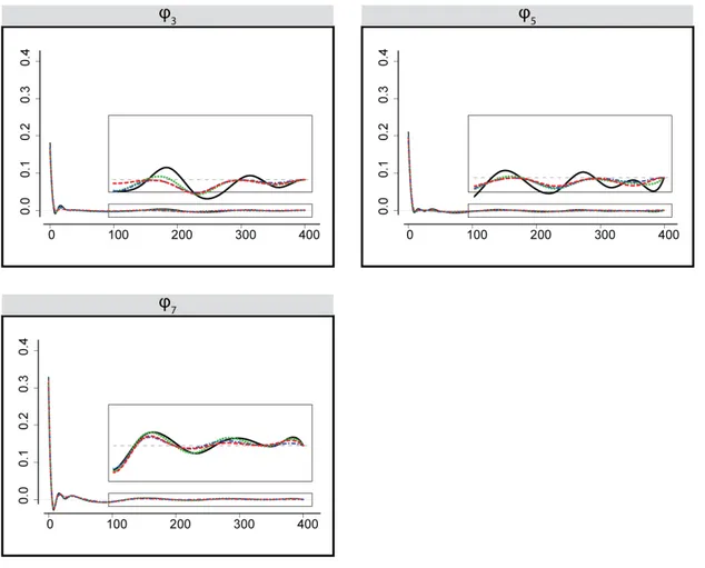
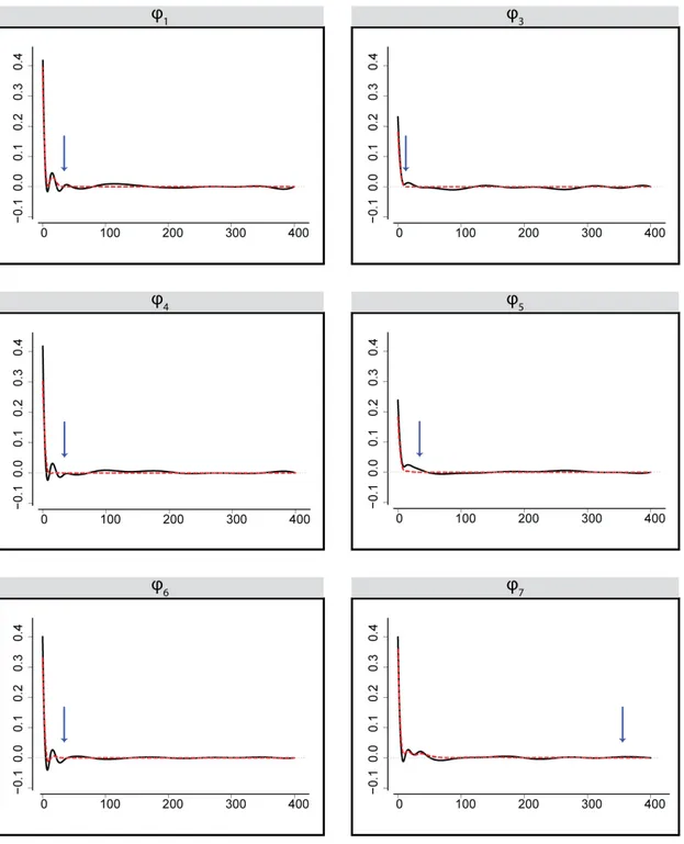
Here we assume that ϕ(mδ) = 0. We also consider a constraint ϕ(0) = 0 because the impact of the input spike is expected to have a positive delay. However, the delay might not be detectable in the data if the sampling rate is not high enough, in which case the value of the ϕ(0) may correspond to the maximum value of the functional. In fact, this turns out to be the case for all seven input neurons. Figures 2.8 and 2.9 show the results of the first-order model fit, with the MLE estimate depicted with a solid line, and three different penalized fits including group bridge (dashed), group SCAD (dotted) and LASSO (dash-dotted). The zoom-in view in each image shows the differences in sparsity estimation for all four models. The group bridge fit exhibits local sparsity in four out of seven neurons. The group SCAD and LASSO fits do not achieve the local sparsity in the examined range. The group bridge estimate was calculated with λn= 40 selected
Figure 2.8: Maximum likelihood estimation (solid) and penalized maximum likelihood estimation using a group bridge penalty (dashed), SCAD (dotted) and LASSO (dash-dotted) of ϕ functionals in the first-order model corresponding to the input neurons: x1, x2, x4, x6. The estimates are
Figure 2.9: Maximum likelihood estimation (solid) and penalized maximum likelihood estimation using a group bridge penalty (dashed), SCAD (dotted) and LASSO (dash-dotted) of ϕ functionals in the first-order model corresponding to the input neurons: x3, x5, x7. No sparsity is detected.
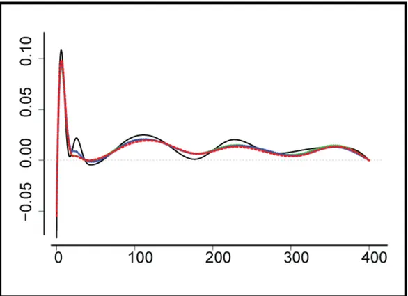
Figure 2.10: Maximum likelihood estimation (solid) and a group bridge estimation (dashed) of a ϕ functional in the first-order model corresponding to the output neuron. Local sparsity is not detected.
Figure 2.10 depicts the maximum likelihood and a group bridge estimation of the kernel corresponding to the feedback kernel. The negative value at 0 confirms the expected inhibitory effect of a recent spike on the probability of the immediate succeeding firing. The positive value close to 0 could be an indication of a clustering effect in neural spikes, which can also be observed in Figure 2.7. Local sparsity is not detected by any estimator.
![Figure 2.6: Top: A sequence of 13 cubic B-spline basis functions with 9 equally-spaced interior knots on the interval [0,1]](https://thumb-eu.123doks.com/thumbv2/5dokorg/5531672.144306/38.918.158.761.147.390/figure-sequence-spline-functions-equally-spaced-interior-interval.webp)