Analysis of phytoplankton adaptation to vertical water column mixing as indicated by primary productivity: data from the Potomac Estuary

ANALYSIS OF PHYTOPLANKTON ADAPTATION TO VERTICAL WATER COLUMN MIXING AS

INDICATED BY PRIMARY PRODUCTIVITY: DATA FROM THE POTOMAC ESTUARY

ARTHUR LAKES LIBRARY COLORADO SCHOOL OF MINES

GOLDEN, CO 80401

by

All rights reserved INFORMATION TO ALL USERS

The qu ality of this repro d u ctio n is d e p e n d e n t upon the q u ality of the copy subm itted. In the unlikely e v e n t that the a u th o r did not send a c o m p le te m anuscript and there are missing pages, these will be note d . Also, if m aterial had to be rem oved,

a n o te will in d ica te the deletion.

uest

Published by ProQuest LLC(2018). C op yrig ht of the Dissertation is held by the Author. All rights reserved.

This work is protected against unauthorized copying under Title 17, United States C o d e M icroform Edition © ProQuest LLC.

ProQuest LLC.

789 East Eisenhower Parkway P.O. Box 1346

of Science (Mineral Resource Ecology). Golden, Colorado Date / O / ( / ? Signed: 'ougla^C. Seedorf Approved: Dr. Ronald R.H. Cohen Thesis Advisor Golden, Colorado Date !

0

(! !<(£

Department Head, Environmental Science and Engineering

ABSTRACT

In an estuanne environment, differences in temperature and salinity between inflowing oceanic water and outflowing fresh water can make stratified layers. These layers can entrain phytoplankton for time periods that will allow them to adapt to a particular irradiance level. This will affect their physiology and be a driving force in their growth cycle. There are two general approaches to modeling the relationship of primary production to solar irradiance: those models which are empirical in nature and those which are rational. The data collected from the Potomac Estuary in 1984 and 1985 show a consistent photoinhibition effect when primary production is plotted as a function of light intensity. This makes it a good candidate for modeling with a rational equation that accounts for photoinhibition.

The maximum productivity (Pmax), half-saturation (Ks), and photoinhibition (Kj) coefficients from two rational equations were estimated for this data set using a Marquardt nonlinear parameter estimation routine that obtains least squares estimates of the coefficients which fit the data best. The objective was to establish whether they were related in a logical way to physical parameters that describe stratification and mixing in the water column.

The results from this study suggest that the physiological mechanism that controls phytoplankton’s ability to adapt their maximum productivity to variation in light intensity is faster than the mechanism that controls their ability to adapt to photoinhibition. Further, short-term adaption effects on maximum productivity are reflected in the Pmax coefficient and the long-term effects of photoinhibition are manifested by Kj. However, quantification of the relationship is not possible without a through understanding of the phytoplankton’s irradiance history. Therefore, traditional modeling of productivity experiments, which assume steady-state conditions, are inadequate to accurately describe dynamic systems such as the Potomac Estuary or the World’s oceans.

TABLE OF CONTENTS

ABSTRACT ... iii

LIST OF FIGURES...vi

LIST OF TABLES ... vii

ACKNOWLEDGMENTS ...viii Chapter 1. INTRODUCTION... 1 Chapter 2. LITERATURE R E V IE W ... 9 Chapter 3. METHODOLOGY... 16 3.1 Data Collection... 16 3.2 Calculations... 22

Chapter 4. RESULTS AND DISCUSSION...24

4.1 Data D escription... 24

4.2 Equation B eh av io r...34

4.3 Nonlinear Parameter Estimation... 40

4.4 1984 Results ...44

4.5 1985 Results ...49

Chapter 5. CONCLUSIONS... 54

REFERENCES C IT E D ...60

LIST OF FIGURES

Figure Page

1 Generalized Photosynthesis-Light C u r v e ... 4 2 Location Map of Piney Point Sampling Area on the Potomac River

and E stu a ry ... 8 3 Diagram of Box Incubator used for Primary Productivity Incubations . . . . 18 4 Productivity vs. Irradiance Curves for the Rectangular Hyperbola

Equation of Smith (1936).

K§ Held Constant - Pmax V ariable...35 5 Productivity vs. Irradiance Curves for the Rectangular Hyperbola

Equation of Smith (1936).

Pmax Constant - Ks Variable...36 6 Productivity vs. Irradiance Curves for Boulton’s (1979) Equation.

Pmax Ks Held Constant - Kj V a ria b le ...39

LIST OF TABLES

Table Page

1 Irradiance and Productivity Data 1984 - 1985 ... 25 2 Nonlinear Regression Analysis 1984 - 1985 ... 29

3 Density and Stability Data 1984 - 1985 31

ACKNOWLEDGMENTS

I would like to thank Dr. Cohen for suggesting this project and supporting me during the times when it looked like there might not be a viable outcome. Thanks also to Dr. Steve Maiinello and Frank Dunkle for serving on my thesis committee.

This thesis, as well as classes I took at Mines, benefitted from the conversations with many of my fellow graduate students in the ES Department. Therefore, my thanks to Judy B., Peter C., Michael C., Allison D., Denise D., Mike D., Susan F., Dan G., Bob H., Ed K., Andrea F., Cindy K. F., Robin M., Dan M., Roy and Carmen P., Theresa S. D. and Margaret S. I wish everyone the best of luck.

Finally, I would like to tip my hat to Texaco Inc. which provided funding for 99.9% of the thesis and classes at CSM. Texaco was also kind enough to provide the incentive for retraining; a blessing if ever there was one.

C hapter 1 INTRODUCTION

Phytoplankton are the source of energy that drives nutrient cycles in aquatic ecosystems and are the energy base for higher trophic levels. Phytoplankton are also a major source of dissolved oxygen in waters and a carbon dioxide sink; they respond very rapidly to nutrient inputs and are therefore key indicators of eutrophication. Moreover, phytoplankton productivity in the worlds oceans is now a topic of concern, because of the role it is thought to play in modifying the carbon dioxide content of the atmosphere and global climate change (Mann and Lazier, 1991).

Phytoplankton produce organic compounds from inorganic nutrients and light energy. The organic compounds made by the phytoplankton are called "primary production" and primary production per unit time per volume of water is called "primary productivity". The photosynthesis process consumes inorganic carbon and releases oxygen. Therefore, the rate of increase of oxygen in solution due to phytoplankton is a direct measurement of primary productivity.

In their natural environment, phytoplankton experience a wide range of irradiance that is related to such causes as diurnal and seasonal cycles in solar elevation, changes

in the weather, diffusion of surface light by waves, and turbulent transport of cells through the vertical light gradient (Marra, 1980a). In an estuarine environment, differences in temperature and salinity between inflowing oceanic water and outflowing fresh water can make stratified layers. These layers can entrain phytoplankton for time periods that will allow them to adapt to a particular irradiance level. The irradiance level that phytoplankton adapt to will affect their physiology and be a driving force in their growth cycle.

There are two general approaches to modeling the relationship of primary production to solar irradiance: those models which are empirical in nature and those which are rational. Empirical models are constructed with little regard to internal mechanisms and rely on a particular set of data to make quantitative statements about a system. In contrast, rational models are those which are built to describe the way components of the real system operate (Lederman and Tett, 1981). To be of any use in addressing the question of why phytoplankton adapt to a particular irradiance level, an equation which describes the photosynthesis-light curve should do more than tell us how the data points lie on the curve; the equation should ideally be heuristic and tell us about the physiology of the phytoplankton. For this reason, rational equations are preferred over empirical ones.

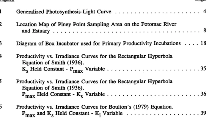
shown in Figure 1. The curve is frequently described by either empirical or mechanistic equations that generally contain two parameters (Jassby and Platt, 1976; Lederman and Tett, 1981). One parameter, Pmax> predicts the maximum specific rate

of photosynthetic activity that the phytoplankton are capable of during a specific set of conditions. The other parameter, Ks, is an irradiance value that describes the initial slope of the photosynthesis-light curve (Tailing, 1957a; Megard and others, 1984) and has its’ derivation from Minton-Miachelas enzyme kenetics. Since the parameters change in response to the environment, they can be used in a mechanistic equation to describe physiological changes that occur to phytoplankton in natural environments (Tailing, 1957a; Megard and others, 1984) or in laboratory cultures (Beardall and Morris, 1976).

Two of the more useful equations for modeling photosynthesis up to saturation take the form of a rectangular hyperbola. They are by Baly (1935):

P _{max A}x I P = (i) and Smith (1936): Ks + 1 P _max X I P = (2) (Ks2 + I2) /2

P m a x Z

o

CL

<

CL CL

PHOTOSYNTHESIS

VS.

LIGHT

AVAILABLE LIGHT

Figure 1. Generalized Photosynthesis-Light Curve. For low values of available light, the relationship is nearly linear. The slope of the curve is defined in part by the half­ saturation constant (Ks). For higher values of available light, the slope lessens until the dependent variable (primary production) attains an upper bound at the maximum productivity (Pmax). Further increase in light causes photoinhibition and the slope to become negative (Ki).

these equations is that they do not contain a parameter, Kj, that can adequately describe the curve if it moves into the photoinhibition range. Photoinhibition is defined as a characteristic light-dependent decrease in photosynthesis that occurs when the light level exceeds that which is necessary for the organisms to produce optimally (Powles, 1984; Neale and Richerson, 1987).

Equations which are mechanistic and treat photoinhibition are fairly scarce in the literature, but one such equation that may be applied to modeling phytoplankton growth at irradiances which include the photoinhibition range was found in an article by Roger Boulton (1979) on wine fermentation (R. Cohen, Pers. Commun., 1991). The equation discussed therein is a modification of the rectangular hyperbola proposed by Baly (1935) and Smith (1936). The equation was originally proposed by Haldane (1930) and has been used in a slightly different form by Peeters and Eilers (1978) and Senft (1977). Megard and others (1984) also used this equation in their study dealing with the effect of irradiance on the Pmax coefficient. The general form of the equation is:

where P, I, Pmax, and Kg are the same as described above and is a constant that accounts for inhibition at the highest irradiance levels. Note that P and I can be obtained

max

P = (3)

from field measurements, Pmax and Kg are estimated from the photosynthesis-light curve fitting procedure, and Kj can be calculated when a suitable curve is derived. While this equation has a term that accounts for inhibition, it does a relatively poor job of estimating real system values for Pmax and Kg because of the influence that the inhibition term (P/Kj) has on the equation. For this reason Equation 2 was used to estimate Pmax and Kg, while Kj was estimated from Equation 3.

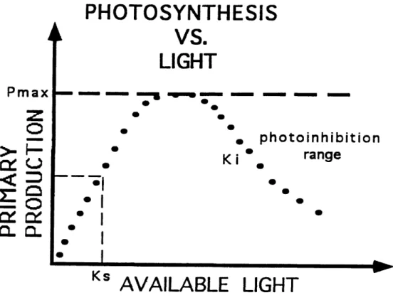
The basis of this study is primary productivity data that were collected from the Potomac River and Estuary in 1984 and 1985. The data were drawn from two locations along a transect across the Potomac (Fig. 2). These data show a consistent photoinhibitory effect when primary production is plotted as a function of light intensity. This makes it a good candidate for modeling with a rational equation that accounts for photoinhibition.

The main objective of this study was to examine whether the equation coefficients, Pmax, Kg, and as estimated from the productivity data were related in a logical way to physical parameters that describe stratification and mixing in the water column. The rational nature of the equation will tell us something about the physiology of the phytoplankton and how they adapt to various irradiance levels in a natural system. This is in contrast to most previous work which either relies on an empirically derived mathematical model that merely describes the photosynthesis-light relationship or uses

7 7 * SO*

PONT LOOKOUT J f

-1 0 I— i—S-— r1—

Figure 2. Tidal Potomac River and Estuary. Piney Point 6 (PP6) and 17 (PP17) are located along a transect adjacent to the Piney Point lab.

C hapter 2

LITERATURE REVIEW

Modeling primary productivity was first attempted by Arnold (1935), Burk and Lineweaver (1935), and Smith (1936). Early workers Riley (1946) and Sverdrup (1953) used linear equations for modeling photosynthesis. However, beginning with Tamiya (1951) and Tailing (1957a, b), authors began to concentrate on the ecological implications of fitting the more useful nonlinear models to photosynthesis data.

Authors who have reviewed mathematical equations that describe the photosynthesis-light curves of phytoplankton include Vollenweider (1965), Patten (1968), Jassby and Platt (1976), Platt and Gallegos (1980), Lederman and Tett (1981), Cohen and Church (1982), Chalker (1981), Cohen and others (1982), and Iwakuma and Yasuno (1983).

Platt and Gallegos (1980) summarized the modeling procedure for the photosynthesis-light relationship and concluded that up to five different parameters might be necessary to account for variations in field data. Jassby and Platt (1976) evaluated eight models in their summary. Lederman and Tett (1981) summarized the eight 2- parameter models discussed in Jassby and Platt (1976) and concluded that the minimum

and maximum number of parameters to adequately describe the photosynthesis-light relationship, while not considering photoinhibition, is two. This was in order to: (1) represent the way in which photosynthesis increases with illumination at low light levels and is not dependent on temperature; and (2) describe the saturation of photosynthesis at higher illuminations which is dependent on temperature.

Several workers have used a rectangular hyperbola equation to model productivity (Arnold, 1935; Baly, 1935; Burk and Lineweaver, 1935; Smith, 1936; Tailing, 1957a; and Eppley and Sloan, 1966). Other equations that include the inhibition of photosynthesis at higher illuminations have also been proposed (Steele, 1962; Vollenweider, 1965; Parker, 1974; Jassby and Platt, 1976; Webb and others, 1977; Lederman and Tett, 1981). Most authors are content to find an equation that will fit their field data. For example, Becacos-Kontos and Kontos (1981) used a simple cubic polynomial when other more conventional equations failed to describe their data.

To date, most of the models in use are purely descriptive in nature and do little to enhance the knowledge of the physiology of the phytoplankton (Platt and Gallegos, 1980). Those which do attempt to do more than simple description are generally only intended for the case ignoring photoinhibition. For example, Jassby and Platt (1976) concluded that the best equation for modeling primary production was their own hyperbolic tangent function. Unfortunately, it was only useful for data which show no

inhibition. In any case, the equation tells very little about phytoplankton physiology.

Lederman and Tett (1981) suggest that the ideal equation will have the minimum number of parameters necessary to describe the curve and that each parameter will correspond to a mutually independent well known physiological attribute. As a system becomes more well known, or as data collection becomes more precise, construction of rational models becomes easier. Unfortunately, ecologists are rarely able to use them because of the complexity of most natural systems. The authors conclude that the ideal is unattainable, or at least has not yet been attained.

More recent studies have used a modification of Jassby and Platt’s hyperbolic tangent equation (Neale and Richardson, 1987; Keller, 1989; Pahl-Wostl and Imboden, 1990) or have attempted using rational models that are based on enzyme kinetics (Peeters and Eilers, 1978; Aiba, 1982; Megard and others, 1984; Eilers and Peeters, 1988; Keller, 1989).

Scientists in the field of wine fermentation have been knowledgeable of substrate inhibition for many years (Hopkins, 1931; Hopkins and Roberts, 1935; Kunkee and Amerine, 1968; Vogt, 1970). A widely recognized equation for the specific growth rate of yeast where inhibition takes place after maximum growth rate is reached (Pirt, 1975; Boulton, 1979) is applicable to the growth rate of phytoplankton in light regimes that

include photoinhibition. The equation used by Boulton (1979), and originally derived by Haldane (1930), is a modification of the rectangular hyperbola form as proposed by Baly (1935), Smith (1936) and Tailing (1957a) for modeling the primary productivity of phytoplankton. This equation has the advantages of being relatively simple and based on physiological reality. This model or a variation has been used by several authors (Peeters and Eilers, 1978; Aiba, 1982; Megard and others, 1984; Eilers and Peeters, 1988).

Megard and others (1984) used Equation 3 to model productivity data taken beneath the ice of Como Lake, St. Paul, Minnesota during a span of five weeks in February-March of 1981. All of their samples were taken from the same depth to gauge the effects of irradiance and photoinhibition with changes in temperature. The calculations they made of photoinhibition were based upon estimates of Pmax and a term they specify as the "optimum irradiance." The authors suggest that without the assistance of nonlinear curve fitting their estimates are questionable. However, the authors conclude that: (1) photoinhibition decreases with an increase in temperature; and (2) adaptive changes of Pmax are very rapid. These conclusions are probably valid despite the questionable accuracy of their estimate values.

With a viable equation available to model phytoplankton productivity, investigation of vertical mixing and photoadaptation in water ecosystems may be

attempted. In natural waters, phytoplankton are exposed to wide variations in light intensity resulting from changes in the incident irradiation and transport vertically through the water column (Marra, 1980b; Falkowski and Wirick, 1981). Vertical transport consists of the interaction between turbulence and the cell’s sinking rate (Post and others, 1984). Therefore, the light to which an individual cell is exposed depends on the cell’s sinking rate and the mixed layer depth (Marra, 1980a).

Phytoplankton’s light-shade responses consist of changes in photosynthetic pigment, changes in enzyme activity, and changes in respiration, cell volume, and chemical composition (Falkowski, 1980). Adaptive phytoplankton types have been suggested by Steeman Nielsen and Jorgensen (1968). This work prompted Steeman Nielsen (1975) to conclude that the phytoplankton light-shade response is adaptive, whereas other workers (Yentsch and Lee, 1966; Beardall and Morris, 1976) have questioned whether the physiological responses to changes in light intensity are truly adaptive. They suggest that light-shade adaption is "more apparent than real" and that phytoplankton deep in the euphoric zone are "not physiologically up to par."

In a well-mixed water column it has been found that phytoplankton cells obtained at various depths respond to light in the same manner (Falkowski, 1980). This indicates that the mixing rates exceed the cells’ adaptation rate. In stratified water, cells that are high-light adapted have a higher photosynthetic capacity than their shade adapted

counterparts. This has led to the idea that vertical mixing can be inferred from knowing the vertical distribution of phytoplankton and their photoadaptive properties (Cullen and Lewis, 1988; Therriault and others 1990).

It has been found that recovery from photoinhibition depends on the duration and intensity of previous exposure (Critchley and Smillie, 1981; Powles and Bjorkman, 1982) and that the rate of recovery is slower than the rate of depression (Ohad and others, 1984; Greer and others, 1986). Neale and Richerson (1987) found in their study that phytoplankton previously photoinhibited had a higher threshold intensity for photoinhibition. Belay (1981) showed that phytoplankton could recover from severe photoinhibition within periods of less than 24 hours and that when the water column is stable, the population in the surface water adapts to become more resistant to photoinhibition. Lee and Vonshak (1988) found that there was a linear relationship between the specific rate of photoinhibition and the specific light absorption rate.

Vertical mixing has been found to introduce both random and deterministic short­ term variations in irradiance (Denman and Gargett, 1983; Neale and Marra, 1985). These variations have been modeled both experimentally (Jewson and Wood, 1975; Marra, 1978; Gallegos and Platt, 1981) and numerically (Platt and Gallegos, 1981; Falkowski and Wirick, 1981). Both types of models treat the possible effects of vertical mixing, but each approach has its own limitations as explained by Neale and Marra

(1985). Experimental models have difficulty in simulating realistic vertical mixing regimes because of the limitations created by the containment vessel while realistic biological responses are difficult to obtain from numerical models due to the complexity of those processes.

C hapter 3 METHODOLOGY

3.1 Data Collection

In 1984 and 1985, productivity data were measured using a light- and dark-bottle oxygen method as described by Greeson and others (1977), Cohen and Pollock (1983), and modified by Cohen while he was working for the USGS (Ronald R. H. Cohen, Verbal Commun., 1991).

Samples were collected from two locations (PP6 and PP17) along a transect across the brackish reach of the Potomac estuary adjacent to Piney Point (Fig. 2). Samples were obtained through an opaque tube by submersible pump from specific depths into 20-liter opaque, black carboys. This technique was used to minimize light shock to the phytoplankton.

A total of 25 samples were taken on 9 days to determine primary productivity, 12 drawn in 1984 and 13 in 1985. Samples drawn in 1984 were taken in June, October and November, and reflect either near surface (0.5 meters) or near water bottom depths (18.0 meters at PP6 and 7.0 meters at PP17). 1985 data were drawn in April, June, July, August and September, and reflect samples drawn from 0.5 and 4.0 meters for each

date in addition to 9.0 and 18.0 meters sampled in April and 9.0 meters sampled in September. All 1985 samples were taken from PP6.

The samples were decanted into incubation bottles within a light protected laboratory at Piney Point and were incubating typically within 30-60 minutes of sampling. Clear and opaque, black 300-mL B.O.D. bottles were filled by siphon from the 20-liter carboys. Prior to incubation, dissolved oxygen was measured in all the bottles with an Orbisphere polarographic oxygen probe; the B.O.D. bottles were filled to overflowing and then sealed to ensure that no oxygen bubble remained.

The filled bottles were placed in 92-cm wide by 122-cm long by 15-cm high wooden boxes (Fig. 3). The boxes were filled to overflowing with river water by submersible pumps such that the bottles were maintained at in situ Piney Point river temperatures. The boxes were divided into five sections by 2-cm high partitions. One section was exposed to full, surface sunlight. The other sections were covered by 1, 2, 3, or 5 layers of nylon screen transmitting 57-, 37-, 21-, and 8-percent of full surface light, respectively. Two opaque bottles for respiration, three clear bottles for full surface light, and two clear bottles for each light intensity were used for statistical purposes and to ensure reasonable results. The incubation bottles were shaken and rotated every hour to eliminate artifacts due to settling phytoplankton and sediment. Dissolved oxygen was measured at the end of the incubation period.

Figure 3. Diagram of Box Incubator Used for Productivity Incubations. River water, at in situ temperatures, flows through the hose into the incubation box; 100, 57, 37, 21, 8 are the percentages of surface light intensity as regulated by the number of nylon-mesh screens. The dark bottle is used for respiration measurements and is incubated under 8 percent light.

Samples for chlorophyll-a analysis were taken from the bottles at the beginning and end of the incubations. The chlorophyll-a concentrations were reported as averages of those measured at the beginning and end of the incubation. Chlorophyll-a normalization of the gross primary productivity is used so that specific rates are related to the active biomass. Normalization facilitates comparison between curves of light saturation. There are several possible choices for normalization including chlorophyll-a, particulate organic carbon, cell number and cell volume. Chlorophyll-a was used because it is fairly easy to measure in the field and has a good correlation among replicates (Platt and Gallegos, 1980).

Temperature and conductivity measurements of the water column were taken by a Hydrolab Multiparameter Surveyor concurrently with the productivity samples for later modeling of water density and stratification. Water density variations were quantitatively characterized by using Sigma-T, which is calculated as: (p - 1) x 1000, where p = water density, g/cm3. Water column stability was modeled using a variation of the Brunt- Vaisala Frequency (N2) (Henderson-Sellers (1984). The 1984 data generally consists of samples taken at 3.0 meter or less intervals down to the river bottom which was approximately 23.0 meters at PP6 and 7.0 meters at PP17. The 1985 samples were taken at regular intervals of 2.0 or 3.0 meters.

to the top of the Piney Point Lab that was connected to an HP Data Logger. Oxygen- based primary productivity was calculated from the light- and dark-bottle data using the following assumptions (Adapted from Cohen and Pollock, 1983):

1) Phytoplankton were the only source of oxygen in the sealed light bottles.

2) Community respiration (bacteria, phytoplankton, and zooplankton) was the only oxygen sink.

3) Phytoplankton respiration was the same in the light and dark bottles. Studies by Harris and Piccinin (1977) have suggested that light reduces phytoplankton oxygen consumption. Evidence concerning the effect of light on respiration is contradictory.

4) Phytoplankton respiration is constant with depth.

5) Phytoplankton productivity per unit of light in the afternoon is the same as in the morning. Lehman and others (1975) reported that productivity per unit of light in the afternoon is lower than that in the morning. Greeson and others (1977) recommend the use of Vollenweider’s method (Vollenweider, 1965) when incubations do not last for the entire dawn to dusk period. The method is based

on a plot of "percent cumulative productivity versus time", with sunrise to midday accounting for 56 percent of the daily productivity and midday to sunset representing the other 44 percent for a cloudless day. Cohen and others (1982), Schindler and Fee (1973) and Harris and Lott (1973) have suggested that the depression of productivity in the afternoon relative to the morning is an artifact of the productivity method and is associated with inorganic carbon depletion in bottles sealed from the atmosphere. Vollenweider (1965) suggests that reasonable day rate estimates can be obtained by assuming a symmetrical daily curve of instantaneous productivity rate. Therefore, for this data, partial day incubations were expanded to day rate integrals by assuming that instantaneous productivity followed the positive portion of a sine wave.

3.2 Calculations

Primary productivity, water column stability, and related parameters were calculated as follows: 1) R/Hj = i y N 2) Rd = R/HR X Dh 3) GPP/D = (Oa - C^) + Rj. 4) GPP/H = (GPP/D)/Dh 5) Sigma-T = (p - 1) x 1000 6) N2 = g x ---P2 - n p d2 - di (Brunt-Vaisala Frequency) 7) P = P _max x I (K 2 + I2)Vi (Smith’s, 1936 equation) 8) P = K s + I + (I2/Ki) (Boulton’s, 1979 equation) where: R/HR N

dark bottle respiration, in mg 0 2/L/h

total respiration for the entire incubation period, in mg 0 2/L duration of incubation, in hours

Dh Rd ° a ° b GPP/H GPP/D Sigma-T N2 P g d P I P.max K,

= hours of day light, in hours

= respiration during daylight hours, in mg O2/L

= concentration of oxygen at the end of the incubation, in mg o2/l

= concentration of oxygen at the beginning of the incubation, in mg O2 /L

= gross productivity per hour, in mg C^/L/h = gross productivity per day, in mg C^/L/d = water density, in (g/cm3 - 1) x 1000

= Brunt-Vaisala Frequency squared, in radians/sec = density, in g/cm3 = gravity, 9.8 meters/sec2 = depth, in meters = productivity, in mg O2/L n — irradiance, in /^Einsteins x 10

= maximum productivity constant, in mg O2/L

= half-saturation constant, in mg O2/L

Chapter 4

RESULTS AND DISCUSSION

4.1 Data Description

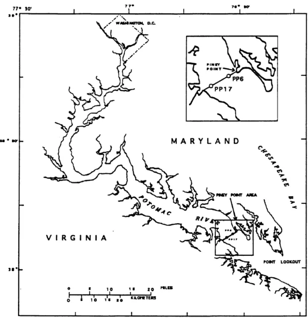
The productivity-irradiance data pairs that were collected from the Potomac Estuary during 1984 and 1985 form the basis for this study. The data is arranged by date, location and depth in Table 1. As discussed in the methods section, the irradiance is reported as ^Einsteins x 10^, and the productivity is in mg O2/L per mg chlorophyll-

a/L.

After collection and normalization with respect to chlorophyll-a, the productivity data were plotted vs. light intensity such that a curve-fitting computer program could be used to estimate initial guesses for the Pmax, Ks and Kj constants that would be used later in both Equation 2 and Equation 3. A Marquardt nonlinear parametric estimation routine was then utilized that takes the actual productivity-light data and compares it to the theoretical curves generated by the equations. The initial parameter estimates are used for the first iteration. The program then runs a series of iterations. Each subsequent iteration tries to better the curve fit to the data by minimizing the sum of the squares and thus making a better estimate of the constants (Table 2).

IRRADIANCE AND PRODUCTIVITY DATA 1984 - 1985

1984 DATA DATE LOCATION 1 P DATE... LOCATION 1 P

DATE LOCATION 1 ! p 10/3/84 PP8 10/11/84 PP8 6/6/84 PP8 18.0 M 2.75 84.45 0.5 M 2.25 61.46 18.0 M 4.25 173.1 2.75 91.39 2.25 63.59 4.25 203.87 7.2 159.27 5.9 117.75 10.8 270.98 12 161.64 5.9 122.38 10.9 276.81 12.85 189.41 10.35 142.45 19.1 308.07 12.65 220.89 10.35 143.87 19.1 308.07 19.5 198.69 15.9 154.86 29.45 348 19.5 211.1 15.9 180.31 29.45 370.86 34.3 114.93 28 111.82 51.7 221.93 34.3 121.88 28 137.18 51.7 285.16 10(3(84 PP17 10/11(84 PP8 6/6/84 PP17 0.5 M 2.75 147.46 18.0 M 2.25 82.51 0.5 M 4.25 240.41 2.75 149.58 2.25 62.51 4.25 264.9 12 246.39 5.9 115.31 10.9 301.77 12 275.95 5.9 122.16 10.9 318.88 12.65 297.41 10.35 128.36 19.1 359.69 12.85 339.76 10.35 138.63 19.1 383.72 18.5 302.72 15.9 140.71 29.46 383.78 19.5 316.91 15.9 158.52 29.46 392.04 34.3 188.46 28 87.11 51.7 224.19 34.3 178.63 28 98.38 51.7 252.51 10/3/84 PP17 10/11/84 PP17 10/3/84 PP8 7.0 M 2.75 116.8 0.5 M 2.25 71.2 0.5 M 2.75 113.81 2.75 124.78 2.25 76.05 2.75 118.6 7.2 185.53 5.9 132.43 7.2 182.78 12 165.53 5.9 138.1 7.2 193.98 12.65 215.58 10.35 156.09 12.85 250.81 12J5 234.57 10.35 168.85 12.65 257.56 19.5 203.4 15.9 168.33 19.5 239.78 19.5 203.4 15.9 178.74 19.5 253.61 34.3 100.83 28 128.29 34.3 154.77 34.3 118.94 28 131.85 34.3 202.88

Table 1. Irradiance and Productivity Data 1984 - 1985. Integrated daily solar irradiance (I) = /iEinsteins x 10^. Total gross primary productivity for the day (P) = mg O2/L

DATE LOCATION I P 1985 DATA DATE LOCATION 1 1 P 10/11/84 PP17 DATE LOCATION 1 P 4/3/85 PP8 7.0 M 2.25 72.32 4/3/85 PP8 9.0 M 2.05 23.94 2.25 72.32 0.5 M 2.05 21.7 2.05 24.13 5.8 143.78 2.05 24.33 3.3 32.72 5.8 151.33 3.3 37.18 3.3 33.85 10.35 145.89 3.3 28.04 5.35 39.34 10.35 185.36 5.35 33.88 5.35 43.81 15.8 174.02 5.35 33.88 9.48 53.01 15.9 174.02 9.48 57.86 9.48 56.07 28 115.28 9.48 59.42 14.6 51.09 28 115.28 14.6 53.64 14.8 56.07 14.6 59.8 25.8 42.11 11/8/84 PP8 25.6 44.45 25.6 44.37 0.5 M 1.85 83.27 25.6 45.62 1.95 85.28 4/3/85 PP8 5.15 133.54 4/3/85 PP8 18.0 M 2.05 18.53 5.15 140.29 4.0 M 2.05 23.25 2.05 18.23 9.1 159.08 2.05 24.64 3.3 22.37 9.1 161.21 3.3 27.36 3.3 23.08 14 151.26 3.3 34.55 5.35 32.04 14 151.26 5.35 38.07 5.35 32.04 24.6 103.3 5.35 44.75 9.48 38.37 24.6 103.3 9.48 58.36 9.48 40.52 9.48 57.2 14.6 35.75 11/8/84 PP8 14.6 58.53 14.6 38.32 18.0 M 1.95 68.7 14.6 59.8 25.6 25.54 1.95 76.41 25.8 48.28 25.6 28.09 5.15 118.06 25.6 49.22 5.15 122.78 9.1 125.58 8.1 143.23 14 122.7 14 128.73 24.6 80.2 24.8 91.87 Table 1. Continued

DATE LOCATION 1 1 1 P DATE LOCATION 1 P DATE LOCATION I P 8(13(85 PP8 7(17(85 PP8 9(19(85 PP8 0.5 M 3.45 76.81 4.0 M 3.58 119.88 0.5 M 2.8 75.83 3.45 82.07 3.58 148.73 2.8 77.09 8.18 133.83 9.5 258.85 7.45 167.25 9.18 145.26 9.5 259.3 7.45 167.82 18.15 188.59 18.8 305.58 13.2 200.44 18.15 202.13 18.8 312.71 13.2 211.72 24.8 213.36 28 282.04 20.3 228.9 24.8 218.29 28 322.72 20.3 235.39 43.6 131.03 45.55 121.88 35.6 225.87 43.8 168.03 45.55 152.18 35.8 243.7 8(13185 PP8 8(14(85 PP6 9(19(85 PP8 4.0 M 3.45 91.37 0.5 M 2.95 85.34 4.0 M 2.8 79.02 3.45 124.77 2.95 115.28 2.8 84.81 8.18 175.22 7.8 22223 7.45 180.97 8.18 181.54 7.8 228.27 7.45 198.8 18.15 233.55 13.75 328.35 13.2 218.31 18.15 235.5 13.75 330.8 13.2 220.98 24.9 232.5 21.2 380.17 20.3 242.58 24.8 239.18 21.2 380.98 35.6 164.02 43.8 163.8 37.2 334.42 35.8 208.03 43.6 195.53 37.2 354.25 9(16(85 PP8 7/17(85 PP8 8(14(85 PP8 9.0 M 2.95 37.89 0.5 M 3.58 103.94 4.0 M 2.95 70.81 2.95 65.89 3.58 105.07 2.95 94.38 7.8 159.48 9.5 218.82 7.8 150.74 7.8 172.24 9.5 221.79 7.8 158.72 13.75 205.2 18.8 272.74 13.75 190.4 13.75 211.58 18.8 278.23 13.75 214.35 21.2 252.22 28 311.09 21.2 202.92 21.2 277.48 26 317.72 21.2 224.24 37.2 237.64 45.55 235.24 37.2 139.88 37.2 238.06 45.55 255.44 37.2 189.4 Table 1. Continued

Our study found that using nonlinear regression analysis for Equation 3 to estimate Pmax, Ks and Kj constants introduced mathematical artifacts that resulted in artificially high values for Pmax. This situation has been encountered before by Jassby and Platt (1976) and Lederman and Tett (1981). Lederman and Tett further cautioned against estimating parameters in a nonlinear regression sequentially for the same reason. For these reasons Equation 2 was used to estimate Pmax and Ks. Only the inhibition constant (K|) was estimated using the Marquardt routine for Equation 3, and only then with the knowledge that the estimate was probably not a true reflection of the natural system.

Total irradiance values varied with weather and with the length of daylight on that day of the year. For this reason the constants were normalized with respect to the amount of irradiance measured on that day (Table 2). The normalized values were simply calculated by dividing the estimates by the total irradiance (in ^Einsteins x 10^).

Conductivity and water temperature data were converted to Sigma-T to quantitatively estimate water-column stability. Sigma-T is calculated as (p - 1) x 1000 where p = water density (g/cm3). Fresh-water dominated systems would generally have Sigma-T values around 10, whereas more oceanic dominated waters would cause Sigma- T values to approach or slightly exceed 20 (Table 3).

ARTHUR LAKES LIBRARY COLORADO SCHOOL OF MINES GOLDEN, CO 80401

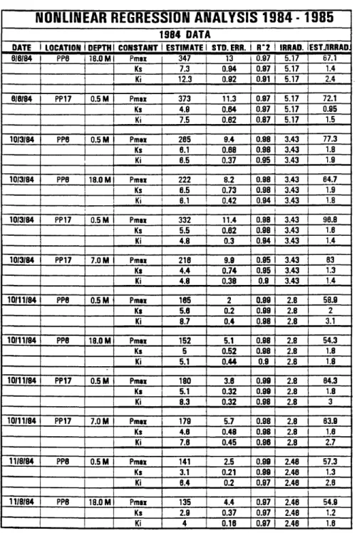
NONLINEAR REGRESSION ANALYSIS 1984 - 1985

1984 DATA

DATE 1 LOCATION DEPTH! CONSTANT 1 ESTIMATE! STD.ERR. i R*2 IRRAD. ESTJIRRAO.

818184 PP8 18.0M Pmax 347 13 0.97 5.17 67.1 Ks 7.3 0.94 0.97 5.17 1.4 Ki 12.3 0.92 0.91 5.17 2.4 6/0/84 PP17 0.5 M Pmax 373 11.3 0.97 5.17 72.1 Ks 4.8 0.64 0.97 5.17 0.95 Ki 7.5 0.82 0.87 5.17 1.5 10/3/84 PP0 0.5 M Pmax 265 9.4 0.98 3.43 77.3 Ks 6.1 0.88 0.98 3.43 1.8 Ki 0.5 0.37 0.95 3.43 1.9 10/3/84 PP8 18.0 M Pmax 222 8.2 0.98 3.43 64.7 Ks 6.5 0.73 0.98 3.43 1.9 Ki 6.1 0.42 0.94 3.43 1.8 I 10/3/84 PP17 0.5 M Pmax 332 11.4 0.98 3.43 98.8 Ks 5.5 0.62 0.98 3.43 1.6 Ki 4.8 0.3 0.94 3.43 1.4 10/3/84 PP17 7.0 M Pmax 218 9.9 0.95 3.43 63 Ks 4.4 0.74 0.95 3.43 1.3 Ki 4.8 0.38 0.9 3.43 1.4 10/11/84 PP8 0.5 M Pmax 185 2 0.99 2.8 58.9 Ks 5.8 0.2 0.99 2.8 2 Ki 8.7 0.4 0.98 2.8 3.1 10/11/84 PP6 18.0M Pmax 152 5.1 0.98 2.8 54.3 Ks 5 0.52 0.98 2.8 1.8 Ki 5.1 0.44 0.9 2.8 1.8 10/11/84 PP17 0.5 M Pmax 180 3.0 0.99 2.8 64.3 Ks 5.1 0.32 0.98 2.8 1.8 Ki 8.3 0.32 0.98 2.8 3 10/11/84 PP17 7.0 M Pmax 170 5.7 0.98 2.8 63.9 Ks 4.8 0.48 0.98 2.8 1.8 Ki 7.8 0.45 0.96 2.8 2.7 11/8/84 PP0 0.5 M Pmax 141 2.5 0.99 2.48 57.3 Ks 3.1 0.21 0.99 2.48 1.3 Ki 6.4 0.2 0.97 2.40 2.8 11/8/84 PP8 18.0M Pmax 135 4.4 0.07 2.48 54.9 Ks 2.9 0.37 0.97 2.48 1.2 Ki 4 0.18 0.97 2.46 1.0

Table 2. Nonlinear Regression Analysis 1984 - 1985. Pmax and Ks constants are estimated from the equation of Smith (1936). Ki constant is estimated from Boulton’s (1979) equation. Abbreviations are as follows: Standard error (STD. ERR.), total day irradiance (IRRAD.), estimate/total day irradiance (EST./IRRAD.).

1985 DATA

DATE LOCATION I DEPTH CONSTANT 1 ESTIMATE STD. ERR. R*2 I IRRAD. IEST./IRRAD.

4/3/85 PP8 0.5 M Pmax 64 4.9 0.92 2.58 25 Ks 6.2 1.1 0.92 2.56 2.4 Ki 0.4 0.52 0.92 2.58 2.5 4/3/85 PP8 4.0 M Pmax 64 2.5 0.98 2.58 25 Ks 5.8 0.53 0.98 2.58 2.3 Ki 9.7 0.45 0.98 2.58 3.8 4/3/85 PP8 9.0 M Pmax 58 1.8 0.98 2.58 22.7 Ks 4.8 0.37 0.98 2.58 1.8 Ki 7.6 0.27 0.98 2.58 3 4/3/85 PP8 18.0 M Pmax 40 1.3 0.97 2.56 15.8 Ks 4.3 0.4 0.97 2.58 1.7 Ki 5 0.16 0.98 2.58 2 8/13/85 PP8 0.5 M Pmax 234 8.9 0.99 4.30 53.7 Ks 11.2 1.1 0.99 4.38 2.8 Ki 15.4 1.2 0.94 4.30 3.5 6/13(85 PP8 4.0 M Pmax 250 9.4 0.98 4.36 57.3 Ks 7.8 0.92 0.98 4.38 1.8 Ki 13 0.71 0.97 4.36 3 7/17/85 PP8 0.5 M Pmax 338 4.5 0.99 4.55 74.3 Ks 11.3 0.39 0.99 4.55 2.5 Ki 13.4 0.49 0.99 4.55 2.9 7/17/85 PP8 4.0 M Pmax 327 11.1 0.98 4.55 71.9 Ks 7.8 0.84 0.98 4.55 1.7 Ki 5.9 0.52 0.9 4.55 1.3 8/14/85 PP8 0.5 M Pmax 450 13 0.99 3.72 121 Ks 14.7 0.87 0.99 3.72 4 Ki 17.8 0.81 0.99 3.72 4.7 8/14/85 PP8 4.0 M Pmax 230 9.8 0.98 3.72 61.8 Ks 8 0.98 0.98 3.72 2.2 Ki 14 1.1 0.95 3.72 3.8 8/19/85 PP8 0.5 M Pmax 250 4.4 0.99 3.58 70.2 Ks 8.5 0.39 0.99 3.58 2.4 Ki 28.4 1.3 0.99 3.58 7.4 8/18/85 PP8 4.0 M Pmax 259 9.2 0.99 3.58 72.8 Ks 7.7 0.7 0.99 3.58 2.2 Ki 18.5 1.2 0.97 3.56 4.0 8/19/85 PP0 9.0 M Pmax 314 25.5 0.98 3.58 88.2 Ks 13.6 2.2 0.98 3.56 3.8 Ki 18 1.4 0.97 3.58 5.1 Table 2. Continued

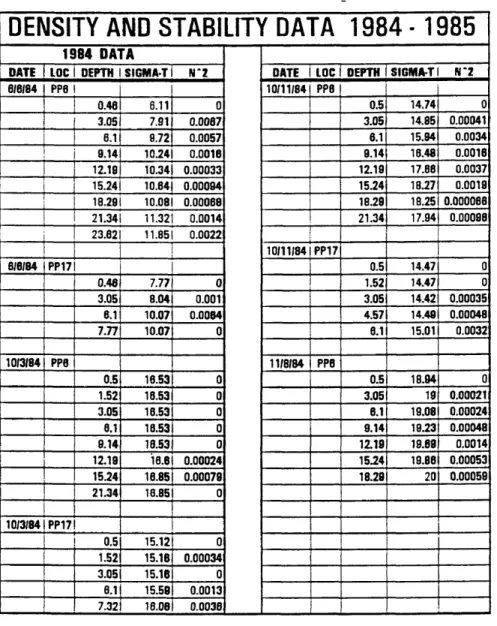
DENSITY AND STABILITY DATA 1984 -1985

DATE 1 LOC 1 DEPTH 1 SIGMA-T 1 N*2 DATE i LOC 1 DEPTH SIGMA-T I N*2

6/6/84 PP6 1 10/11/84 PP8 0.46 6.11 0 0.5 14.74 0 3.051 7.91 0.0087 3.05 14.85 0.00041 6.1 i 0.72 0.0057 6.1 15.94 0.0034 9.14I 10.241 0.0016 9.14 16.48 0.0016 12.19| 10.341 0.00033 12.19 17.88 0.0037 15.241 10.84) 0.00094 15.24 18.27 0.0019 18.291 10.081 0.00068 18.29 18.25 0.000088 21.341 11.321 0.0014 21.34 17.94 0.00098 23.62 11.851 0.0022 10/11/84 PP17 6/6/84 ppi7 i 0.5 14.47 0 0.46 7.77 0 1.52 14.47 0 3.05 8.04 0.001 3.05 14.42 0.00035 6.1 10.07 0.0084 4.57 14.49 0.00048 7.77 10.07 0 8.1 15.01 0.0032 10/3/84 PP8 11/8/84 PP8 0.5 16.53 0 0.5 18.94 0 1.52 16.53 0 3.05 19 0.00021 3.05 16.53 0 6.1 19.08 0.00024 8.1 18.53 0 9.14 19.23 0.00048 8.14 16.53 0 12.19 19.69 0.0014 12.19 18.8 0.00024 15.24 19.86 0.00053 15.24 16.85 0.00078 18.28 20 0.00059 21.34 16.85 0 10/3/84 PP17! 0.5 15.12 0 1.52 15.16 0.00034 3.05 15.16 0 8.1 15.58 0.0013 7.32 16.08 0.0038

Table 3. Density and Stability Data 1984 - 1985. LOC = Location, Depth is in meters, Sigma-T is calculated as (p-1) x 1000 where p is the water density, N^2 is the Brunt- Vaisala Frequency.

DATE LOC DEPTH SIGMA-T N-2 DATE LOC DEPTH SIGMA-T N‘ 2 ISIA5 5A1rA 4/4185 PP8 8114/85 PP8 i 14.84 0 0.5 14.31 0 4 14.89 0.00014 2 15.06 0.0048 7 14.7 0.000045 3 15.39 0.0032 10 16.36 0.0053 4 15.55 0.0015 13 18.48 0.0088 6 15.92 0.0018 16 19.02 0.0017 9 18.77 0.0027 19 19.71 0.0022 12 19.12 0.0075 22 19.98 0.00079 15 19.74 0.0019 18 20.24 0.0018 6113/85 PP8 0.5 11.63 0 8/15/85 PP8 2 11.8 0.00015 1 13.47 0 4 13.22 0.0078 4 15.79 0.0074 i 6 16.98 0.018 7 16.74 0.003 ! 9 17.92 0.003 8 18.23 0.0143 12 18.4 0.0015 I 10 18.43 0.00098 15 18.4 0 13 19.17 0.0023 18 18.4 0 18 20.17 0.0031 19 20.47 0.00097 6/14/85 PP8 23 20.47 0 1 12.87 0 4 15.23 0.0076 9/19/85 PP8 7 15.56 0.001 0.5 17.52 0 10 18.75 0.0038 2 17.85 0.0027 13 17.23 0.0015 4 18.54 0.0028 16 19.11 0.008 6 19 0.0022 19 19.28 0.00058 9 19.48 0.0015 21 19.89 0.0029 12 19.88 0.0012 15 20.22 0.0011 7/17/85 PP8 18 20.73 0.0016 0.5 14.12 0 21 20.73 0 2 14.12 0 4 14.83 0.0034 9/20/85 PPB 6 18.53 0.0017 1 17.72 0 9 18.58 0.0088 4 18.74 0.0032 12 19.88 0.0035 6 19.15 0.0013 15 19.91 0.00073 7 19.2 0.00048 18 20.52 0.0019 10 19.94 0.0023 13 20.17 0.00073 7/18/85 PP8 16 20.42 0.00081 1 13.63 0 19 20.45 0.0008 4 14.34 0.0022 21 20.45 0 7 16.88 0.0081 10 18.69 0.0058 13 19.88 0.003 18 20.32 0.0021 19 20.39 0.00024 21 20.39 0 Table 3. Continued

From the density and sampling depths, a variation of the Brunt-Vaisala Frequency was calculated for each increment measured. The Brunt-Vaisala Frequency, (N) or (N2), is the frequency in rad/sec of the oscillation that results when a boundary such as the pycnocline is displaced (Mann and Lazier, 1991). The Brunt-Vaisala Frequency is expressed as N where:

N = g x ---P2 ' P\

P d2 ' dl

Vi

g is gravity (9.8 meters/sec2), p is the density (grams/cm^), and d is the depth (meters). N2 (rad/sec)2 was used in this study rather than N because it is a better visual tool for indicating the relative stability of the water column between evenly spaced depth measurements (Table 3). N2, as the Brunt-Vaisala Frequency, has been termed the "stability parameter" by Henderson-Sellers (1984).

4.2 Equation Behavior

Equation 2 was used to estimate the Pmax and Ks constants for this data set. If the equation worked well, then Pmax would reflect the maximum productivity that the phytoplankton were capable of at saturation and the Ks constant would be the irradiance number at half-saturation. However, the very nature of the equation precludes Pmax from ever reaching its’ true maximum and the same for K^. Notice in Equation 2 below that irradiance functions as a multiplier of Pmax, whereas Ks lowers the Pmax value by being in the denominator:

^max x *

p = --- (2)

[Ks2 + F ]‘/2

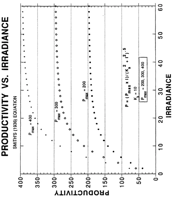
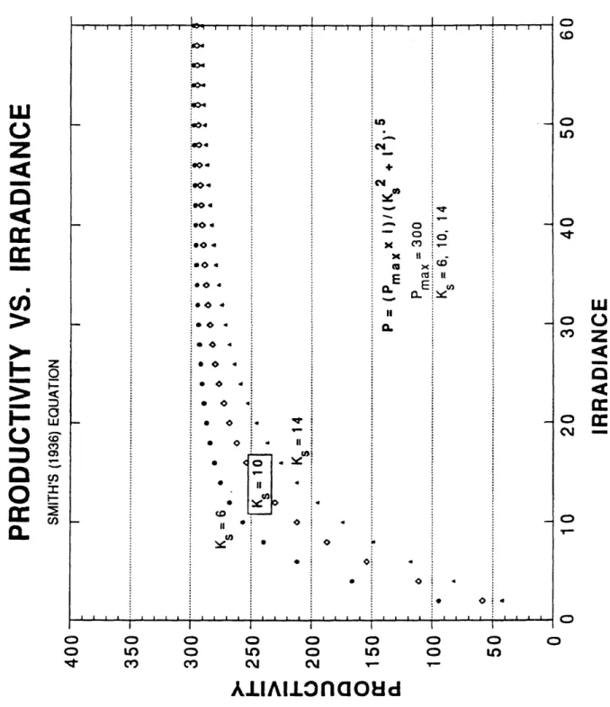
Figures 4 and 5 show the behavior of the curves generated by this equation assuming first in Figure 4 that Ks is constant at 10 and varying Pmax between 200, 300 and 400. The curves will eventually, at high enough irradiance, become asymptotic with the Pmax value. For the majority of this data set the irradiance was not high enough to achieve an asymptotic state. Figure 5 shows the nature of the curves while holding Pmax at a constant value (300) and changing Ks to 6, 10 and 14. Each curve will become asymptotic with the Pmax value of 300. However, Ks determines how quickly the curve will reach Pfflax.

P

R

O

D

U

C

T

IV

IT

Y

V

S

.

IR

R

A

D

IA

N

C

E

A i i A i i o n a o u d

Figure 4. Productivity vs. Irradiance Curves for the Rectangular Hyperbola Equation of Smith (1936). Ks Held Constant - Pmax Variable.

IR

R

A

D

IA

N

C

E

HI o

z

<

<

DC

CO

>

>

-o

o

DC

AiiAiionaoud

Figure 5. Productivity vs. Irradiance Curves for the Rectangular Hyperbola Equation of Smith (1936). Pmax Held Constant - Ks Variable.

IR

R

A

D

IA

N

C

E

Data analysis on the Kj constant was dependent on how Boulton’s (1979) equation works when the constants vary with low, medium and high irradiance. A critical look at Equation 3 while varying only the irradiance shows the following trends:

P x I r max A

p = --- (3)

Ks + I + (F/iq)

When the irradiance is very low Kj is insignificant, leaving P m a x and Ks to control the equation. At medium irradiance all three constants begin to factor in the shape of the curve. At high irradiance the inhibition term ( P / K j ) becomes the dominant term and controls the descent of the curve. The main problem with Equation 3 is that the inhibition term has an influence on the photosynthesis-light curve before saturation occurs. Megard and others (1984) have suggested that the mechanistic nature of the equation infers that photoinhibition does take place, even at the lowest irradiances. However, there is no field data or theoretical evidence to support this idea.

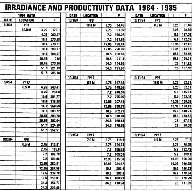
Before interpretation was begun, a sensitivity analysis of Equation 3 was performed similar to that done on Equation 2. The results are summarized in Figure 6. The analysis consisted of using typical values for the P m a x and Ks constants and then varying only the inhibition constant ( K j) . In Figure 6, P m a x and Ks were held constant at 600 and 30 respectively, while values were varied between 8, 10 and 12. The

equation takes the form:

600 x I p =

---30 + I + (P/Ki)

Inspection of Figure 6 shows that at low irradiance Kj will have a minimal affect on the curves as indicated by the similar initial slopes. The initial slope will continue as long as the I2/Kj term does not exert a strong influence on the equation. Larger values of Kj will therefore push the crest of the curve farther to the right. Notice that artificially high values of Pmax and Kg are necessary to bring the crest of the curve to a productivity value near 130.

P

R

O

D

U

C

T

IV

IT

Y

V

S

.

IR

R

A

D

IA

N

C

E

A i i A i i o n a o a d

Figure 6. Productivity vs. Irradiance Curves for Boulton’s (1979) Equation. Pmax and Kg Held Constant - Kj Variable.

IR

R

A

D

IA

N

C

E

4.3 Nonlinear Parameter Estimation

A nonlinear regression procedure obtains least squares estimates of the parameters in a nonlinear model. The program picked for this study uses a search algorithm to determine estimates that minimize the residual sum of squares. The algorithm was developed by Marquardt (1963), and is a combination of a straight linearization method and the method of steepest decent. Care was taken to choose initial estimates as close as possible to values that fit the actual system, otherwise another set of estimates could serve as a possible solution. The initial estimates were then optimized through the Marquardt iterative process.

Lederman and Tett (1981) showed in their paper that one of the major problems in nonlinear parameter estimation involves the order in which parameters are estimated. They found that when parameters are estimated sequentially the conclusions can be different than when the estimates are made simultaneously and independently. Further, they argued against any method other than direct simultaneous and independent estimation of the parameters based upon the occurrence of statistically biased numbers when other methods are used. To avoid these types of problems the Pmax and Kg parameters were estimated simultaneously using Equation 2.

When performing nonlinear regressions using Equation 3, it was found that if two or more of the constants were estimated at the same time, the results were inconsistent

with estimates made by subjective inspection of the data. The method most suited to this situation was to use the first approximations for Pmax and Kg and run iterations only on iq .

Acceptable values for each constant were based upon reasonable standard error calculations and R2 values. Standard errors varied for each parameter but were generally less than 1/10 of the estimated parameter for Pmax and Kj and less than 1/4 of the estimated parameter for K&. R2 values generally were greater than 90% (Table 2). A standard error that is 1/10 of the estimate means that the curve fit to the actual data is plus or minus 1/10 of the estimate number. For example, if the estimate for Kj was 5, then an acceptable standard error would be 0.5 or less. An R2 value of 90% means that the derived curve explains 90% of the variance from the actual field data. The difference between standard errors calculated for Ks and the other two constants appears to be related to the absolute value of the constant rather than an inherent mathematical problem.

To accommodate the rectangular hyperbola equation (Equation 2), the highest irradiance data was not used in the nonlinear parameter estimation routine. This was done to minimize the effect of inhibition on the Pmax and Ks parameter estimates. The data was then put back in for estimating Kj in Equation 3 (Table 2).

From an examination of the nonlinear regression analysis (Table 2), and comparison with the Sigma-T and N2 data (Table 3), an interpretation of the adaptive behavior of the phytoplankton can be made. Interpretation focused on the Pmax and Kj constants because Ks variations followed no discemable pattern.

Interpretation required several basic assumptions:

1. Phytoplankton adapted to higher irradiance will have higher Pmax and Kj values than their lower irradiance counterparts.

2. Irradiance levels decline in an exponential manner with water depth.

3. Phytoplankton sampled at a particular depth are representative of that depth.

4. The experimental procedure had the same effect on all samples.

5. Nutrient supply was not a major factor in photosynthetic efficiency. Evidence from Sakshaug and others (1989) and Cullen (1990) suggest that photosynthetic efficiency does not differ much as a function of nutrient supply. Conclusions by Tailing (1976) and Cohen and others (1982) suggest that CO2 depletion may

6. Phytoplankton species changes with time or depth did not significantly affect the productivity measurements.

7. Temperature changes did not significantly affect the productivity measurements. Megard and others (1984) showed in their study how Pmax was effected by changes in temperature. However, since these experiments were conducted at in situ temperatures, there should be no temperature related anomalies in the data.

4.4 1984 Results

Looking first at the data for 1984, Table 3 reveals that in June the water composition was fairly fresh with Sigma-T values ranging from 6 to nearly 12 at Piney Point Station 6 (PP6). The water stability data (N2) indicate stratification, especially in the upper 9.0 meters and the lowermost 3.0 meters. The data collected between 9.0 and 18.5 meters appears to be relatively more mixed. Note that the sample collected from 18.29 meters is a relatively less dense layer that has been trapped below denser waters.

The nonlinear regression analysis for June (Table 2) indicates that the Pmax values for 0.5 meters and 18.0 meters declined from 373 to 347. While a decline in the Pmax constant was expected to correspond to the decline in irradiance between the two depths, such a small drop indicates that the two populations of phytoplankton are similarly adapted to saturation levels of irradiance. The standard error calculations for the Pmax coefficients are nearly large enough to suggest little statistical difference between the values. The data on the inhibition constant (K^) is inconsistent with the expectation that the deeper sample would have the smaller constant corresponding to more inhibition. In this case the Kj constant actually increases with depth from 7.5 at 0.5 meters to 12.3 at 18.0 meters suggesting less inhibition with depth. The minimum change of Pmax and apparent reversal of Kj with depth from the expected trend may be explained by the low density layer that was trapped at about 18.0 meters depth. The fact

that there is a difference between how much the P m a x and Kj constants were affected may indicate that the physiology which controls the rates of adaptation that are manifested through the P m a x and Kj constants may be different. This possibility has been previously suggested by Lewis and others (1984), Cullen and Lewis (1988), and Therriault and others (1990).

The next series of measurements were taken during October 3, 1984 and consist of samples drawn from both PP6 and PP17 (Tables 2 and 3). Sigma-T and N2 values indicate a well mixed system for both stations. PP17 appears to be slightly fresher with Sigma-T values generally lower than PP6 and ranging from 15.1 to 16. The same depths at PP6 had consistent Sigma-T values of 16.5.

Nonlinear regression analysis for October (Table 2) indicates parameter estimate trends that coincide with predicted values for both the P m a x and Kj constant. At PP6 Pmax decreases from 265 at 0.5 meters to 222 at 18.0 meters, and at PP17 Pmax decreases from 332 at 0.5 meters to 216 at 7.0 meters. The discrepancy between absolute Pmax values between the two stations is probably due to different mixing rates. Kj varies at PP6 from 6.5 at 0.5 meters to 6.1 at 18.0 meters which is consistent with the idea that phytoplankton from a deeper depth will experience more inhibition when exposed to higher irradiance. However, the standard errors indicate that there may be no statistical significance between the two values. The Kj values from PP17 at 0.5

meters and 7.0 meters are both 4.8 which can be attributed to the rapid mixing which did not allow the phytoplankton to adapt to the different depths. The fact that there is a difference in Pmax values at both stations and no appreciable change in Kj suggests that the adaption up to and including saturation irradiance is faster than adaption to irradiance which may cause photoinhibition.

The density and stability data from October 11, 1984 (Table 3) suggest that the water column is considerably more stratified for PP6 than it was earlier in the month. N2 values below 3.0 meters down to 18.0 meters are about an order of magnitude higher than the values above or below these depths. Relatively more mixing occurs at PP17 which shows little change in Sigma-T and therefore low values of N2. Deeper data from PP6 as well as shallow data from PP17 indicate that there are some layers of relatively lower density that were trapped below other higher density layers. The influence of the more saline oceanic waters is becoming more apparent as indicated by Sigma-T values ranging from 14.5 to 18.

Nonlinear regression analysis for the October 11th data (Table 2) indicates that the layering allows the phytoplankton time to adapt to the particular irradiance better than the well mixed systems do. At PP6 Pmax values differ between 0.5 meters and 18.0 meters at 165 and 152 respectively. However, more of a significant difference is detected between the Kj values at 8.7 and 5.1 for the same depths. Pmax has an almost

insignificant drop from 0.5 meters to 7.0 meters from 180 to 179. Kj shows more difference, as it did at PP6, from 8.3 to 7.6. It is to be expected that the difference in Pmax values at PP17 would be small, but a much larger difference in Pmax values was expected at PP6 than what was estimated.

November density and stability data for 1984 (Table 3) indicate that the water system was dominated by oceanic water with Sigma-T values up around 19 and 20, while the stability factor (N^) indicated a moderately to well mixed water column.

The data from nonlinear regression analysis (Table 2) fit with the density and stability data in that Pmax and Kj decrease with depth as they would be expected to do.

Pmax decreases from 161 at 0.5 meters to 152 at 18.0 meters and Kj decreases from 6.4 at 0.5 meters to 4.0 at 18.0 meters.

An attempt was made for the 1984 data to normalize the constants in relation to the irradiance that occurred on that particular day. The normalization was accomplished simply by dividing the parameter estimate by the irradiance factor (Table 2). The normalized values for Pmax ranged from a high of 96.8 in October to a low of 54.3 for November. No definitive pattern emerged from this set of numbers save a tendency of the higher irradiance days to produce generally higher P max values, even after normalization. K s and Kj did not appear to be affected by either higher or lower

irradiance.

ARTHUR LAKES LIBRARY COLORADO SCHOOL OF MINES GOLDEN, CO 80401

4.5 1985 Results

For April of 1985 the density and stability data (Table 3) indicate a mixed water column down to 7.0 meters, a very strong gradient between 7.0 meters and 10.0 meters, and fairly stratified conditions below 10.0 meters to the bottom of the water column. Sigma-T numbers across the gradient indicate that a relatively fresh water plume overlies a cooler more saline layer that is mixing together very slowly.

Nonlinear regression analysis for April 1985 (Table 2) shows good correlation between the density and stability data and estimated Pmax and K- coefficients. The estimates for 0.5, 4.0 and 9.0 meters for Pmax are all in the same range. Pmax varies for these three depths from 64 for 0.5 and 4.0 meters to 58 at 9.0 meters. At 18.0 meters depth there is a dramatic drop in the Pmax value to 40. This drop in Pmax

records the crossing of the boundary layer that exists near 9.0 meters depth. Kj values are mixed over the upper three depths with values of 6.4, 9.7 and 7.6 respectively. The Kj value at 18.0 meters drops significantly to 5, again reflecting the boundary layer found near 9.0 meters. A possible explanation for the widely divergent Kj values in the upper three depths sampled could be that the phytoplankton are subject to intermittent surges of turbidity that are responsible for mixing the water column rather than a continuous mixing action. This would have the effect of allowing the phytoplankton to begin adaptation at a certain depth before a mass of turbulent water takes it to another level of irradiance. Since the Pmax constants appear to reach equilibrium more quickly,

they are all nearly the same value. Kj changes much more slowly and therefore has more variation.

The density gradient has a profound affect on the productivity of the phytoplankton; it is responsible for the lowest Pmax value (40) estimated for either 1984 or 1985. Mann and Lazier (1991) have suggested that phytoplankton and possibly nutrients would have a difficult time crossing barriers of this sort.

For the month of June, Sigma-T and N2 data (Table 3) indicate that stratified conditions begin at around 4.0 meters depth. 6/13/85 data indicate an abrupt boundary layer between samples at 4.0 meters and 6.0 meters where Sigma-T changes from 13.2 to 16.9 and N2 increases an order of magnitude. 6/14/85 data appear to be more mixed in general, but do have two medium strength density/stability changes between 1.0 and 4.0 meters and between 13.0 and 16.0 meters. The change between 1.0 and 4.0 meters is from a Sigma-T of 12.8 to 15.2 while the change at 13.0 to 16.0 meters is from 17.2 to 19.1.

The density/stability data discussed above would suggest that the constants estimated for these two depths would be very similar since there was fairly good mixing in the upper 4.0 meters. Pmax values were close at 234 and 250 for the two depths. However, Kj values were relatively more differentiated at 15.4 and 13.0 for 0.5 and 4.0

meters respectively. The more divergent Kj values may reflect the influence of the density/stability gradient that occurs very near 4.0 meters on the day of sampling.

For the month of July, density/stability data (Table 2) indicate that stratified conditions were prevalent beginning at 4.0 meters for both 7/17/85 and 7/18/85. Sigma- T values indicate that the influx of oceanic waters is increasing in relation to June’s values. Sigma-T varied over the water column in July from 13.6 to 20.4 whereas June’s Sigma-T numbers varied from 11.6 to 19.9.

Nonlinear regression analysis for July 17 produced estimates that correspond to the observed environmental conditions (Table 2). Pmax varied for 0.5 and 4.0 meters from 338 to 327, and Kj varied for the two sample depths from 13.4 to 5.9. Although the difference in Sigma-T and N2 values was not great between 0.5 and 4.0 meters for either day, the data suggests that the phytoplankton were entrained at those depths for a long enough period of time to cause a contrast in values.

The August 1985 data for stability and density is very similar to July’s (Table 3). Regular intervals of Sigma-T and high values of N2 indicate that the water column is stable and stratified. Sigma-T data for the water column vary over a range of moderately brackish (13-14) to fairly saline (19-20).

Regression analysis for August (Table 2) indicates that the samples taken at 0.5 and 4.0 meters have adapted to those depths. Pmax values are 450 and 230 for 0.5 and 4.0 meters respectively and Kj varies from 17.6 at the shallower depth to 14 at the deeper depth. The anomalously high Pmax value of 450 at 0.5 meters is difficult to explain. Even after normalization the value is still considerably higher than most values recorded for both 1984 or 1985. At this time no other explanation presents itself except natural variation.

Density and stability data for September 1985 (Table 3) indicate that the waters have a dominantly oceanic influence and are regularly stratified. Sigma-T values begin at 17 and vary to 20.7 while N2 values are relatively high especially on 9/19/85.

Nonlinear regression analysis is difficult to explain and problematic at best for September (Table 2). Pmax estimates appear to contradict the stratified water-column data that was collected at the same time. Pmax increases with depth from 250 to 259 and then to 314 for 0.5, 4.0 and 9.0 meters respectively; this trend is opposite from what is expected. Kj is less difficult to reconcile with values of 26.4, 16.5 and 18 for depths of 0.5, 4.0 and 9.0 meters. It is expected that the Kj values would decrease with depth. Why the 4.0 and 9.0 meter results would be similar is problematic. It is possible that the data is faulty or recorded incorrectly. It is unlikely that the regression analysis is bad since the results were rechecked to make sure of the procedure. Moreover, the standard

errors are acceptable and R2 values are excellent. If the data is taken at face value as a true representation of the conditions at the time of sampling, then this set of data would appear to violate one or more of the assumptions stated at the beginning of this section.

The 1985 data was normalized with respect to the irradiance which occurred on the day of sampling. As was the case for 1984, no definitive pattern was apparent for the data.

Chapter 5 CONCLUSIONS

These experiments were carried out in order to characterize the adaption behavior of phytoplankton at various depths and irradiance levels in a natural system. The first step was to select an equation capable of quantitatively evaluating the adaptive behavior of phytoplankton in relation to the water column in which they live. The hope was that the equation would give repeatable results that represented the natural system and would have a direct correlation with depth, density or stability.

Boulton’s (1979) equation (Equation 3) does an excellent job of fitting the productivity data. Unfortunately, the estimates necessary to fit the curve to the data have little basis in reality as was predicted by Jassby and Platt (1976) and Lederman and Tett (1981). What is left is an equation which is empirical in nature. The literature is full of empirical equations to model productivity; Jassby and Platt’s hyperbolic tangent function would probably serve as well or better than Equation 3 for describing the data. Since the point of the research was to quantify parts of the natural system, parameters which do not reflect this system were avoided.