Technical Trading Strategies
And the effect of trigger indicators
Paper within Master Thesis in Finance
Authors: Robin Ljungviken
Erik Lindquist
Tutors: Agostino Manduchi
Abstract
This thesis investigates whether technical trading rules, such as simple moving averages and trigger indicators, have a significant effect and can generate excess return against a simple buy and hold strategy. The rules will be applied on the OMX Stockholm 30 from the beginning of 2000 until the end of 2011. We also examine if the introduction of trigger indicators have a significant contribution to a dual simple moving average, in terms of return. The findings of the study were confirmed by an out of sample test. Re-sults conclude that no statistically significant excess return was generated from the use of technical trading strategies, when compared against a simple buy and hold strategy. The findings also submit that there are no statistically significant evidence, that the trig-ger indicators used would have a positive effect to the performance of the dual simple moving average.
Table of Contents
Abstract ...
Definition of terms ...
1
Introduction and Background ... 1
1.1 Problem Statement ... 2
1.2 Purpose ... 2
1.3 Previous research ... 3
1.4 Limitations of the study ... 5
2
THEORETICAL FRAMEWORK ... 6
2.1 Technical analysis ... 6
2.2 Efficient Market Hypothesis ... 7
2.3 Criticism against Efficient Market Hypothesis ... 8
2.4 High frequency trading ... 8
2.5 Technical indicators ... 9
2.5.1 Moving average ... 9
2.5.2 Simple moving average ... 10
2.5.3 Exponential moving average ... 10
2.5.4 Moving Average Convergence Divergence ... 11
2.5.5 Relative Strength Index ... 12
3
Methodology ... 13
3.1 Deductive approach ... 13 3.2 Collection of data ... 13 3.3 Quantitative method ... 13 3.4 Stock selection ... 13 3.5 Observation period ... 143.6 Selection of technical indicators ... 14
3.7 Assortment of parameters ... 15
3.8 Basic calculation procedures ... 16
3.9 Risk adjustment and statistics ... 17
3.9.1 Sharpe ratio ... 17
3.9.2 Jensen’s Alpha ... 18
3.9.3 Statistics ... 18
3.10 Transaction costs ... 19
3.11 Out of sample test ... 20
3.12 The Backtesting of data in practice ... 21
3.13 Limitations of the methodology ... 22
4
Empirical Results ... 24
4.1 Result from out of sample prediction ... 27
5
Analysis and discussion ... 29
6
Conclusion ... 32
6.1 Proposal for further research ... 33
6.1.1 Different parameters and strategies ... 33
References ... 34
Appendix ... 37
Definition of terms
MA – Moving AverageSMA – Simple Moving Average
Dual SMA – Dual Simple Moving Averages EMA – Exponential Moving Average RSI – Relative Strength Index
MACD – Moving Average Convergence Divergence EMH – Efficient Market Hypothesis
1 Introduction and Background
Technical analysis is a common expression for different techniques that seeks to fore-cast future stock prices, based on previous prices, and can be traced back to the 1600s. It was first used by Japanese businessmen when trading rice futures (Nison, 1994), in the late1800’s the Dow Theory (Brock, Lakonishok and LeBaron, 1992) was developed and nowadays hedge fund managers, investment banks and other financial institutes have computers that analyze the market data and executes trades that could last for less than a minute, this type of trading is known as high frequency trading (HFT).
By using technical analysis investors have been trying to predict and gain excess return on different markets around the world. Even though technical analysis is used by major banks, investment firms and for stock recommendations, the effectiveness of technical analysis is debated. Fama (1970) describes different conditions of market efficiency and concludes, among other things, that the weak-form of efficiency is strongly in support, which means that historical prices are fully reflected in current prices and should, there-fore, not allow any technical trading strategies to gain abnormal return.
Brock, Lakonishok and LeBaron’s (1992) published a frequently quoted article where they are testing technical analysis, such as different moving averages, applied on the Dow Jones Industrial Average Index. The article conclude that one could predict the market and gain abnormal returns with the help of technical analysis. Other articles that have been sucessfull in their use of tehnical analysis are Bessembinder and Chan (1995), Gunasekarage and Power (2001) and Metghalchi, Chang and Marcucci (2008) whom find evidence that technical trading have predictive powers and excess return in comparison to a simple buy and hold strategy, which simply means that you buy a secu-rity and hold it.
A study made by Hudson, Dempsey & Keasey (1996) find evidence that technical analysis may predict future price movements, but when considering transaction costs there is no evidence for excess returns generated from technical trading strategies. Malkiel (2005) argue that technical trading underperform in comparison to a simple buy and hold strategy, there was no evidence showing for predictive powers or that abnor-mal returns are generated when using technical analysis.
Since articles mentioned above have used tehnical analysis and reached mixed results when testing if one can gain excess return in different markets, it would be a contribu-tion to the area to investigate whether it is possible to generate abnormal return on the OMX Stockholm 30, and to study the actual effect of signal indicators.
Relative Strenght Index (RSI) and Moving Average Convergence Divergence (MACD) are among the most frequently used indicators (Torssell and Nilsson, 2000). Their sim-plicity makes them possible to replicate and suitable for the individual investor. That is also why these two indicators are chosen for this study.
This thesis tests two different indicators both individually, combined and by using dif-ferent parameters. The tests will be conducted on four difdif-ferent moving average lengths, which are also tested individually without indicators. The study is applied on data from 2000 until the end of 2011, divided into four sub periods for each company observed. The chosen index is the OMX Stockholm 30, mainly because of the lack of proper re-search, but also due to the authors’ interest in the Swedish market.
1.1 Problem Statement
The authors want to test whether technical analysis can allow the individual investor to gain abnormal returns in the Swedish stock market. We also want to conclude whether trigger indicators have a significant positive contribution.
1.2 Purpose
The purpose of this thesis is to evaluate technical analysis, from the individual investors view. Tested will be the effects of combining a dual simple moving average with the trigger indicators Relative Strength Index (RSI) and/or Moving Average Convergence Divergence (MACD) compared to only using a dual moving average, and to see wheth-er it is possible to gain abnormal returns on the OMX Stockholm 30 through these tech-nical trading strategies.
The authors will answer the following questions:
• Is it possible to gain abnormal returns by using dual moving averages and indi-cators, RSI and MACD, and thereby outperform the buy and hold strategy? • Can trigger indicators improve the performance of dual moving averages?
1.3 Previous research
A lot of research has been done in the area of technical analysis and technical trading rules, including the use of moving averages. When it comes to the trading rules using moving averages the majority of research are conducted in a similar way, meaning they are based on Brock, Lakonishok and LeBaron’s research, “Simple Technical Trading Rules and the Stochastic Properties of Stock Returns”. Brock et al (1992) are testing two of the simpler instruments in technical analysis; the moving average and trading range breaks at historical data from the Dow Jones Industrial Average index. Their tests conclude that technical analysis have predictive powers and are able to generate abnor-mal returns, at least when applied to the Dow Jones Industrial Average index using time series running from 1897 to 1986. Though there are no consideration of transaction cost, which may have significant impact at the final result.
Bessembinder and Chan (1995), Gunasekarage and Power (2001) are all using a similar approach when testing whether technical analysis may generate excess return. The dif-ference lies in the markets observed, the parameters and lengths used for testing the his-torical stock data. Gunasekarage and Power (2001) are testing on South East Asian Markets from 1990 to 2000 and Bessembinder and Chan (1995) are testing on Asian Stock Markets by using data from the mid 1970’s to the end of 1980’s. All articles above reached to the same conclusion, that stock price movements are predictable and technical analysis could be used for earning abnormal returns. Though it is observed that transaction costs might have significant effect for the final result when using tech-nical analysis.
Metghalchi et al. (2008) investigates the profitability of technical trading rules on the Swedish stock market between 1986 and 2004. Meghalchi et al (2007) concludes that, overall, the tested technical trading strategies are able to outperform the buy and hold strategy. Some of the trading rules showed at predictive powers as they were able to outperform the buy and hold strategy even when transaction costs were taken into con-sideration.
Hudson et al (1996) reach another conclusion when testing historical UK stock data from 1935 to 1994, technical analysis have some predictive powers when applied to da-ta sets over long time series, but due to transaction costs they where unable to observe that trading strategies based on technical analysis generate abnormal returns.
Lento & Gradojevic (2007) examines if technical trading rules are profitable and can outperform the buy and hold strategy on several North American indices. The results from the study are mixed and not significant or robust enough to conclude that all of these trading rules have an advantage compared to the buy and hold strategy. However, one must mention that some of the tested technical trading rules are of value when in-vestors are making decisions on financial markets. When costs are taken into account most of their trading strategies lose their statistical significance of generating excess re-turns.
Malkiel (2005) argue that active portfolio management such as technical analysis will increase the transaction costs and most likely decrease the performance of the portfolio. Mentioned in the article is that active portfolio management is a “loosers-game”, which will be outperformed by a simple buy and hold strategy.
Relative Strength Index (RSI) is the most frequently used counter-trend indicator. The idea is that the indicator is used to trade against the trend (Wong, WK., Manzur, M. and Chew, BK. 2003). Wong et al (2003) studied the Moving Averages (MA) and the Rela-tive Strenght Index (RSI) indicator to observe when they gave signal for when to enter-ing or exitenter-ing the market. Their test was conducted on stock data from the Senter-ingapore Straits Times Industrial Index from 1974 to 1994, divided into three sub-periods of sev-en years each. Whsev-en testing the MAs single, dual and triple MAs were used. Differsev-ent methods of using RSI were tested as well, but only the “crossover” method was reported (Wong et al, 2003). The authors concluded from the results that technical indicators could be useful and generate substantial excess returns. In general the single MA per-formed best, followed by dual MA and the RSI crossover method (Wong et al, 2003)
Chong and Ng (2008) studied whether the Moving Average Convergence Divergence (MACD) and the Relative Strength Index (RSI) were profitable on data from London Stock Exchange FT30 Index. The results show signs of predictability as both MACD and RSI outperforms the buy and hold strategy (Chong & Ng, 2008).
1.4 Limitations of the study
There are some limitations in this study. This section is to discuss the limitations and raise the awareness of those limitations, since they might have impact on the final re-sult.
• The study will put no emphasis in the bid/ask-spread since the authors where unable to retrieve historical bid/ask price for any of the chosen stocks during the observed time series. This might lead to an overestimated result as the more re-alistic approach would be to considerate a bid/ask spread, with lower net gain as a result.
• Stocks used for the study will be retrieved from OMXS30, consisting of the 30 most frequently traded stocks at the Swedish stock exchange. Companies that fail to exhibit complete stock data for the entire observation period will be ex-cluded.
• The study only intends to observe the effect of two different trigger indicators, Relative strength index (RSI) and Moving average convergence divergence (MACD). Other indicators may or may not perform better on the observed stock data in the study, however no other indicators will be taken into account.
• The moving average rule used in the study is constructed only from two simple moving averages holding different lengths. Other types of moving averages are thereby excluded.
• Through telephone interviews, the authors contacted four of the larger banks of Sweden (Danske Bank, Nordea, Swedbank and SHB) to receive an estimate of the historical commission costs for the entire time series. There were no evi-dence for when Internet trading became the most common way of trading stocks, still the commission used in the study will be entirely based at the Internet fee which if lower than the one we get if we make the trade at the bank. Also there are no emphasis put in the minimum cost for each broker. Due to this we will observe overestimated net gains in the result of the study.
2 THEORETICAL FRAMEWORK
2.1 Technical analysis
The concept of technical analysis is over 100 years old, examples of this is the Dow Theory (Brock et al., 1992) and the Japanese Candlestick Charts, which was first used when speculating in rice prices (Nison, 1994).
Technical analysis refers to many different techniques with the purpose of attempting to forecast future prices from past prices, or patterns. Both Brock et al. (1992) and Achelis (2001) state that past patterns have a tendency to repeat themselves. A basic assumption concerning technical analysis is; that since stock prices are based on supply and de-mand, which means that the major interest is in the market and its behavior. So instead of spending time trying to predict demand or looking at production costs the technical analyst can focus on finding trends and patterns (Kirkpatrick and Dahlquist, 2006) The other type of analysis, which is commonly known as the opposite of technical anal-ysis, is the fundamental analysis. While the technical analysis is primarily used for short-term investments, since it’s helpful predicting trends, the fundamental analysis is more used for long-term investments. This method focuses on finding mispriced stocks and predicting the value and the potential profitability of a security or a company based on earnings, P/E-ratios and other financial ratios (Bodie et al. 2011).
Even though technical analysis has been criticized for its potential to predict the future prices of the market (Malkiel, 2005), there are studies suggesting that not only could one predict future stock price movements using technical analysis, but also gain excess return compared to a simple buy and hold strategy. Metghalchi et al. (2008) and Chong & Ng (2008) are two examples of studies that emphasises positive performance of tech-nical analysis.
2.2 Efficient Market Hypothesis
To understand the significance of our thesis and the tests we will conduct, it is im-portant to describe the efficient market hypothesis (from here on referred to as EMH), developed by Eugene Fama (1970).
The EMH asserts that markets fully reflect all available information in security prices and thereby are efficient. When the markets are efficient and information is fully re-flected, securities will neither be over- nor undervalued, which means that one cannot expect any higher return than the one associated with the risk one are willing to take (Torssell, Nilsson, 2000).
The EMH consists of three different forms, or degrees, of efficiency. The Weak form of efficiency implies that prices fully reflect all information contained in historical prices, which would mean that the usefulness of technical analysis is rejected; Semi-Strong form implies that stock prices reflects both historical prices and all publicly available in-formation relevant to the market; The Strong form of EMH implies that all inin-formation known by any market participant is fully reflected in the prices (Malkiel, 1989).
Since EMH states that security prices fully reflect all available information (Fama, 1991), an important conclusion is that, even though there are some positive correlation in day-to-day price changes, it should not be possible to gain excess return through trad-ing systems since it would cause a too large amount of transactions which implies that even a small commission fee would hinder such an attempt (Fama 1970).
Malkiel (2005) claim that the robustness concerning the, alleged, predictable patterns is questionable. Malkiel (2005) also mention that the failure of most professionals should be evidence enough for market efficiency:
‘The strongest evidence suggesting that markets are generally quite efficient is that professional investors do not beat the market’ (Malkiel, 2005, p.2)
Malkiel’s (2003) conclusion is that, even if there are occational mispricing and anoma-lies in the stock market, those will most probably not last in the long-term due to the ef-ficiency of the market, in the end the belief of the stock markets efef-ficiency will not be abandoned. Lee & Yen (2008) draws a similar conclusion - beliving in the concept of efficiency and its continuing, important, role in markets.
2.3 Criticism against Efficient Market Hypothesis
In the late 1970’s and through the 1980’s the findings concerning EMH was mixed, though studies from authors such as Watts (1978) and Chiras & Manaster (1978) argues that there are signs of inefficiency. On the other hand, Jensen (1978) believe that there is no reason for abandoning the idea of efficiency. During the 1990’s and the beginning of the 21st century the challenger of EMH is the idea of behavioral finance (Lee & Yen, 2008).
Among others; Brock et al. (1992), Chong & Ng (2008), Gunasekarage & Power (2001) and Metghalchi, et al. (2008) finds evidence of some predictive powers when using technical analysis, these proofs makes the EMH questionable since, as mentioned earli-er, it should not be possible to predict future price movements.
However, the EMH cannot be rejected until it is proven that identified trends can be used to earn risk-adjusted excess return (Torssell and Nilsson, 2000).
2.4 High frequency trading
High Frequency Trading (HFT) is symbolized by a large amount of computer driven trades, that lasts from less than a minute up to a couple of hours, every day. The HFT trading holds a lower average return for each trade made. Due to volatile markets and overnight rate, High Frequent money managers usually reduce or eliminate their over-night holdings. These computer driven trades are taking advantage of occasional mis-pricing in the market, which pushes the markets towards efficiency (Aldridge, 2010). A high frequency trader is trying to go undetected when trading, by using a highly de-veloped computer system, but there is still a risk for errors and that’s why supervision from a human is important (Aldridge, 2010).
HFT can be done from all over the world and a large number of firms using it are locat-ed in cities with large stock exchanges, for example Chicago, New York, London and Singapore. This gives them the advantage to develop fast trading strategies (Aldridge, 2010). According to Aldridge (2010), the competitors in this business are mainly hedge funds, investment banks and independent proprietary trading firms. The use of a strate-gy based on High Frequency Trading is associated with high costs and advanced tech-nonolgy, therefore we do not consider it an option for the individual investor.
2.5 Technical indicators
2.5.1 Moving average
MA is the most commonly used instrument for technical analysis, the idea with MA is to identify a trend that could be used when trying to forecast future movement of a secu-rity. The method builds on a moving average of historical prices and is thereby a smoothing effect of the actual and more volatile security price curve. There are several different types of moving averages where the weights for historical prices are treated differently, mainly the difference between those are the weight that they put at the most recent data (Brock et al. 1992). The MA rule is a type of timing strategy and the per-formance of the model is often compared to a buy and hold strategy (Torssell, J. & Nils-son, 2000).
The calculation of MA reposes on an average of historical closing prices for the securi-ty. The length of the measurement periods vary depending on investors preferences for desired observation length, a long-term trend is often observed when measuring time se-ries between 100 and 200 days while popular time sese-ries for short-term trend often lies within an intraday average up to a 25 day time window. Time series in-between the long-term and short-term windows mentioned above are to be seen as intermediate lengths (Zhu, Y & Zhou, G. 2009)
According to the basic rules for moving averages, the idea is to look for crossovers, in most case one use dual or triple MA’s where different time series lengths are chosen. When those MA lines cross each other, signals are generated. The buy signal is ob-served when the short period average crosses above the longer period, and the sell sig-nal is generated when the short period crosses below the long period average (Torssell, J. & Nilsson, 2000). The MA rules are meant to exploit patterns in the security returns, this by giving a buy signal at the beginning of an upward trend, then investors are ex-pected to hold the security until a downward trend is identified where the MA rule gen-erates a sell signal.
2.5.2 Simple moving average
A simple moving average is constructed to assign all data points in the observation with same weights. It uses historical price data and creates an average by adding the desired length and then divides by the number of time periods.
!"#$%
! !
! = Simple moving average
Where n denote our chosen number of time periods while price is the closing price for the security (Achelis, 2001).
2.5.3 Exponential moving average
In contrast to a simple moving average that assign equal weight to all observations, the exponential moving average is placing larger weight to the most recent data and expo-nentially decrease the weight of earlier observations. EMA is included in the study since it is used when calculating the values of Moving Average Convergence Divergence. The weighting or smoothing constant assigns a number between 1 and 0 depending on the size of the sample; the value the weighting factor is given decides the importance of older observations. The larger the value the weighting factor is assigned, the more weight is put on most recent prices.
2
(𝑛 + 1)= 𝑆𝑚𝑜𝑜𝑡ℎ𝑖𝑛𝑔 𝑐𝑜𝑛𝑠𝑡𝑎𝑛𝑡
The smoothing constant is given by dividing two with n plus one, letting n denote num-ber of time periods (Achelis, 2001).
(𝐶𝑙𝑜𝑠𝑒! − 𝐸𝑀𝐴!)*W+ EMAy = Exponential moving average
Once the smoothing constant is given the exponential moving average could be calcu-lated. Given the above equation, Closep signify the closing price, EMAy is the
exponen-tial moving average of yesterday and W denote the smoothing constant (Achelis, 2001). Also for the first observation of the exponential moving average, let EMAy denote a simple moving average holding the chosen parameter length.
2.5.4 Moving Average Convergence Divergence
The MACD (Moving Average Convergence Divergence) indicator was developed by Gerald Appel, it is one of the most commonly used momentum indicators due to its simplicity to use. The model is basically built on moving average and measures a long-term MA against a more short-long-term one, the most common length is the 26-day EMA against a 12-day EMA. It shows how the moving average converges or diverges from the actual price trend. (Murphy, 1999)
The MACD line is generated when subtracting the 26-day EMA from the shorter 12-day EMA, while we get a signal line from creating a 9-day EMA of the MACD line. Once the two indicators are calculated they could be plotted next to a graph of the security price curve for easier interpretation. The basic formula used for calculating the MACD:
𝑀𝐴𝐶𝐷 𝑛 = 𝐸𝑀𝐴!(𝑖) ! !!! − 𝐸𝑀𝐴!(𝑖) ! !!!
here let x =12 while y =26 (Appel, G. & Dobson, E. 2008 and Achelis, 2001).
The benefit from using a MACD indicator is that it indicates both the trend and momen-tum for a chosen security. Different types of buy and sell signals will be generated when using the MACD indicator. Investors use the instrument differently depending on per-sonal preferences (Achelis, B. S. 2001).
As mentioned MACD could be used in several ways, two of them are to observe cross-overs or look for overbought/cross-oversold conditions. The most popular one is to look at the crossovers, a buy-signal is generated when the MACD line cross an goes above the sig-nal line while it is the opposite way around, a sell sigsig-nal is generated when the MACD line cross the signal line downward. The crossover technique could be used in the same way for when the MACD line crosses the zero line, either upward or downward. (Torssell, J. & Nilsson, 2000)
It is also possible to use MACD for indication of overbought or oversold conditions, if the short-term MACD diverge significantly from the longer-term MACD this may indi-cate that there are abnormal changes or swings in the security price, which should turn back to normal levels rather rapidly. The conditions and circumstances of overbought
and oversold properties vary from security to security and should be considered with caution. (Achelis, S.B. 2001)
2.5.5 Relative Strength Index
The Relative Strength Index (RSI) is a technical indicator compiled by Welles Wilder, J. (1978) a notable technical analysis. Welles Wilder published New concepts of nical analysis (1978), the issue came to be rather revolutionary for the process of tech-nical analysis. (Torssell, J. & Nilsson. 2000)RSI is used for measuring internal strength of a security, observing levels of overbought/oversold conditions.
Investors are free to use different lengths for the indicator but 14-day RSI is the most common and also advised length by Welles Wilder. Other popular lengths are 9-day and 25-day RSI where shorter time series foster larger volatility.
The RSI take ranges between 0 and 100. Let say that a 14-day RSI have a value of 100, this implies that the security had an ascending closing price the past 14 days while a value of 0 denote a declining closing price over the past 14 days. High values of the RSI claim that the security is overbought and low values that the security is oversold.
There are different ways for investors to use the RSI indicator, the methods used in this thesis will be further discussed in the methodology part.
100 − 100
1 + 𝑈𝐷 = 𝑅𝑆𝐼
Here U denotes the average of upward price change while D denotes average for down-ward price changes of the security. Since the RSI used for the study will be a 14-day pe-riod, ups and downs over a 14-day time series are used to calculate daily RSI values (Achelis, 2001).
3 Methodology
The study will be based on historical stock prices collected from the software DataStream. Sources reviewed for constructing the study lays mainly in financial arti-cles and previous research in the area of technical trading. The observations will be di-vided into three-year periods running between 2000-2011, the objective will be to measure the impact that trigger indicators have when applied to moving averages. The study will take brokerage cost into account for each transaction made, while there will be no regard to short selling.
3.1 Deductive approach
The paper will have a deductive approach since existing models and theory are used to ascertain that abnormal returns could be obtained from the use of technical trading in the Swedish stock market. We move from theory to empirics and the study intends to examine whether we can reject the hypothesis that technical trading does not generate abnormal returns in comparison to a simple buy & hold strategy.
3.2 Collection of data
The stock data used for studying how well moving average with trigger indicators per-form is collected from Thomson Reuters DataStream, the database provide adjusted stock prices where dividend payouts and stock splits are taken into account.
3.3 Quantitative method
The basis of the study lies in collecting and processing a large amount of data, therefore a quantitative method is substantial to make a significant analysis (Bryman, A. & Bell, E. 2005). We study whether a technical indicator based on moving average could gener-ate larger abnormal returns if combined with two different trigger indicators. Due to the large amount of data we need to process in order to conclude the study, we consider the quantitative method essential to make it manageable and synoptically
3.4 Stock selection
For stock selection the data sample chosen to observe are stock data consisting of OMXS30. By choosing OMXS30 we get a sample consisting of the most frequently traded stocks at the Swedish stock exchange. Furthermore we have divided the entire sample into four subsamples to get a better overview of how the methods perform
dur-ing different periods of time. Companies without enough stock data for the entire obser-vation period will be excluded from the sample.
3.5 Observation period
We collect the stock data using a time interval of 12 years for making our observations, the stock-data observations run from 1st Jan, 2000 to 31st Dec, 2011. The twelve year sample will hold four equally long subsamples, each consisting of three year stock data observations. Observations in the paper will be allocated with equal lengths to all sub-samples, this to enable a fair comparison of the subsamples.
Another alternative would have been to enlarge the number of periods to allow better isolation of stock cycles. Though this could decrease the statistical significance if some samples generate few signals during the shorter periods.
The four subsamples are consisting of the following periods: Period 1 (P1) 1st Jan 2000 – 31st Dec 2002 Period 2 (P2) 1st Jan 2003 – 31st Dec 2005 Period 3 (P3) 1st Jan 2006 – 31st Dec 2008 Period 4 (P4) 1st Jan 2009 – 31st Dec 2011
3.6 Selection of technical indicators
There are an abundance of available indicators concerning technical analysis, most of them based on historical stock data, where mathematical formulas are used to indicate signals whether to buy or sell the security. The indicators applied in the study will be simple moving average, MACD and RSI. Those indicators could be divided into sub-groups of technical trading. Where moving average and MACD are to be seemed as trend following indicators, measuring the trend to indicate when an upward (downward) trend is to await, hereafter the model generates a buy (sell) signal. The RSI on the other hand is a momentum indicator used for indicating a trend break.
Above indicators are applied in the study because of their simplicity to use for the pri-vate investor. Due to this, they are among the most popular indicators amongst technical analysts. (Torssell, J. & Nilsson. 2000)
3.7 Assortment of parameters
For the moving average we have chosen four different average lengths; [1,50], [20,50], [5,200] and [20,200]. The varieties of lengths depend on the fact that we want to scope the trend in different time perspectives measuring the effects both long-term and more short-term. Since the study aims at measuring the effects that trigger indicators have for the moving average, we are interested in seeing what impact could be found depending on the lengths of the MA.
The MACD indicator is constructed to use two different exponential moving averages (EMA), where the long period takes on an EMA of 26-days while the shorter one is re-flecting a 12-day EMA. There after the 26-day EMA is subtracted from the 12-day EMA, giving the MACD line. To generate a signal line a 9 day EMA of the MACD line itself is calculated.
To prevent whipsaws, the MACD model is constructed with a 1% band, which gener-ates a buy/sell signal first when we can observe the MACD line crossing the signal line by more than 1%.
When assorting the parameters for the Relative Strength Index, a 14-day RSI will be applied. The variety chosen for this indicator are to be found in the interval, where two different adaptation techniques of the RSI indicator will be used. The first method is called tops and bottoms; here we choose the interval [30,70], which show that a buy signal will be generated when the RSI moves below 30 while the model signals a sell signal when the RSI rises above 70.
The other method of using RSI will be to look at a centerline crossover [50,50] where we receive a buy signal when RSI falls below 50 while the sell signal is generated as RSI rises back above the 50 line.
For both methods of the RSI, the model are constructed with a filter that generates buy or sell signals first after three straight days holding the same signal are generated, this to reduce whipsaws.
To give the reader further understanding of the trading rules we will provide a definition of how to use them below:
SMA
If(SMA [1, 5, 20])>(SMA [50,200])=BUY If(SMA [1, 5, 20])<(SMA [50, 200])=SELL
RSI [30, 70] If(RSI [30,70])<30=BUY If(RSI [30,70])>70=SELL RSI [50] If(RSI [50,50])<50=BUY If(RSI [50,50])>50=SELL MACD If(MACD)>(SIGNAL LINE*0,01)=BUY If(MACD)<(SIGNAL LINE*0,01)=SELL
3.8 Basic calculation procedures
We use average daily returns to find how well the technical analysis perform in compar-ison to a simple buy & hold strategy. To find daily returns for each stock, we use the following formula:
𝑅! = 𝐿𝑁( 𝑃! 𝑃!!!)
Let Rt denote daily return for today while Pt stand for closing price of the stock today.
Average return for an observed period is given by the formula below: 𝑅 = 𝑅!
! !!!
𝑛
When measuring the total amount of risk which could be found when investing in the security, we choose to look at the standard deviation, where the following formula give us the risk for a chosen period of time;
𝜎! = √[1
𝑛 [𝑟 𝑠 − 𝑟]!
!
!!!
]
now let 𝜎! denote the risk or standard deviation, n the number of observations, r(s) our
observed stock return while 𝑟 indicate the mean return for our chosen time series.
3.9 Risk adjustment and statistics
3.9.1 Sharpe ratio
The Sharpe ratio is a risk measurement instrument that give the excess return or return in comparison to risk, thereby we classify it as a return-to-volatility measure. William Sharpe originally proposed the ratio thereby the name Sharpe ratio. It works so that it compares the investment in a chosen security to one made in a risk-free investment, it shows the excess return we get from every extra unit of risk we are prepared to take (Bodie et al. 2011).
The study will use the Sharpe ratio to measure the excess return earned for each extra unit of risk. The measurement is significant in order to make a risk-adjusted decision whether one should invest in a security or not. A negative Sharpe ratio would indicate that the portfolio or security is a non-rewarding investment choice.
𝑆𝑟 = (𝑟!− 𝑟!) 𝜎!
Here, subtracting the rate of the risk-free asset (𝑟!) from the mean return (𝑟!) of our portfolio, thereafter we divide the sum of this with the standard deviation of the portfo-lio (𝜎!) (Bodie et al, 2011). We get the risk-free rate from taking the logarithm for an average of the daily returns of a three month Swedish T-bill.
The Sharpe ratio gives the opportunity to measure the total reward to volatility trade-off. By using the Sharpe ratio we are able to receive a risk-adjusted performance meas-ure for different portfolios, which will be studied in this paper.
3.9.2 Jensen’s Alpha
Jensen differential performance index was first proposed by Michael Jensen (1968) the measure is also known as Jensen’s Alpha. It takes the average or mean return in com-parison to the return predicted by the CAPM model (Bodie et al. 2011). The model is used when calculating the alpha value for a chosen portfolio of assets.
Jensen’s Alpha is used and included in the study to get another risk-adjusted perfor-mance measure and see which stock should generate the largest abnormal returns. We use the following formula when calculating the measure:
𝛼! = 𝑅!− [𝑅!+ 𝛽!(𝑅! − 𝑅!)]
where 𝛼! denote the alpha value of the stock, 𝑅! the risk-free return, 𝑅! the return of
the market portfolio and 𝛽! is the beta value of the chosen stock (Bodie et al, 2011). 𝛽! = 𝜎!"
𝜎!!
Here retrieving the 𝛽! of the stock, for calculation 𝜎!! denote the variance of the market
portfolio, while 𝜎!" denotes the covariance between the stock and market portfolio (Brown. J. et al, 2011). Observed values for the market portfolio are received from Swedish OMX Stockholm 30 index.
3.9.3 Statistics
A two-tailed t-test comparing two samples will be conducted, the function will be con-structed in excel. Since the study aims to evaluate if it is possible to beat the buy and hold strategy by using moving averages combined with indicators, and if the chosen in-dicators can help generate a larger abnormal return than the dual moving average, a comparison of the mean returns will be performed.
𝑇 − 𝑣𝑎𝑙𝑢𝑒 = 𝑋!− 𝑋! 𝑆!!
𝑛!+𝑆!
!
𝑛!
Above formula was used for calculating the value of the t-test, where x1 and x2 both de-note the mean of the compared samples. 𝑆!! and 𝑆
!! stands for the two sample variances
The T-test will be used to evaluate the T-values at 5% and 10% significance levels. Since the study evaluate the statistical significance with two different T-tests, the au-thors will need diverse hypothesis for testing the statistical significance. The critical values observed is ± 1.96 at 5% and ± 1.645 at 10% significance level. (Aczel & Sounderpandian, 2008).
The first T-test is to observe any significant difference between the buy & hold strategy against the several methods based on technical analysis.
𝐻! = 𝑋!"− 𝑋!&! = 0
𝐻! = 𝑋!" − 𝑋!&! ≠ 0
here, 𝑋!" denote the mean return of the technical trading rule while 𝑋!&! denote mean return of a simple buy & hold strategy for the chosen security.
𝐻! = 𝑋!"− 𝑋!"#$ !" = 0
𝐻! = 𝑋!"− 𝑋!"#$ !" ≠ 0
The second T-test shown above is to investigate if there is any statistical significance for the dual moving averages when applying trigger indicators. 𝑋!" indicate the mean return when the dual SMA is combined with MACD, RSI or both. This compared to 𝑋!"#$ !" showing the return of the dual moving average.
3.10 Transaction costs
When making a study of technical trading where one are frequently trading securities, it is of high importance to take transaction costs into consideration to reach a more realis-tic outcome, since a large amount of transactions could reduce or even eliminate any excess profit. Isakov and Hollistein (1999) claimed that small or private investors are unable to benefit from excess profits when transaction costs are taken into account. When testing technical trading rules on the Swiss market, Isakov and Hollistein (1999) uses estimated transaction costs of 0.3% for financial institutes and 1.6% for the indi-vidual investor.
The transaction cost used for this study will be an average of the lowest possible com-mission available to an individual investor, offered by the largest Swedish banks or
bro-kerage firms. We find that the lowest possible transaction cost for a private investors have a percentage of 0,09%.
The following fees and commissions are to be found among the largest banks and bro-kerage firms in Sweden:
Name Percentage Minimum cost
Danske bank 0,10% 79 SEK
Avanza 0,15% 39 SEK
Swedbank 0,09% 99 SEK
Nordea - 99 SEK
SHB 0,09% 99 SEK
Nordnet - 99 SEK
In order to generate a more realistic result, only the brokerage firms having available historical commission for the whole observation period where used to get an average transaction cost. Swedbank and Danske Bank were the only firms with available histori-cal commission cost for the entire period, therefore an average consisting of commis-sion for each observed year were created. The generated commiscommis-sion that was used in the study got a value of 0,095%. This is significantly lower than the commission used in the study made by Isakov & Hollistein (1999) where a fee of 0,3% was requested for each transaction.
3.11 Out of sample test
To get a more accurate result the study will include out of sample tests, using five stocks from Swedish Large Cap, exluding stocks from OMX Stockholm 30, to conclude whether the method work for other stocks than those observed in the sample. There is a risk for data snooping when testing the same data over and over agin. By using out of sample tests, we test our strategies on not previously tested data. This should confirm our findings and see whether they are robust, if so, it should be possible to observe a similar result as the one in the original sample for the five companies tested. The meth-od that generates the largest amount of abnormal return, and show risk-adjusted
meas-urements that outperform the simple buy and hold strategy, will be used for evaluation in the out of sample test.
Randomly generated companies for the out of sample test are to be found in appendix (Table 2.9).
3.12 The Backtesting of data in practice
We based the whole simulation with the instruments chosen for the study in Microsoft Excel. For a start, the formula was calculating the number of buy and sell signals for the dual moving averages during a chosen time series. Buy signals were constructed to gen-erate the daily return of the tested security for that specific day. Once the signals was es-tablished for all four parametric values of the moving average, the data was filtered to observe how the signals occurred when combining the dual MA’s to the signals of RSI, MACD or even both parameters at the same time.
When combining two or more indicators the signals will most likely occur more sel-dom. This since the formula constructed for the study are built to wait giving a signal until both methods generate a buy signal. The sell signal on the other hand is generated once at least one of the indicators indicates for sell. This method will generate a larger amount false sell signals, though the authors consider it to be more safe to sell off if any of the indicators signals for a downward trend.
To measure the effect for the different indicator combinations and parameters an aver-age are created from the daily returns observed for each specific technique. In the same way the risk is measured for the days the model hold the security. With data collected from this result, risk-adjusted measurements such as the Sharpe ratio and Jensen’s alpha are created.
The Sharpe ratio is as mentioned earlier based at the calculated average return from each technique, subtracting the risk-free rate which is reflected by a daily average of a 3-month Swedish treasury bill. The sum of this divided by the standard deviation meas-ured, which stands as the risk measurement calculated in the model. Jensen’s alpha is constructed from the return series calculated above as well, which is then compared to the market portfolio, reflected by Swedish OMX Stockholm 30.
Once all companies observed in the study have been tested, an average is calculated to show which of the combinations perform the best during the observed period. The pa-rameter lengths that will be further tested in the study need to show good performance with abnormal returns from the start of the observation period. This since the authors considers the use of a single technique through the entire period to be more realistic. Once the combination performing best is found, further tests will be made by an out of sample test. The out of sample will test the most superior indicators and parameters at companies not included in the observed sample, using the same time series. The five companies that the out of sample will consist of are all gathered from Stockholm Large Cap. Once above results are compiled, two T-tests will be implemented to measure the statistical significance in the observed result. The first test will compare the techniques to a simple buy & hold strategy while the second test are to see if the trigger indicators have a significant effect for the dual moving average.
3.13 Limitations of the methodology
The study is based on investigating the largest stocks at the Swedish stock market, OMXS30. To generate an even more significant result one should include or at least consider observing a larger amount of stocks, besides it would be of interest to include more time series, longer and shorter over an extended period of time to see whether the result of the methods change and how great the impact is over time.
The trading strategy is based on closing prices of several securities, hereby it gets biased since no emphasis is put on the spread in opening/closing prices. The study would hold more reliable results if it was built on daily opening and closing prices. Except for the complexity of taking both opening and closing price into consideration, the main reason for excluding the opening price was because of missing data for some stocks during the observed time series.
When trying the methods of technical trading in the study, no emphasis is put on testing how the methods react to the use of short selling. We decided to take only long posi-tions due to different fees depending on the type of position we take.
The entire price data set is collected from Thompson DataStream, the study is thereby relying on the authentically of the price series displayed in the database. No missing
da-risk that occasional mistakes exist in the daily data for closing prices. Still Thompson DataStream is seemed to be a reliable source when collecting data, and any occasional mistakes are considered by the authors to have minor impact for the entire result.
When working in the software program Microsoft Excel there is also the risk of cor-rupted cells or formulas generating false observations, authors have taken this into ac-count by thorough observations of the all the formulas, further precautions are per-formed by making spot-checks of the stock data.
For calculating the Sharpe ratio and Jensen’s Alpha we need a measurement of the risk-free rate, there are different methods for obtaining Rf and the study are considering a 3M Swedish T-bill. Using any other parameter for receiving the risk-free rate might give a slightly different result.
The parameter values of MA are not specially optimized for the Swedish stock market, instead authors choose to use parameters that are proven to perform the best in other stock markets. Since the study aim to conclude whether the trigger indicators have a positive effect for MA or not - authors consider it more interesting to measure the con-sequences of triggers indicators during different MA lengths.
The authors chose to base the study fully at closing prices for each stock, due to absence of historical bid/ask price. The fact that no bid/ask-spread is included in the study create a bias since the closing price infrequently correspond to the actual bid- or ask-price. As some of the observed companies have insufficient data for the entire sample, the choice was made to exclude those companies to enable a full comparison between sub-samples of all stocks.
The following stocks listed at OMXS30 was excluded from the sample: • Alfa Laval B (ALFA)
• Lundin Petroleum B (LUPE) • Nokia B (NOKI SEK) • TeliaSonera B (TLSN)
4 Empirical Results
The following section will present results from the conducted tests; including return, risk, holding days and our risk-adjusted measurements. The results will be arrayed in chronological order to give the reader easier interpretation. The tables mentioned are to be found in appendix.
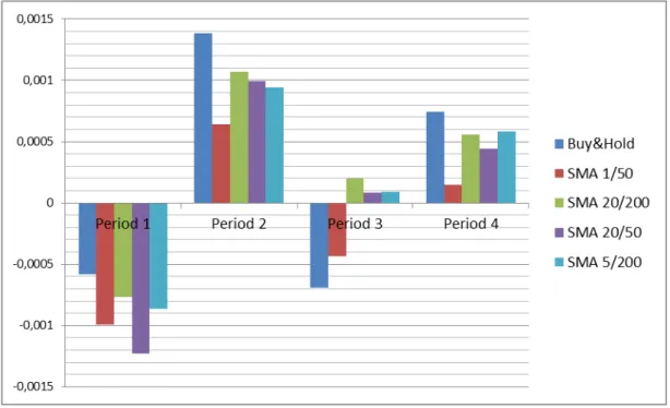
In the first period (table 2.1) the buy and hold strategy outperforms all of the dual mov-ing averages when not combined with a trigger indicator. We also measure a lower risk using the buy and hold strategy. The best performer of the dual moving averages was [20,200], which had a daily return of -0,0007675 compared to the buy and hold’s -0,00058287. The Sharpe ratio for the same parameters measure -0,0326 for the buy and hold and -0,03695 for MA [20,200]. Jensen’s Alpha favor the MA [20,200] strategy measuring -0,00088 while the buy and hold generates an alpha of -0,00092.
When introducing the indicator RSI (table 2.1) the best return for period one is provided by a technical trading rule, SMA [5,200] combined with RSI 50/50, which actually gen-erates a profit (0,00015) in contrast to the negative numbers provided by the buy and hold strategy (-0,00058). The second indicator, MACD, does not provide any positive value in terms of daily average return, instead its contribution is a decreased return. When combining both of the indicators with the dual moving averages the number of days holding the stock are very few and the daily average return is still negative. The best performance seen to the Sharpe ratio and Jensen’s Alpha is found in all lengths of SMA combined with RSI (with an exception for SMA [1,50] RSI [30/70]).
For the second period (table 2.2) the trading rule with dual moving average [20,50] combined with RSI [30,70] have the best performance. The trading rule outperforms the buy and hold strategy in terms of daily average return and when compared to the dual moving average, with the same length, it has an advantage. The MACD indicator, com-bined with any moving average length, cannot provide a better return than the buy and hold strategy or the dual moving averages.
When introducing the indicator above, SMA [20,50] combined with RSI [30,70], to the moving average, the Sharpe ratio, Jensen’s alpha and the standard deviation increases, and the number of days hold decreases.
The third period (table 2.3) presents the results from the tests performed during the third period. The buy and hold strategy has a negative daily average return, as well as the ma-jority of the trading rules. The strategy performing best for the third period is SMA [5,200] combined with the indicator RSI [50]. When only testing the SMA [5,200] the daily average return is positive, but when the indicator RSI [50] is introduced the daily average return increases. Two other moving average lengths combined with the same indicator also generate a greater daily average return when compared to the strategies using only moving averages, during the third period, where the majority of the returns are negative.
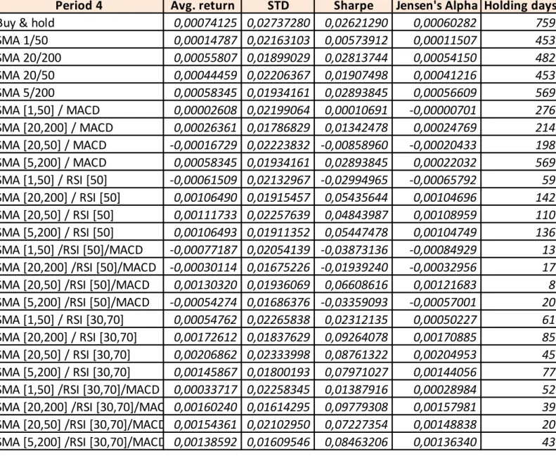
During the fourth period (table 2.4) the trading strategy SMA [20,50] combined with RSI [30,70] generated the highest daily average return and at the same time had the highest Jensen’s alpha, and the introduction of the indicator has a positive contribution on the return. The same strategy where also considered to be one of the riskiest strate-gies for the fourth period.
In terms of risk, the buy and hold strategy is showing the highest standard deviation for the fourth period. The majority of the tested strategies have a negative Jensen’s alpha, as well as a negative Sharpe ratio. The best performing strategy for this period has both a positive Sharpe ratio and a positive Jensen’s alpha.
The indicators RSI [50] and [30,70], combined with different moving averages, gener-ated higher return than the buy and hold, the moving average and the MACD indicators in general. A similar pattern goes for the Sharpe ratio, the majority of the two different RSI indicators have a higher Sharpe ratio as well as a higher Jensen’s alpha.
Another effect from the introduction of indicators, compared to only testing the moving averages, was a large decrease in number of days the stock was held.
The introduction of the different RSI indicators to the moving averages had a positive contribution in terms of return, but also slightly increased the standard deviation.
Tables 1.1 and 1.2 below are to display a summarized picture of how the technical trad-ing rules perform in comparison to the simple buy and hold strategy. For a clearer view of the result, please see appendix (tables 2.1-2.8).
Jensen's alpha/ B&H SMA
RSI [50] RSI [30,70] MACD SMA/RSI [50]/MACD SMA/RSI [30,70]/MACD
Period 1
25%
50%
0%
0%
75%
25%
Period 2
25%
100%
75%
0%
75%
75%
Period 3
100%
75%
50%
50%
0%
50%
Period 4
0%
75%
75%
0%
25%
75%
Displayed is the times that chosen indicator outperform the Jensen's Alpha value of the buy and hold strategy
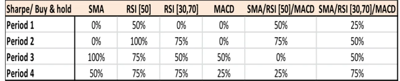
Table 1.1 The percentage displayed in table 1.1 above are reflecting the number of times that any chosen strategy outperformed the buy and hold strategy in terms of Sharpe ratio during the same time series. From observing the table we are able to determine that only two out of six methods are able to present a Sharpe ratio, which outperform the simple buy and hold strategy for all observed periods. The indicator performing best using the Sharpe ratio as a measurement is the RSI [50] combined with different lengths of SMA.
Table 1.2 The values in table 1.2 are reflecting the performance of each indicators Jensen’s alpha value against the alpha value of the buy and hold strategy. As seen above, only two of the six strategies perform better than the buy and hold strategy over the entire time se-ries observed. RSI [50] is still the indicator performing best against the buy and hold strategy.
All of the values obtained from the first t-test failed to reject the null hypothesis that the average return from technical trading strategies differ significantly from the average re-turn of a simple buy and hold strategy. This applies both at the 95% and 90% confi-dence interval, meaning that there are no significant difference of the returns from the buy and hold strategy and the different technical trading. Since all indicators failed to display values that allow us to reject the H0, none of the returns generated from
tech-Sharpe/ Buy & hold SMA RSI [50] RSI [30,70] MACD SMA/RSI [50]/MACD SMA/RSI [30,70]/MACD
Period 1 0% 50% 0% 0% 50% 25%
Period 2 0% 100% 75% 0% 75% 50%
Period 3 100% 75% 50% 50% 0% 50%
Period 1 Avg. return STD Sharpe Jensen's Alpha Holding days Buy & hold 0,00067832 0,02356926 0,02405541 ‐0,00092158 751 SMA [5,200] / RSI [50] 0,00055403 0,02208806 0,01228101 0,00041354 150
Period 2 Avg. return STD Sharpe Jensen's Alpha Holding days
Buy & hold 0,00079447 0,01663382 0,04395506 0,00096997 755 SMA [5,200] / RSI [50] 0,00096249 0,01366842 0,06578355 0,00085784 150
Period 3 Avg. return STD Sharpe Jensen's Alpha Holding days
Buy & hold ‐0,00019574 0,02304189 ‐0,01243585 ‐0,00056773 753 SMA [5,200] / RSI [50] ‐0,00113593 0,02024979 ‐0,06058012 ‐0,00122586 99
Period 4 Avg. return STD Sharpe Jensen's Alpha Holding days
Buy & hold 0,00061343 0,02455205 0,02401854 0,00060282 759 SMA [5,200] / RSI [50] 0,00047808 0,01732604 0,02622363 0,00045898 150
nical trading strategies are to be seen as significantly different from those of the buy & hold strategy.
The second t-test was constructed to test if the return gained from applying trigger indi-cators was significantly different from the ones only using a dual simple moving aver-age as a strategy. The result from this t-test was similar to the one testing technical trad-ing strategies against the buy and hold strategy, although the second t-test provided higher t-values, we still failed to reject the H0 hypothesis – meaning there are no evi-dence that the trigger indicators would have a statistically significant contribution.
4.1 Result from out of sample prediction
To see if the best performing strategy, in terms of return, Sharpe ratio and Jensen’s al-pha, could perform well in another environment than the one previously tested, we ran out of sample tests to check the robustness in previous results. To conduct the test, we used five randomly chosen companies listed on Stockholm Large Cap. The strategy per-forming best overall was SMA [5,200] combined with the indicator RSI [50].
Table 1.4 a-d In terms of average return (Table 1.4 a-d), the buy and hold strategy performs better than the previously best performing technical trading strategy in the out of sample test. An exception could be found in period two where the technical trading rule generate a higher average return than the buy and hold strategy. The buy and hold strategy shows a higher Sharpe ratio for period one and three. Concerning Jensen’s alpha (table 1.4 a-d),
the buy and hold strategy outperformed the SMA [5,200] combined with RSI [50] strat-egy for all observed time series except period one.
When combining the indicators, RSI [50], to the simple moving average, the difference observed for the out of sample returns was not showing evidence of being statistically significant, neither at a 95% nor a 90% confidence level. This means that we failed to reject the H0 hypothesis and no excess return are generated from the use of technical trading.
The same result was observed for the second t-test, which tested whether the trigger in-dicators had significant effect for the dual simple moving averages. The observed re-sults showed that no statistical significance was to be found, thereby we failed to reject the H0 hypothesis saying trigger indicators have no effect for the performance of dual SMA’s.
5 Analysis and discussion
The power and predictability of technical analysis has been tested in different ways on many different markets. Brock et al (1992) came to the conclusion that technical analy-sis have predictive powers. Hudson et al. (1996) and Bessembinder & Chan (1995) reached the same conclusion concerning the predictive powers, while Hudson et al. (1996) reach the conclusion that no significant excess return was observed. They all note that due to transaction costs it would be difficult for the investors to gain any ab-normal return. Metghalchi et al (2008) found out through their study that it is possible to outperform the Swedish market by using technical analysis, even when transaction costs are taken into consideration, which is not in line with the results from this study.
In contrast to the believers of technical analysis there are the advocators of the EMH, where the weak form of efficiency states that prices fully reflects all information in his-torical prices and therefore technical analysis should not have any predictive powers (Malkiel, 1989).
In terms of daily average return the technical trading strategies using the different RSI indicators have a tendency to perform better than other strategies, still the differences in returns were not significantly better than the simple buy and hold strategy, neither at a 95% nor at a 90% confidence level. This must not necessarily mean that the Swedish market is Weak Efficient, it could be that the chosen indicators and parameters is not working on this particular market. If the information moves fast enough on the Swedish market, individual investors are not able to take advantage of occasional mispricing. Since the tests only included the 30 most traded companies on the Swedish market, mispricing are assumed to be eliminated fast. Bessembinder and Chan (1995) concluded that technical trading rules have less explanatory powers in more developed markets and, according to FTSE (2012), Sweden is classified as a developed market. It is possi-ble that technical trading rules can generate a significantly greater return when being applied on emerging markets instead (Bessembinder and Chan, 1995).
The table below (table 1.5) shows that when only using dual simple moving averages, without indicators, the buy and hold strategy generates a greater return than any of the moving averages in three out of four periods. When introducing indicators, the buy and
hold strategy fail to generate the best return for any of the tested time series. But still there was no statistical significance in those findings.
Table 1.5 The final results from the out of sample tests showed that the buy and hold strategy per-formed better than the previously most successful technical trading strategy, though the difference in return was not significant. This supports the results from the tests per-formed on the OMX Stockholm 30, saying that there are no significant difference in re-turns, neither for the buy and hold compared to technical strategies nor for the moving averages compared to moving averages combined with indicators.
Observed from the results (table 1.6) are that the generated number of buy and sell sig-nals differed widely depending on which indicator was used or how we combined the indicators. The chosen parameter lengths had significant effect for the average daily re-turns observed as well. The combinations of indicators displaying the best overall per-formance were the single moving average combined with the RSI as a trigger indicator.
Table 1.6
!"# "#$% &!' !"#(&!'("#$%
Notable is that the RSI combined with SMA generates a significantly smaller amount of buy signals than the MACD indicator when combined with SMA of same lengths. Since RSI was the indicator performing best, we conclude that the signals generated from RSI must consist of less false signals than the ones generated from MACD and SMA.
The transaction cost applied in the study is based at Internet commission given by two of the larger banks in Sweden (Swedbank and Danske Bank), and in regard to other studies concerning the subject of technical analysis, the used commission of 0,095% should be considered as low.
6 Conclusion
Previous studies have shown evidence of both positive and negative effects from the use of technical trading rules. The findings from this study suggest that the tested technical trading strategies cannot perform significantly better than the buy and hold strategy on the OMX Stockholm 30. Those findings are similar to those made by Hudson et al. (1996) where no significant abnormal returns were observed, if transaction cost are con-sidered.
Even though some of the tested strategies were able to generate a slightly better return, the difference was not statistically significant and we can therefore conclude that it is not possible to gain a significant abnormal return with the dual SMA’s used in the study applied at the Swedish Large Cap for the chosen time series.
We also tested whether a combination of a dual simple moving average combined with the trigger indicators; RSI and MACD could generate a significantly better return than that from only using moving average without an indicator. One could see a slight posi-tive change, but not enough to get a statistical significance.
Through this study we can therefore conclude that it is not possible to gain any statisti-cally significant abnormal return by using the tested technical trading strategies and adding chosen trigger indicators have no significant effect either.
To summarize the findings from this study, the results are in line with most of the pre-vious research in this area (Hudson, 1996 and Lento & Gradojevic, 2007), saying that there are no excess net gains from technical analysis when fees are taken into account. The findings also points in the direction of market efficiency, which are in line with the reflections of Malikiel (2003). We fail to reject that the Swedish stock market is Weak Efficient, since we find no evidence holding statistical significance, that technical analy-sis generates higher excess return than a simple buy and hold strategy.
6.1 Proposal for further research
6.1.1 Different parameters and strategies
To gain further knowledge of the effects from technical analysis when applied on the Swedish market we suggest that one could use other indicators and/or other lengths of the moving averages when performing tests. Different lengths of the moving averages will make the buy and sell signals react faster or slower on market movements, which might show a different result than those achieved in this thesis. There are many different indicators and strategies included in the term “technical analysis”, many of these indica-tors and strategies are built-up in different ways, meaning that one indicator might not give a signal at the same time as the other. This implies that there could be other indica-tors that have different effects when they are applied on the Swedish market.
6.1.2 Different Swedish stock lists
There are more stock lists than the Large Cap in Sweden, such as Mid Cap, Small Cap and First North. For example, First North is commonly known to have smaller and fast-growing companies listed, which implies more risk. An alternative could be to investi-gate the effects of technical analysis on these markets to see whether indicators can of-fer an abnormal return. Another option could be to study the effects of technical analy-sis on emerging markets.
References
Achelis, S. B. (2001) Technical Analysis A-Z (2nd ed.). New York: McGraw Hill Pro-fessional
Aczel, D. A. & Sounderpandian, J. ( 2008). Complete Business Statistics (7th ed.). Bos-ton: McGraw Hill Higher Education
Aldrigde, I. (2010). High-frequency trading: a practical guide to algorithmic strategies and trading systems. Hoboken, N.J, USA: John Wiley & Sons, Inc.
Appel, G. & Dobson, E. (Jan 2008). Understanding MACD (Moving average conver-gence/Divergence).Traders Press.
Bessembinder, H. & Chan, K. (1995). The profitability of technical trading rules in the Asian stock markets. Pacific-Basin Finance Journal, 3(2-3), 257-284.
Bodie, Z., Kane, A., & Marcus, A. J. (2011). Investment and Portfolio Management (9th ed.). New York: Irwin
Brock, W., Lakonishok, J., & LeBaron, B. (1992). Simple Technical Trading Rules and the Stochastic Properties of Stock Returns. Journal of Finance, 47, 1731-1764.
Brown, S. J, Elton, E. J., Gruber, M. J., & Goetzmann, W. N. (2011). Modern portfolio theory and investment analysis (8th ed.). New Jersey: Wiley
Bryman, A. & Bell, E. (2005) Företagsekonomiska Forskningsmetoder. Malmö: Liber Chirast, D. P. & Manaster, S. (1978). The Information Content of Option Prices and a Test of market Efficiency. Journal of Financial Economics, 6(2-3). 213-234.
Chong, T. TL., & Ng, WK. (2008). Technical analysis and the London stock exchange: testing the MACD and RSI rules using the FT30. Applied Economic Letters, 15, 1111-1114.
Fama, E. F. (1970). Efficient Capital Markets: A Review of Theory and Empirical Work. Journal of Finance, 25(2), 383-417.
Fama, E. F. (1991). Efficient Capital Markets: II. Journal of Finance, 46(5), 1575-1617. FTSE. Country Classification. Retrieved 2012-05-15, from
http://www.ftse.com/Indices/Country_Classification/Downloads/FTSE_Country_Matrix _March_2012.pdf
Gunasekarage, A., & Power, D. M. (2001). The profitability of moving average trading rules in South Asian stock markets. Emerging Markets Review, 1(1), 17-33.