Vegetation Water Use Determined with Energy Balance Models Coupled
with Airborne Multispectral Imagery and Weather Data
José L. Chávez 1
Civil and Environmental Engineering Department, Colorado State University
Abstract. Frequent estimates of spatially distributed vegetation water use or evapotranspiration
(ET) are essential for managing water resources in irrigated regions and for general hydrologic processes modeling. In this study, two energy balance based algorithms were used to map ET. Both methods require weather data from standard agricultural weather stations. One method was
METRIC (Mapping ET at high Resolutions with Internal Calibration), which was originally developed for applications with Landsat images. The second method was a surface aerodynamic temperature-based (SAT) ET method. METRIC and SAT derived ET values were compared to ET values from weighing lysimeters. As part of this experiment, high resolution aircraft imagery (0.5 m pixel size in the visible and near infrared bands and 2 m in the thermal band) were acquired. During the overpasses, ground truth data were collected for surface short-wave reflectance and long-wave thermal emittance, crop parameters, soil heat flux and net radiation. In general, METRIC performed better on well irrigated fields with the presence of large uniform biomass stands while the SAT method resulted with slightly larger errors under similar surface and climatological (including advection) conditions.
1. Introduction
Remote sensing (RS) derived ET maps can potentially be used in the monitoring of spatially distributed crop water use, to schedule irrigations, and as input in hydrologic models. Also, seasonal ET may be used to assess the water use efficiency of irrigation projects. Land surface energy balance (EB) models have been used with RS multispectral imagery and ground-based micro-meteorological data to estimate spatially distributed ET. Gowda et al. (2008) and Gowda et al. (2007) present a description and discussion on most of the RS-based EB models available in the literature. Most of these EB models are single source models, e.g. SEBI (Menenti and Choudhury, 1993), SEBAL (Bastiaanssen et al., 1998), SEBS (Su, 2002), METRIC (Allen et al., 2007a), ReSET (Elhaddad and Garcia, 2008).
Thermal-based RS ET models are driven by a land surface energy balance algorithm in which ET is determined by solving the energy balance after estimating net radiation (Rn), soil heat flux (G) and sensible heat flux (H), i.e. “LE = Rn – G – H” and “ET = LE/λLE.” Where, λLE is the latent heat of vaporization. Most of the RS ET models mainly differ in the way they estimate H. Some models estimate H using the radiometric surface
temperature (Ts), in a linear surface to air temperature difference function (dT = a + b Ts), obtained from satellites or airborne sensors. However, H may be under estimated when Ts
is used rather than the surface aerodynamic temperature (To) in the bulk aerodynamic resistance equation since Ts is typically larger than To (Su and Mahrt, 1995, and Wenbin et al., 2004). Therefore, there is the need to properly and accurately estimate H considering the definition of the bulk aerodynamic resistance model which does not use a “dT” function. One such algorithm that uses To in the derivation of H fluxes is the surface aerodynamic temperature (SAT) model by Chávez et al. (2005, 2010).
Of all these algorithms, METRIC may have an advantage under advective conditions. METRIC’s ET estimation errors were reported to be approximately 10 to 20% for daily estimates and as low as 1 to 4% for seasonal ET estimates (Trezza, 2002; Allen et al., 2007b; Chávez et al., 2009) for a semi-arid environment. Therefore, the alleged attributes presented by METRIC would make it very attractive for mapping ET where advective conditions are regularly encountered. METRIC has been used with satellite imagery (30-120 m pixel size); however, it has not been applied on high resolution (0.5-2 m pixel) airborne imagery.
In this study, the main objective was to evaluate the performance of METRIC and SAT ET estimates using large weighing lysimeters when the models were applied using high spatial resolution airborne RS images and ground-based meteorological data in semi-arid environments.
2. Methods
2.1. Study sites
This study incorporates data collected in two sites. The first research site was the Colorado State University (CSU) Arkansas Valley Research Center (AVRC) which is located near Rocky Ford, Colorado. The site elevation is 1,274 m (above mean sea level, amsl), and its latitude and longitude coordinates are 38º 2’ N and 103º 41’ W, respectively. The soil type at AVRC is Rocky Ford silty clay loam. The long term average annual precipitation is 299 mm, with May through August having the largest precipitation amounts. Major crops in the area include corn, alfalfa, winter wheat, sunflower, cantaloupes, strawberries, onions, potatoes, etc. The second site was the USDA-ARS Conservation and Production Research Laboratory (CPRL) located near Bushland, Texas. The geographic coordinates of the CPRL are 35º 11’ N, 102º 06’ W, and its elevation is 1,170 m amsl. Soils in and around Bushland are classified as slowly permeable Pullman clay loam. The major crops in the region are corn, sorghum, winter wheat, and cotton.
2.2. Monolith weighing lysimeter characteristics
The CSU lysimeter was located approximately in the middle of a 4 ha (160 × 250 m) alfalfa field. The lysimeter and the surrounding alfalfa field were furrow irrigated. The lysimeter box dimensions were 3 × 3 × 2.4 m.
The following sensors were installead at the large lysimeter site: one tipping bucket rain gauge (TE525, Texas Electronics2, Inc., Dallas, Tex.), a horizontal wind speed/direction sensor at 2 m height (RM Young 03101 Wind monitor, Campbell Scientific, Inc., Logan, Utah), a second anemometer at a 3 m height (RM Young Wind Sentry, Campbell
Scientific, Inc., Logan, Utah), one air temperature/relative humidity sensor installed at a height of 1.5 m above ground (HMP45, Vaisala, Campbell Scientific, Inc., Logan, Utah), and another air temperature/relative humidity sensor (HMT331, Vaisala, Campbell Scientific, Inc., Logan, Utah) which was located in a “cotton” shelter along with a
barometer (PTB101B, Vaisala, Campbell Scientific, Inc., Logan, Utah). In addition, a net radiometer [Q*7.1, Radiation and Energy Balance Systems (REBS), Bellevue, Wash.], two infra-red thermometers, (IRTS-P, Apogee, Logan, Utah), incoming and reflected
photosynthetic active radiation (PAR) sensors (Model LI-191 Line Quantum, LI-COR Biosciences, Lincoln, Neb.), an albedometer (CM14, Kipp and Zonen, Bohemia, N.Y.), two pyranometers (an Eppley PSP and a LI200X-L21, LI-COR, Campbell Scientific, Inc., Logan, Utah), 14 soil temperature probes (107, Campbell Scientific, Inc., Logan, Utah).
The USDA-ARS CPRL lysimeter set was composed of four identical lysimeters (dimensions: 3×3×2.4 m) each situated in the middle of a 4.7 ha field. In 2007, the northeast (NE) lysimeter field was planted to forage sorghum (planted on May 30), the southeast (SE) was planted to corn (planted on May 17) both for silage production, the northwest (NW) was planted to grain sorghum in rows (planted on June 6), while the southwest (SW) was planted to grain sorghum (planted on June 6) in clumps. The NE and SE lysimeter fields were irrigated, using a Linear (Lateral) Move system, while the NW and SW lysimeter fields were not irrigated. Each lysimeter field was equipped with one net radiometer (Q*7.1, Radiation and Energy Balance Systems (REBS), Bellevue, WA) and one infra-red thermometer, (Exergen, Watertown, MA) for measuring Rn and surface temperature, respectively. In addition, soil heat flux plates, soil temperature sensors were installed in the lysimeter box in a similar fashion as in the CSU study.
2.3. Remotely sensing images
In this study, two images from the Utah State University (USU) airborne multispectral remote sensing system, acquired over the CSU AVRC were used. While six images acquired over the USDA-ARS CPRL were used.
The USU remote sensing system acquired high spatial resolution imagery, ~ 0.4-0.5 m, 0.4-0.5 m, and 1-2 m pixel size in the visible, near-infrared, and thermal-infrared portions (bands) of the electromagnetic spectrum, respectively. The USU multispectral system was comprised of three Kodak (Model Megaplus 4.2i, Rochester, New York, USA) digital frame cameras with interference filters centered in the green (Gn), 0.545-0.560 µm, red (R), 0.665-0.680 µm, and near-infrared (NIR), 0.795-0.809 µm, portions of the
electromagnetic spectrum. The fourth camera was a FLIR thermal-infrared camera (model SC640, Boston, Massachusetts, USA), with a spectral response in the 7.5-13.5 µm, that provides thermal-infrared (TIR) imagery used to obtain radiometric surface temperature
In Colorado, two images were acquired on July 6 (DOY 187) and August 7 (DOY 219) of 2009. The images were acquired close to 17:30 GTM or 10:30 a.m. MST. While in Texas, during the 2007 cropping season, three images were acquired on July 10 (DOY 191), July 26 (DOY 207), and August 11 (233). All images were acquired close to 11:30 a.m. CST, except on DOY 184 in which the image was acquired close to 9:00 a.m. CST.
The images were pre-processed according to the following steps: a) digital number (DN), at sensor, conversion to radiance values, using similar procedures as indicated in Neale and Crowther (1994), b) conversion of radiance values of visible and near infrared bands to at sensor surface reflectance, using reflectance data (for each band) from a barium sulfate reflectance panel and similar procedures as indicated in Neale and Crowther (1994), c) correction of at sensor surface reflectance image for atmospheric effects using surface reflectance data acquired with a handheld multispectral radiometer (MSR5, CropScan, Rochester, MN), i.e. using groundtruthing data in a linear regression relationship between at sensor (airborne) reflectance and at surface (ground based) reflectance values. In addition, the MSR5 radiometer was equipped with an external infrared thermometer (IRt/c.2-K-80F/27C, Exergen, Watertown, MA) to obtain surface (canopy) temperature and therefore to calibrate the thermal imagery and obtain an at surface temperature image.
2.4. METRIC algorithm
In METRIC, ET is computed as a residual from the surface EB equation as an instantaneous ET (mm h-1) or latent heat flux (LE, W m-2).
Rn = G + H + LE (1) where, Rn is net radiation (W m-2) calculated using Ts, near surface vapor pressure from a near-by weather station (WS), and Rs as explained below. G is soil heat flux (W m-2), and H is sensible heat flux (W m-2). Rn was computed as:
↓ − − ↑ − ↓ + ↓ − ↓ = s s L L o L n R αR R R (1 ε )R R (2)
where Rs↓ is incoming shortwave radiation (W m-2). In this study Rs↓ was not estimated as indicated in Allen et al. (2007a) but rather measured with a pyranometer. Surface albedo, α, was estimated following Brest and Goward (1987). RL↓ is incoming long wave
radiation (W m-2) or downward thermal radiation flux originated from the atmosphere, which was estimated using the Stefan-Boltzmann equation and near surface air temperature as well as vapor pressure and sky emissivity. Sky/air/atmospheric thermal emissivity was estimated according to Brutsaert (1975). RL↑ is outgoing long wave radiation (W m-2), a function of Ts and surface thermal emissivity (εo, dimensionless). The εo term was estimated according to Brunsell and Gillies (2002).
Soil heat flux (G) is a function of Rn, a vegetation index, Ts, and α (Bastiaanssen, 2000):
G = ((Ts – 273.15) (0.0038+0.0074 α) (1-0.98 NDVI4)) Rn (3) where NDVI is the Normalized Difference Vegetation Index [(R-NIR)/(R+NIR)], R is reflectance in the red band and NIR is reflectance in the near infrared band].
Sensible heat flux (H) is defined by the bulk aerodynamic resistance equation. ah r dT a Cp a ρ H= (4)
where ρa is air density (kg m-3), Cpa is specific heat of dry air (~1004 J kg-1 K-1), dT (K) is a function of Ts, (dT = a + b Ts; Bastiaanssen, 1995) representing a near surface
temperature difference between z1 and z2, and rah is surface aerodynamic resistance (s m-1), calculated between two near surface heights, z1 and z2 (0.1 and 2.0 m) using a wind speed extrapolated from a blending height above the ground surface (200 m) and an iterative stability correction scheme for atmospheric heat transfer based on the Monin-Obhukov stability length scale (L_MO, similarity theory; Foken, 2006).
The determination of “a” and “b” (in dT) involves locating a hot (dry) pixel in a fallow agricultural field with large Ts and a cold (wet) pixel with a small Ts (irrigated field) in the RS image. Then, the EB of Equation (1) can be solved for Hcold and Hhot as Hcold = (Rn –
G)cold – LEcold, and as Hhot = (Rn – G)hot – LEhot, respectively. Hhot and Hcold are the sensible heat fluxes for the hot and cold pixels, respectively. The hot pixel is defined as having LEhot = 0, which means that all available energy is partitioned to H. In METRIC, the cold pixel is assumed to have an LE value equal to 1.05 times that expected for a tall reference crop (i.e., alfalfa), thus LEcold is set equal to 1.05 ETr λLE, where ETr is the hourly tall reference ET calculated using the standardized ASCE Penman-Monteith equation (ASCE-EWRI, 2005).
The hot pixel was chosen in a fallow agricultural fields displaying high temperatures, high albedo and low biomass (low LAI). Thus, with the calculation of Hhot and Hcold, Equation (4) was inverted to compute dThot and dTcold. The “a” and “b” coefficients were then determined by fitting a line through the two pairs of values for dT and Ts from the hot and cold pixels. These “a” and “b” values were initial estimates that were used in an iterative stability correction scheme programmed in an Microsoft ExcelTM spreadsheet, which after some iterations shows numerical convergence. The “a” and “b” coefficients for each iteration were then exported to a model in ERDAS IMAGINE® (ERDAS, Inc., Norcross, GA) to obtain the final stability corrected H image.
Instantaneous LE image values were obtained using Eq. 1 and were converted to hourly ET (ETi) in mm h-1 by division by the latent heat of vaporization (λLE = (2.501 – 0.00236 (Ts – 273.15)) (106)), Ts in K, and by division by the water density (ρw).
ETi = 3,600 LE / {[2.501 – 0.00236 (Ts – 273.15)] (106) (1.0)} (5) Finally, the computation of daily or 24-h ET (ETd), for each pixel, was performed as:
ETd = ETrF × ETr24 (6)
where ETrF is the alfalfa reference evaporative fraction equal to the ratio of ETi to the hourly alfalfa reference ET (ETr), which is computed from weather station data at overpass time. ETr24 is the cumulative 24-h ETr for the day (mm d-1).
2.4. SAT algorithm
The surface aerodynamic temperature (SAT) spatial ET model was initially developed by Chávez et al. (2005) for corn and soybean fields. Later on the same principles were applied to alfalfa in Colorado (Chávez et al., 2010). SAT uses the EB (Eq. 1) to estimate
where σ is the Stefan-Boltzmann constant (5.67E-08 Watts m-2 K-4), Ta air temperature (K). Surface albedo (α) and Ts were derived from the airborne multispectral imagery.
Soil heat flux was estimated according to Chávez et al. (2005).
G = {(0.3324 – 0.024 LAI) × (0.8155 – 0.3032 ln(LAI))} × Rn (8) Sensible heat flux was estimated using the bulk aerodynamic resistance equation (Eq. 4), where dT is equal to (To – Ta), and the surface aerodynamic temperature equation (Eq. 9) developed by Chávez et al. (2010, 2009). In Eq. 9 To,Ts and Ta are in degrees Celsius (ºC). To = 1.5 Ts - 0.53 Ta + 0.052 rah + 0.36 (9) oh m m h h oh ah * Z z d Z d ln Z L L r u k ⎛ − ⎞− ψ ⎛ − ⎞+ ψ ⎛ ⎞ ⎜ ⎟ ⎜⎝ ⎟⎠ ⎜⎝ ⎟⎠ ⎝ ⎠ = (10) * om m m m m om u k u Z z d Z d ln Z L L = ⎛ − ⎞− ψ ⎛ − ⎞+ ψ ⎛ ⎞ ⎜ ⎟ ⎜⎝ ⎟⎠ ⎜⎝ ⎟⎠ ⎝ ⎠ (11)
where Ta is average air temperature (ºC) measured at screen height (~ 2 m), To is average
surface aerodynamic temperature (ºC), which is defined as the air temperature that occurs at a height equal to the zero plane displacement height (d, m) plus the roughness length for sensible heat transfer (Zoh, m) height, and rah is surface aerodynamic resistance (s m-1) to heat transfer from d+Zoh to Zm (horizontal wind speed measurement height, m). Further, k is the von Karman constant (0.41) and u* the friction velocity in m s-1. Ψh( ) and Ψm ( ) are the atmospheric stability factors for heat and momentum transfer, respectively. L is the Monin-Obukhov stability length (m), and u horizontal wind speed at Zm.
The latent heat flux was converted to an equivalent instantaneous water depth evapotranspired (ETi, mm h-1) using Eq. 5, and the daily ET as indicated in Eq. 6 above.
2.5. Estimated ET assessment
Errors between estimated and observed ET values were reported as mean bias errors (MBE) and root mean square errors (RMSE).
3. Results
3.1. METRIC
METRIC over estimated daily ET with some variability in the distribution of the errors. The difference in ET when compared estimated ET to lysimetric readings resulted in a MBE of 0.6 mm d-1 (10.8% error) and a corresponding RMSE of 1.2 mm d-1 (16.5%). The LAI values varied from 2.5 to 6 in the Texas study. Estimated evapotranspiration rates
varied from 5.6 to 10.2 mm d-1. Somewhat larger errors were found for smaller evapotranspiration rates that occurred in the dryland sorghum fields (NW, SW).
3.2. SAT
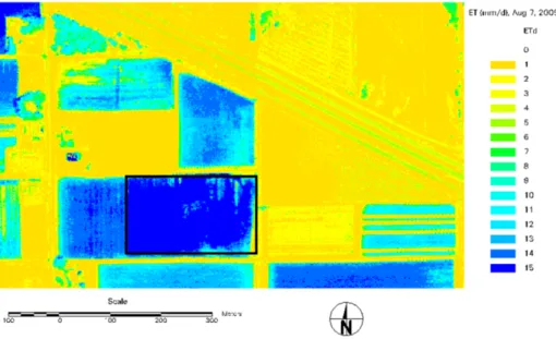
For DOY 187 the remote sensing SAT estimated alfalfa ET rate, at the lysimeter location, was 6.4 mm d-1 and for DOY 219 it practically doubled to 13.9 mm d-1. Figure 1 shows a map of ET for the surface conditions encountered on DOY 219.
On both days the LAI for the alfalfa was about 5.
The associated error in the estimation of the daily ET was -13.5% and +17.8% for DOY 187 and 219, respectively.
The larger over estimation error on DOY 219 mainly was due to the advective
conditions. Hot-dry (relative humidity of 29.7%) air at an average horizontal wind speed of 4.2 m s-1 increased the available energy for the ET process thus enhancing it about 44% above the alfalfa reference ET (ETr) value as computed using the ASCE-EWRI (2005) method. Under this climatological condition it appears that the SAT model did not account well for the extra heat integrated into the system (ET process). In contrast, METRIC depicted a smaller ET estimation error for similar climatological conditions; although resulting in larger errors for more heterogeneous, smaller biomass, and drier surfaces.
Figure 1. ET map for DOY 219 showing the lysimeter field (rectangle) in CO.
4. Conclusion
Two remote sensing based ET mapping methods (METRIC and SAT) were applied to high spatial resolution airborne multispectral remote sensing images acquired on semi-arid (advective) areas in Colorado and Texas. METRIC and SAT derived ET values were
contrast, the SAT method application resulted in a somewhat larger alfalfa ET estimation errors under similar conditions also which included advection.
Both methods resulted in reasonable accuracies although both have their limitations. METRIC on one hand relies on the ability and skills of the user in selecting the extreme hot and cold pixels in the remote sensing scene while SAT is a parameterized model which application is limited to the conditions in which it has been developed. Therefore, there is room for improving both methods and to define conditions under which one method would be more desirable over the other.
Acknowledgements. The financial support of the Ogallala Aquifer Program (USDA-ARS) and
that of CSU and the Colorado Agricultural Experiment Station is greatly appreciated. In addition, we are grateful for the collaboration, support and assistant received from the following individuals: Dr. Luis Garcia, Dr. Michael Bartolo, Dr. Christopher Neale, Dr. Allan Andales, Lane Simmons, Sale Straw, Dr. Tom Ley, Dr. Terry Howell, Dr. Prasanna Gowda, Karen Copeland and a number of technicians and student workers.
References
Allen, R. G., M. Tasumi, and R. Trezza. 2007a. Satellite-based energy balance for mapping
evapotranspiration with internalized calibration (METRIC)-model. ASCE J. of Irrig. and Drain. Eng., 133(4), 380-394.
Allen, R.G., M. Tasumi, A. Morse, R. Trezza, J.L. Wright, W. Bastiaanssen, W. Kramber, I. Lorite-Torres and C.W. Robison. 2007b. Satellite-based energy balance for mapping evapotranspiration with internalized calibration (METRIC)-Applications ASCE J. of Irrig. and Drain. Eng., 133(4), 395 - 406. ASCE-EWRI. 2005. The ASCE standardized reference evapotranspiration equation. Report by the American
Society of Civil Engineers (ASCE) Task Committee on Standardization of Reference
Evapotranspiration. Allen, R.G., I.A. Walter, R.L. Elliot, T.A. Howell, D. Itenfisu, M.E. Jensen, and R.L. Snyder (eds.), ASCE, 0-7844-0805-X, 204 pp., Reston, VA.
Bastiaanssen, W.G.M. 2000. SEBAL-based sensible and latent heat fluxes in the irrigated Gediz Basin, Turkey. J. of Hydrol., 229, 87-100.
Bastiaanssen, W. G. M., Menenti, M., Feddes, R. A., and Holtslang, A. A. 1998. A remote sensing surface energy balance algorithm for land (SEBAL): 1. Formulation. Journal of Hydrology, 212–213, 198-212. Bastiaanssen, W.G.M. 1995. Regionalization of surface flux densities and moisture indicators in composite
terrain: A remote sensing approach under clear skies in Mediterranean climates. Ph.D. Dissertation, CIP Data Koninklijke.
Brest, C.L., and S.N. Goward. 1987. Driving surface albedo measurements from narrow band satellite data. Int’l. J. of Remote Sens., 8, 351-367.
Brunsell, N.A., and R. Gillies. 2002. Incorporating surface emissivity into a thermal atmospheric correction. Photogramm. Eng. Remote Sens. J. 68, 1263-1269.
Brutsaert, W. 1975. On a derivable formula for long-wave radiation from clear skies. Water Resour. Res. 11, 742-744.
Chávez, J.L., T.A. Howell, D. Straw, P.H. Gowda, L.A. Garcia, S.R. Evett, T.W. Ley, L. Simmons, M. Bartolo, P. Colaizzi, and A.A. Andales. 2010. Surface aerodynamic temperature derived from wind/temperature profile measurements over Cotton and Alfalfa in a Semi-Arid Environment. In Proceedings of the American Society of Civil Engineers (ASCE), World Environmental & Water Resources Congress 2010 (EWRI).
Chávez, J.L., P.G. Gowda, and T.A. Howell. 2009. Modeling surface aerodynamic temperature in a semi-arid advective environment. In: Proceedings of the 2009 ASABE Annual International Meeting, Paper No. 096190, St. Joseph, MI: ASABE.
Chávez, J.L., Neale, C.M.U., Hipps, L.E., Prueger, J.H., and Kustas, W.P. 2005. Comparing aircraft-based remotely sensed energy balance fluxes with eddy covariance tower data using heat flux source area functions. Journal of Hydrometeorology, 6 (6), 923-940.
Elhaddad, A., and L.A. Garcia. 2008. Surface energy balance-based model to estimate evapotranspiration taking into account spatial variability in weather. J. of Irrig. and Drain. Eng., ASCE, 134(6), 681-689.
Foken, T. 2006. 50 Years of the Monin-Obukhov similarity theory. Boundary-Layer Meteorol. 119(3): 431-447.
Gowda, P.H., Chavez, J.L., Colaizzi, P. D., Evett, S. R., Howell, T. A., and Tolk, J. A. 2008. ET mapping for agricultural water management: present status and challenges. Irrigation Science, 26(3), 223-237. Gowda, P.H., J.L. Chávez, P.D. Colaizzi, S.R. Evett, T.A. Howell, and J.A. Tolk. 2007. Remote sensing
based energy balance algorithms for mapping ET: Current status and future challenges. Trans. ASABE 50(5): 1639-1644.
Menenti, M., and B.J. Choudhury. 1993. Parameterization of land surface evapotranspiration using a location dependent potential evapotranspiration and surface temperature range. In Proc. Exchange Processes at the Land Surface for a Range of Space and Time Scales. 561-568, Bolle HJ et al. (eds), IAHS Publ. 212. Monteith, J.L., and M. Unsworth. 1990. Principles of Environmental Physics. 2nd Edition, Edward Arnold
Press, 1990, New York, pg 291.
Neale, C.M.U., and B. Crowther. 1994. An airborne multispectral vide/radiometer remote sensing system: Development and calibration. Remote Sens. Envi. 49,187-194.
Su, Z. 2002. The surface energy balance system (SEBS) for estimation of turbulent heat fluxes. Hydrol. and Earth Syst. Sci. 6, 85-99.
Su, J., and L. Mahrt. 1995. Relationship of surface heat flux to microscale temperature variations: Applications to Boreas. Boundary-Layer Meteorol. 76, 291-301.
Wenbin, M., C. Zhongming, S. Linsheng, G. Wenliang, L. Xiuling, Y. Tingrong, P. Jan, H. Guanglun, and Y. Xiurong. 2004. A scheme for pixel-scale aerodynamic surface temperature over hilly land. Adv. Atmos. Sci. 21(1), 125-131.