Robot Goalkeeper: A robotic goalkeeper based on machine vision and motor control

(1)

FACULTY OF ENGINEERING AND SUSTAINABLE DEVELOPMENT

Department of Electronics, Mathematics and Natural Sciences

Taiyelolu Adeboye

September 2017

Degree project, Advanced level (Master degree, two years), 30 HE

Electronics

Master Programme in Electronics/Automation

Supervisor: Pär Johansson

Examiner: José Chilo (PhD)

Robot Goalkeeper

(2)

Preface

This report covers a thesis work carried out in partial fulfillment of the requirements of the master’s degree in electronics and automation at the University of Gävle. The thesis work was carried out at Worxsafe AB, Östersund between March and September 2017. The experience of carrying out the thesis has been quite interesting and instructive. While working on the thesis, I was also given the opportunity of taking up engineering responsibilities in cooperation with the staff of Worxsafe AB.

I would like to thank Pär Johansson and Bengt Jönsson, my supervisors at Worxsafe AB for their guidance, supervision and cooperation, and David Sunden, Magnus Lindberg and Patrik Holmbom of the mechanical department in Worxsafe, with whom I consulted and cooperated while carrying out the thesis assignment. I would also like to appreciate Julia Ahlen for her patience and tutorship in image processing, Professor Stefan Seipel for his tutorship and guidance in the image processing course and at the inception of this thesis and Asst. Prof. Niclas Björsell and Professor Gurvinder Virk for their tutorship in control. During my education in the university of Gävle, I have been under the tutelage of outstanding personalities to whom I am very grateful for the knowledge impacted and their patience and understanding. In no particular order, I would like to appreciate Dr. Jose Chilo, Dr. Daniel Rönnow, Mr. Zain Khan, Mahmoud Alizadeh. I would also like to thank Ass. Prof. Najeem Lawal, Mid Sweden University, for his tutorship and guidance in machine vision as well as Timothy Kolawole for his support during the thesis.

I have deep gratitude and respect reserved for Professor Edvard Nordlander and Ola Wiklund for their patience, understanding and special supportive roles they played in my education just prior to the thesis.

I owe a lot of gratitude to my family Temitope Ruth, Ire Peter, Ife Enoch for their understanding and support and my siblings, Ope, Adeyemi, Adeola and Kenny, who have always been supportive. I would like to also thank my parents-in-law, Victoria and Joseph Afolayan, for their support. Finally, I would like to appreciate my parents for their encouragement, support and faith in me.

Thank you.

Taiyelolu Adeboye

(3)

(4)

Abstract

This report shows a robust and efficient implementation of a speed-optimized algorithm for object recognition, 3D real world location and tracking in real time. It details a design that was focused on detecting and following objects in flight as applied to a football in motion. An overall goal of the design was to develop a system capable of recognizing an object and its present and near future location while also actuating a robotic arm in response to the motion of the ball in flight.

The implementation made use of image processing functions in C++, NVIDIA Jetson TX1, Sterolabs’ ZED stereoscopic camera setup in connection to an embedded system controller for the robot arm. The image processing was done with a textured background and the 3D location coordinates were applied to the correction of a Kalman filter model that was used for estimating and predicting the ball location.

A capture and processing speed of 59.4 frames per second was obtained with good accuracy in depth detection while the ball was well tracked in the tests carried out.

(5)

List of abbreviations

ARM: Advanced RISC Machine, is the name for a family of 32- and 64-bit RISC processor architecture.

eMMC: Embedded Multi Media Card, stands for a type of compact non-volatile memory device consisting of a flash memory and controller in integrated circuit.

USB: Universal Serial Bus.

RAM: Random Access Memory, a type of volatile memory.

DDR3: Double Data Rate type 3 RAM, is a type of synchronous dynamic RAM.

PRU: Programmable Real Time unit, is a subsystem of a processor that can be programmed to carry out functions in real time.

GPU: Graphics Processing Unit. PWM: Pulse Width Modulation

UART: Universal Asynchronous Reciever-Transmitter, a type communication of communication protocol.

SPI: Serial Peripheral Interface.

I2C: Inter-Integrated Circuit, a type of communication protocol. CAN: Controller Area Network

CSI: Camera Serial Interface, a type of high speed camera interface for cameras. GPIO: General Purpose Input Output

CUDA: Refers to a parallel computing and platform and API developed by NVIDIA. API: Application programming interface.

FOV: Field of VIEW

ROI: Region of interest, a region or part of an image frame that is of particular interest. V4L: Video for Linux, a driver for video on linux operating systems.

(6)

Table of figures

Figure 1 A high level visualization of the system ... 4

Figure 2 Image enhancement via histogram equalization ... 7

Figure 3 Demonstration of edge detection on an image ... 10

Figure 4 Differing perspectives of a chessboard as percieved by two cameras in a stereoscopic setup 11 Figure 5 Disparity in a stereoscopic camera setup ... 12

Figure 6 A sample environment model of the robot goalkeeper. ... 19

Figure 8 Chessboard corners identified during a step of camera calibration ... 23

Figure 9 Histogram equalization applied to the enhancement of an image ... 25

Figure 10 Histogram of RGB channels of the semi-dark scene before and after histogram equalization ... 25

Figure 11 Change of color space from RGB to YCrCb ... 26

Figure 12 Difference mask after background subtraction ... 27

Figure 13 Mask obtained after background subtraction, thresholding, erosion and dilation. ... 27

(10)

1 Introduction

The problem of object and depth detection and 3D location often comes up in several fields and is of vital importance in automated industrial systems, autonomous vehicle control and robotic navigation and mapping. Many different approaches have been employed in solving the problem with varying degrees of success in accuracy and speed. This thesis explores an approach that detects an object of interest in a 3D volume, determines its location and motion path, predicts its future pathway in real time at a very high frame rate. It also aims at determining appropriate actuation signal required for controlling a robotic arm in response to the detected object.

This thesis was initiated by Worxsafe AB in the process of creating a new product which is a robotic goalkeeper. The product required a robotic arm and a sensing system for detecting when shots are kicked, where the ball is, and predicting the flight path of the ball.

Since the system was meant to detect and act while the ball is still in flight, this created four problems which are:

1. Robust object detection.

2. Speed-optimized object location in 3D

3. Pathway prediction

4. Arm actuation and control.

In order to solve these four problems in real time, there is need for a process that is deterministic and fast enough to execute a minimum number of detection and location algorithms in order to achieve an accurate prediction which is followed by the actuation of the arm within a specific period of time. For this thesis, the time within which these four problems must have been solved, for each shot kicked, was set at 0.3 seconds.

Object detection has been well researched and is a problem that can appear simple in a controlled environment, especially one in which the image processing is not being done at the same pace as the image capture and where ambient illumination is controlled, steady and suitable. However, in a situation in which the object detection is to be done in an environment which is subject to some

(11)

change in ambient illumination and even extraneous sources of illumination the problem increases in complexity. The inclusion of the possibility of detecting very fast-moving objects real time further serves to require robustness in the detection algorithm.

Object location, in this work, was to be done with the aid of a stereoscopic camera setup only. The location was to be determined with the camera’s principal point as the reference frame. The location was to be determined in terms of depth, lateral and longitudinal offset from the principal point of the camera setup. In order to minimize the effect of noise in the processing and detection, a kalman filter was to be implemented and incorporated. Path prediction was to be done based on the detection and 3D location data obtained and actuation signals sent to the motor drive that controls the robotic arm.

There other approaches that could possibly explored in solving the problem addressed in this thesis. cameras could be combined with radar, multiple camera setup could be used, among other options. However, in this thesis, a simple stereoscopic camera was employed.

1.1 Background

The field of machine vision is an active focus of research and more interest is being generated with the advent of smart and autonomous automotive and industrial systems that are being strongly aided with LIDARs, cameras and image processing. Hence there have been significant research into topics that are related to the focus of this thesis work.

In their paper, Xu and Ellis[1] showed the application of background subtraction via adaptive frame differencing in foreground extraction, motion estimation and detection of moving objects. John Canny [2] developed the Canny edge detector among other computational approaches to edge detection while Bali and Singh[3] explored various edge detection techniques applied in image segmentation.

Black et al [4] showed the homography estimation in relation to a reference view while Yue at al[5] demonstrated robust determination of homography with the aid of a stereoscopic setup. Mittal and Davis[6] showed a method for homography determination with the use of multiple cameras located far from one another. Hartley and Zisseman in their book[7] explained the principles behind camera calibration, homography detection and reconstruction.

(12)

Kalman et al introduced the kalman filter in their publication[8] in 1960 while Zhang et al[9] and Birbach et al[10] demonstrated an application of the extended kalman filter to the problem estimation and prediction of the pathway of a ball in flight in robotics applications.

Zhengyou Zhang [11] developed a method for camera calibration, in a multi camera setup, using a minimum of two sets of synchronized images of planar objects with known structure without requiring foreknowledge of the object’s position and orientation.

1.2 Goals

The goals for the project are as follows:

❖ Evaluation of available embedded processors to determine the most suitable for the project. ❖ Evaluation of various camera systems and determination or construction of an appropriate camera

setup.

❖ Development of suitable algorithms for detection and 3D location ❖ Path prediction of the object of interest.

❖ Actuation of the robotic arm.

The overall aim of this project is the design of a system that runs autonomously once it has been setup and continuously detects and saves football shots kicked towards the goal. The system will consist of cameras for sensing, embedded system for processing the data obtained from the camera and an industrial drive for controlling the robotic arm.

(13)

The detection and object location were expected to be accurate and consistent with the actual real world location of the object being detected. The system should also be capable of functioning

satisfactorily in a well-lit environment with lightly textured background and should be adjustable such that interesting portions of the field of view of the camera and characteristics of the object to be detected can be varied.

1.3 Tools used in the project

The following tools were used in execution of the project:

1. Cameras

2. Image processing hardware

3. Embedded system to be used for sending control signals to the motor drive

4. Electric motor and gearbox

5. Controlled arm

(14)

6. MATLAB, Python, C++, OpenCV

7. Unix based OS/real time OS

1.4 Report outline

Chapter 1 of this report gives a basic introduction to the project, problem statement and motivation, overall aim, scope, tools, concrete goals and contributions involved in its execution. Chapter 2 briefly introduced relevant theory applied in the project. Chapter 3 explains the processes, measurements and results obtained in the project while chapter 4 discussed the results obtained. Applications,

implications and future work. Chapter 5 concluded the report and it was followed by references and appendices.

1.5 Contributions

The evaluation and selection of cameras and image processing platforms and design of image processing algorithm was done by the author of this report. Assistance in location setup, practical activities and measurements was provided by Timothy Kolawole by agreement with Worxsafe. The design, material selection and production of the mechanical arm was done by a team comprising of mechanical engineering staff of Worxsafe. The author also consulted Professor Stefan Seipel of the University of Gävle and Assistant professor Najeem Lawal of Mid Sweden University in the execution of the project.

OpenCV is a cross-platform, open-source library of functions for image processing and computer vision developed by Intel and Willow Garage. Python and C++ OpenCV interfaces were used in this thesis work.

CUDA is a platform and API developed by NVIDIA which provides functions for accessing and making use of the cores on NVIDIA GPUs for parallel processing.

Robotics, vision and control tool box for MATLAB was developed by Professor Peter Corke and some functions from the toolbox were used in generating 3D environment models for the project.

(15)

2 Theory

This chapter contains an overview of related theoretical terms and concepts that are relevant to

understanding this work. These are concepts were applied in the execution of the thesis work and were instrumental to obtaining the results.

2.1 Image processing methods

In this section image processing methods are briefly explained. The focus of this section are processing concepts which were principal to the functions and algorithms employed in this project.

2.1.1 Histogram equalization

Histogram equalization is an image enhancement method by which levels of intensities of pixels in an image can be adjusted in order to improve contrast. This method stretches the pixel values in an image to cover the available range offered by the image resolution. The formula is shown below:

𝑇(𝑘) = 𝑓𝑙𝑜𝑜𝑟((𝐿 − 1)𝑝

_𝑛

)

( 1)

Where pn represents the binned intensity level in the histogram and floor rounds the value down to the nearest integer value. T(k) above represents the pixel values of the transformed image and L represents the histogram bins. The formula can be simplified as shown below.

𝑁𝑒𝑤 𝑝𝑖𝑥𝑒𝑙 𝑣𝑎𝑙𝑢𝑒(𝑣) = 𝑟𝑜𝑢𝑛𝑑 ((𝐶𝐷𝐹(𝑣) − 𝐶𝐷𝐹𝑚𝑖𝑛) ∗

𝐿−1

(𝑀∗𝑁)−𝐶𝐷𝐹𝑚𝑖𝑛

)

( 2)

Where CDF(v) represents the cumulative distribution functions at the pixel position being recalculated and CDFmin represents the minimum CDF value. M and N represent the number of pixels along the height and width of the image.

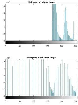
In this technique, the pixel value in each pixel position of the original image is used to calculate new values to be stored in each of the pixel locations in the new image referred to as the enhanced image. An example of an image enhanced via histogram equalization in the figure below. Histogram equalization enhances images and facilitates the identification of features in an image.

(16)

Figure 2 Image enhancement via histogram equalization

In the original image above, the outline of the the cloud, road, trees and other features were barely visible. The accompanying histogram shows that the pixel values were concentrated around a range between 170 and 240. In the transformed image which was enhanced via histogram equalization, the shape of the clouds, trees, roads, windows and other features were easily identifiable, and the image histogram showed a wide spread in pixel intensity.

2.1.2 Background subtraction

Background subtraction is a segmentation technique that is used for detecting changes and moving objects of interest in images. The seemingly static pixels in the image is referred to as the background while the new or moving object of interest forms part of what is known as the foreground. This technique is quite useful in identifying pixel portions of images in which there are changes that may signify the object that is to be detected in an image processing algorithm.

(17)

There are various approaches to extracting a foreground from a camera image and these approaches are normally complemented with morphological and thresholding operation to accommodate variations in image pixel values and to eliminate noise and unwanted artifacts from the image. Algorithms used in background subtraction include frame differencing, mean filtering, running gaussian average and gaussian mixture models.

The frame differencing method involves storing a copy of the background image and comparing it with subsequent images. The simplest form of comparison is done via arithmetic subtraction of the pixel values in the background image from the pixel values in the newly captured image being processed. The resultant image is referred to as a difference mask and it often consists of some unwanted artifacts along with the foreground if new objects or motion were introduced in the new image.

Difference mask[D(t)] = Current pixels[Im(t)] – Background pixels[Bgd(t)]

( 3)

The resultant difference mask is a grayscale image consisting of differences in the pixels values of the background image and the image being processed. After background subtraction, the unwanted artifacts are removed via thresholding.

The mean filter algorithm for background subtraction represents the image background at each time instant as the mean or median pixel values of several preceding images. The pixel values of this background are then subtracted from the pixel values of the image being processed. The resultant difference mask is also thresholded afterwards. This approach is also similar to the frame differencing approach.

The running gaussian average generates a probability density function (PDF) of a specific number of recently frames, representing each pixel by their mean and variance. The mean and variance is then updated with each new frame captured. Segmentation of foreground and background in each new frame is done by comparison of the pixel values in each new frame with the mean value of the corresponding pixel in the running gaussian PDF of the background.

𝑑 = |(𝑃

𝑡

− µ

𝑡

( 4)

𝜎

_𝑡2

= 𝜌 ∗ 𝑑

2

+ (1 − 𝜌) ∗ 𝜎

_𝑡−12

( 5)

(18)

Where d is the Euclidian distance, σ2_{is the variance in pixel value, µ is the mean of pixel values, P}

represents pixel values, ρ is the PDF temporal window and the subscript t indicates the progression of time.

The absolute value of the Euclidean distance between pixel value and the mean pixel value is divided by the standard deviation and compared with a constant value in order to segment the foreground from the background. Values greater than the constant identifies foreground pixels and background pixels otherwise. The constant is typically 2.5 but can be increased to accommodate more variation in background and decreased otherwise.

2.1.3 Thresholding

Thresholding is an image segmentation technique by which an image is segmented based on its pixel intensity values. The process usually involves comparing pixel values with a pre-specified threshold value below which pixel values are replaced with zero and above which the pixels are replaced with one. This output of this technique is normally a binary image.

Many techniques are employed to enhance the result of thresholding such as histogram shape and entropy-based methods, automatic thresholding, Otsu’s binarization method etc. The methods adapt the threshold value such that it varies with the image being processed facilitates the extraction of more useful information from the image frame. In this project, the thresholding was simple and

non-adaptive.

2.1.4 Edge detection

Edge detection is a method used for image segmentation by detecting pixel regions with intensity gradients or discontinuities which are representative of object boundaries. Common methods involve convolution of the image with a filter such as the Canny, Roberts, Sobel filters etc. It is a fundamental component of many algorithms in image processing. Convolution of an image with an edge detection filter results in an image consisting of lines representing object boundaries in the original image with all other information discarded.

(19)

Figure 3 Demonstration of edge detection on an image

2.2 3D reconstruction

In this section attention is given to concepts and methods that are related to image projection and 3D reconstruction. These concepts are essential to the extraction of depth information from camera images which are basically 2D pixel matrix representation of 3D scenes.

(20)

2.2.1 Stereoscopy

Stereoscopy is a technique, in image processing and machine vision, used for the perception or

detection of depth and three-dimensional structure using stereopsis. Stereopsis refers to the impression of depth perceivable in binocular vision as well as in multiple image capture devices capturing the same scene with some displacement between them. Stereopsis can also arise from parallax when a single image capture device is in motion while capturing a scene.

An object being observed by two cameras at the same time instant will result in some disparity in its location as observed by the two cameras. This disparity observed depends on the displacement between the cameras, their poses, parameters and the distance of the object being observed. If the displacement, poses and parameters are known, along with the disparity, then the distance of the object being observed can be calculated.

Figure 4 Differing perspectives of a chessboard as percieved by two cameras in a

stereoscopic setup

(21)

Images from two cameras with a displacement of 120 mm is shown in the figure above. In the scene captured by the two cameras, a man holding a chessboard is perceived differently by the two cameras. The two cameras have similar specifications and were synchronized to capture at approximately the same time instant. However, the chessboard seems to be angled differently and appears to the left in one image and to the right in the other. The distance of the chessboard, the man and other objects can be computed through the disparity in the pixel locations representing the objects of interest in the two camera views.

Figure 5 Disparity in a stereoscopic camera setup

A stereoscopic camera setup is shown in the figure above with the distance between the cameras represented by the baseline B, the left camera as the reference camera and the right camera offset from the left along x axis by a distance B and by a negligible distance along y axis. The ball being observed has image coordinates X0, Y0, Z0. The images are at distances fl and fr from the cameras respectively.

(22)

By similar triangles, 𝑋0 𝑍0

=

𝑥𝑙 𝑓𝑙

( 7)

Therefore

𝑥

_𝑙

=

𝑋0 𝑍0

∗ 𝑓

𝑙

( 8)

And

𝑦

_𝑙

=

𝑌0 𝑍0

∗ 𝑓

𝑙

( 9)

Similarly

𝑥

_𝑟

=

(𝐵 − 𝑋0) 𝑍0

∗ 𝑓

𝑟

( 10)

And ¨

𝑦

_𝑟

=

𝑌0 𝑍0

∗ 𝑓

𝑟

( 11)

The disparity in the ball position can then be used to calculate its distance from the left camera.

𝐷𝑖𝑠𝑝𝑎𝑟𝑖𝑡𝑦 𝑑 = 𝑥

_𝑙

− 𝑥

_𝑟

( 12)

𝑑 =

𝑋0

𝑍0

∗ 𝑓

𝑙

−

(𝐵 − 𝑋0)

𝑍0

∗ 𝑓

𝑟

( 13)

If both cameras are similar and having similar focal lengths,

𝑓

𝑙

= 𝑓

𝑟

= 𝑓

( 14)

And

𝑑 =

𝑋0 𝑍0

∗ 𝑓 −

(𝐵 − 𝑋0) 𝑍0

∗ 𝑓

( 15)

𝑑 =

𝐵 𝑍0

∗ 𝑓

𝑟

( 16)

Therefore

(23)

𝑍

0

=

𝐵

𝑑

∗ 𝑓

𝑟

( 17)

However, calculation of an object’s actual distance from a camera in real world units from 2D image data by triangulation requires some knowledge of the parameters of the cameras involved. The process of determining the 3D position of an object from 2D image data is known as image reconstruction. Calibration can be used to extract camera image projection parameters.

2.2.2 Image distortion

This refers to malformations in the image representation of a scene captured by a camera due to the deflection of light through its lenses and other imperfections in its design. Two of the most important factors that account for image distortion are tangential distortion and radial distortion. Radial

distortion results from the non-ideal deflection of light through the lenses of a camera, thereby resulting in curvatures around the edges of the image which are caused by variations in image magnification between the optical axis and the edges of the image. Tangential distortion results from the image sensor and the lens not being perfectly parallel.

Two common forms of radial distortion are barrel and pincushion distortion. Barrel distortion is observed in an image when magnification decreases toward the edges of the image, resulting in a barrel-like effect on the image. Pincushion distortion can be observed when image magnification increases towards the edge of the image and decreases vice versa.

Radial and tangential distortions are normally considered during calibration and the parameters describing these phenomena can be estimated during the process of calibration. Five parameters are commonly used to represent the forms of distortion. These parameters are collectively referred to as distortion coefficients. Below are simple formulae that can be used to correct for radial and tangential distortion. Radial:

𝑥

_{𝑐𝑜𝑟𝑟𝑒𝑐𝑡𝑒𝑑}

= 𝑥(1 + 𝑘

₁

𝑟

2

+ 𝑘

₂

𝑟

4

+ 𝑘

₃

𝑟

6

)

( 18)

𝑦

𝑐𝑜𝑟𝑟𝑒𝑐𝑡𝑒𝑑

= 𝑦(1 + 𝑘

1

𝑟

2

+ 𝑘

2

𝑟

4

+ 𝑘

3

𝑟

6

)

( 19)

Tangential:

𝑥

_{𝑐𝑜𝑟𝑟𝑒𝑐𝑡𝑒𝑑}

= 𝑥 + [2𝑝

₁

𝑥𝑦 + 𝑝

₂

(𝑟

2

_{+ 2𝑥}

2

_)]

_{( 20)}

(24)

𝑦

𝑐𝑜𝑟𝑟𝑒𝑐𝑡𝑒𝑑

= 𝑦 + [𝑝

1

(𝑟

2

+ 2𝑦

2

) + 2𝑝

2

𝑥𝑦]

( 21)

𝑟 = ((𝑥 − 𝑥

_𝑐

)

2

_{+ (𝑦 − 𝑦}

𝑐

)

2

)

1 2

_{( 22)}

Where

k1, k2 and k3 are coefficients of radial distortion, p1 and p2 are coefficients of tangential distortion and

x and y are pixels in a distorted image, xcorrected and ycorrected are pixels in an undistorted image and xc

and yc represent distortion center.

2.2.3 Image rectification

Image rectification is used, in image processing and machine vision, to project images taken by different cameras or by the same camera at different points in euclidean space onto a common image plane. It remaps the pixel points such that epipolar lines are aligned and parallel along the horizontal axis so that images taken by different cameras of a stereoscopic pair can be treated as representative of the same scene.

Image rectification in a stereoscopic setup basically makes use of projection parameters of the two cameras to compute the transformation matrices for each camera that can be used to align their image planes. Once the transform is determined, the images are transformed and both camera views can then be treated as depictions of the same scene.

2.3 Camera calibration

Camera calibration is the process by which the intrinsic and extrinsic parameters of a camera are estimated. These parameters are important in the application of stereoscopy for depth detection and object location in 3D. The parameters obtained from calibration are used to estimate a model that approximates the camera. Various approaches and algorithms are used for camera calibration; however, this report focuses on Zhang’s method which also the basis for the algorithm used in this project.

Zhang’s method of camera calibration makes use of images depicting a planar object or pattern with a known structure such, as a chessboard, in multiple views but no pre-knowledge of its orientation and position. Information about the object’s structure or pattern and several images of the object in various

(25)

orientations and positions are used by the algorithm in determining the image projection parameters of the cameras being calibrated.

Zhang’s method represents the relationship between a 3D real world point and its 2D representation as

𝑠𝕞 = 𝐴[𝑅 𝑡]𝕄

( 23)

Where

𝕞 = [𝑢, 𝑣, 1]

𝑇

_{( 24)}

represents the augment vector of pixel location of the point in 2D image.

𝕄 = [𝑋, 𝑌, 𝑍]

𝑇

( 25

)

represents the augment vector of object location in 3D space.

𝐴 = (

𝛼

𝛾

𝑢

0

0 𝛽

𝑣

₀

0

1 )

( 26)

represents the intrinsic matrix

α and β are the scale factors in image axes u and v (width and height) and γ represents the skew.

The extrinsic matrix is [R t] in the equation and represents the rotation and translation from world coordinates to camera coordinate.

The intrinsic parameters can be calculated thus

𝑣

₀

=

(𝐵12𝐵13−𝐵11𝐵23) 𝐵11𝐵22−𝐵122

( 27)

𝜆 = 𝐵

33

−

[𝐵132 +𝑣0(𝐵12𝐵13−𝐵11𝐵23)] 𝐵11

( 28)

𝛼 = (

𝜆 𝐵11

)

1 2

( 29)

𝛽 = (

𝜆𝐵11 𝐵11𝐵22−𝐵122

)

1 2

( 30)

(26)

𝛾 = −

𝐵12𝛼2𝛽 𝜆

( 31)

𝑢

₀

=

𝛾𝑣0 𝛽

−

𝐵13𝛼2 𝜆

( 32)

Where

𝑏 = [𝐵

₁₁

, 𝐵

₁₂

, 𝐵

₂₂

, 𝐵

₁₃

, 𝐵

₂₃

, 𝐵

₃₃

]

( 33)

𝕍𝑏 = 0

( 34)

and 𝕍 is a vector of estimated homography.

The method primarily involves capturing several images of the planar object with known structure or pattern in multiple camera views. A minimum number of two images is required by according to the proponent of the algorithm but a larger number, usually more than 10, has been found to give good results. The known feature points in the image are then detected and the data used for the estimation of intrinsic and extrinsic parameters. After estimation of the intrinsic and extrinsic parameters, the coefficients of radial distortion are estimated using least squares and then the parameters are refined using maximum likelihood estimation.

2.4 Kalman filter

Kalman filter is an iterative algorithm, based on linear quadratic estimation, by which noisy

measurements of dynamic systems can be accurately estimated and predicted. It involves an iterative process that builds a model of the system based on the observable parameters and generates, at each time-step, a prediction is made of both the observable measurements and the derivatives that cannot be measured directly. The prediction is then compared with the measured parameter and the model updated depending on the relative amount of belief reposed in the process versus the measurements. After the update, a new more accurate estimate is then generated for the system.

Estimates of the state and error covariance are predicted prior to acquiring measurement data using the formulae.

𝑥̂

_{𝑘|𝑘−1}

= 𝐹

_𝑘

𝑥̂

_{𝑘−1|𝑘−1}

+ 𝐵

_𝑘

𝑢

_𝑘

( 35)

(27)

Innovation residual, innovation covariance and Kalman gain are then calculated using values obtained from measurement. This is done after acquisition of measurement data and is part of the Kalman update.

ŷ

_𝑘

= 𝑧

_𝑘

− 𝐻

_𝑘

𝑥̂

_{𝑘|𝑘−1}

( 37)

𝑆

𝑘

= 𝑅

𝑘

+ 𝐻

𝑘

𝑃

𝑘|𝑘−1

𝐻

𝑘𝑇

( 38)

𝐾

_𝑘

= 𝑃

_{𝑘|𝑘−1}

+ 𝐾

_𝑘

𝑦̂

_𝑘

( 39)

A more precise estimate of the state, the estimation covariance and the measurement error are then made.

𝑥̂

𝑘|𝑘

= 𝑥̂

𝑘|𝑘−1

+ 𝐾

𝑘

𝑦̂

𝑘

( 40)

𝑃

𝑘|𝑘

= (𝐼 − 𝐾

𝑘

𝐻

𝑘

)𝑃

𝑘|𝑘−1

(𝐼 − 𝐾

𝑘

𝐻

𝑘

)

𝑇

+ 𝐾

𝑘

𝑅

𝑘

𝐾

𝑘𝑇

( 41)

𝑦̂

𝑘|𝑘

= 𝑧

𝑘

− 𝐻

𝑘

𝑥̂

𝑘|𝑘

( 42)

Where x̂k|k-1 is the state estimate at time instant k given measurements until k-1, x̂k|k-1 is the state

estimate at time instant k given measurements until k and x̂k-1|k-1 is the state estimate at time instant k-1

given measurements until k-1. At each time instant k, Fk is the state transition matrix, Bk is the matrix

of control input, uk is the control vector, zk is the observed state, Hk is the observation model, Kk is the

Kalman gain, Sk is the innovation covariance, Qk and Rk are the covariances of the process noise and

observation noise respectively. I in the equations represents a unit diagonal matrix and superscript T signifies a matrix or vector transpose. Pk|k-1 is the error covariance predicted at time instant k given

data up until time instant k-1, Pk|k is the covariance of estimation at time instant k given data up until

time instant k, Pk-1|k-1 is Pk|k is the covariance of estimation at time instant k-1 given data up until time

(28)

3 Process, measurements and results

The processes, measurements and results obtained in the thesis work are outlined and explained in this chapter with focus on those that are relevant to the goals of the project. Information is provided about the image capture and processor hardware, camera calibration and image processing algorithm, depth detection as well as results obtained.

3.1 Environment modelling

At the inception of the project, it was required that the robot environment be modelled in MATLAB. An environment was modelled in which the following were simulated and could be varied: robot location, goal post, camera location, elevation and tilt, ball kick zones, camera field of view and 3D volume monitored by camera. The MATLAB code for the model used functions from Robotics, vision and control toolbox by Prof. Peter Corke.

(29)

This model was used in evaluation of physical placement of hardware used in the project as well as in the process of selection of cameras. The model was also used to visualize zones with possibilities of occlusion and used for finetuning to reduce occlusion in pixel areas that can be of interest while the ball is in motion.

3.2 Evaluation and choice of cameras and processor

platforms

3.2.1 Processor platforms

It was required that the design be implemented on a processor platform that will be most suitable for speedy and real time on-chip image processing, low energy consumption and availability of peripheral interfaces for data transfer between cameras and the platform as well as other sensors and embedded hardware. The following processor platforms were provided by the company for evaluation:

1. Raspberry Pi 3 B+ 2. BeagleBone Black 3. Nvidia Jetson TX1

The specifications of the processor platforms are compared in table 3.1 below

Raspberry Pi 3 B+ BeagleBone Black Nvidia Jetson TX1 Processor on board Broadcom

BCM2837B0, ARM Cortex A53 64-bit

Texas Instruments Sitara AM335x, ARM Cortex A8 32-bit

ARM Cortex A57 64-bit

Processor speed 1.4 GHz 1 GHz 1.9 GHz

RAM 1 GB DDR2 512 MB DDR3 4 GB 64-bit DDR4

Non-volatile Storage Depended on MicroSD used

4GB 8-bit eMMC 16GB eMMC, SDIO and SATA

Graphics Processing Unit (GPU)

Broadcom VideoCore IV

PowerVR SGX530 NVIDIA Maxwell (256 CUDA cores)

(30)

Real Time Unit None 2 32-bit 200 MHz programmable RTUs

None

Power rating 5V, ~2.5A 5V, 210 – 460mA 5V, 3A Interfaces for

connecting cameras and image capture devices USB 2.0 CSI USB 2.0 PRU CSI (2 lane) USB 3.0 USB 2.0 Interfaces for other

peripherals

PWM, UART, SPI, I2C, GPIO

PWM, UART, SPI, I2C, CAN, GPIO

GPIO, I2C, SPI, UART

Table 1 Comparison of processor platforms

NVIDIA TX1 was selected among the processor platforms because it provides a possibility of faster image processing through parallel processing via its GPU cores which were accessed via OpenCV functions that are optimized for taking advantage of the cores via the CUDA library provided by NVIDIA. It was also observed that the TX1 has two high speed camera interfaces, CSI and USB 3.0, which can serve to reduce bottlenecks in the transmission of camera data.

3.2.2 Stereoscopy and image capture device

The choice of image capture device was determined by the processor platform and the fact that the depth detection to be implemented depends on stereoscopy. Stereolabs ZED camera was used in carrying out the thesis work because it consists of two image capture devices in a stereoscopic setup that can be accessed via a single USB 3.0 interface while remaining cheap in comparison with other products with comparable specification.

The stereoscopic camera provides synchronized frames from the two cameras as a single image which was easily accessible via the V4L driver in Linux OS. It was used at 720p resolution and 60 frames per second.

(31)

The specification of the camera is shown below:

Property Specification

Sensor size 1/3”

Sensor resolution 4M pixels per sensor, 2-micron pixels

Connection interface USB 3.0

Shutter type Rolling shutter

Lens field of view (FOV) 90o_{(horizontal), 60}o_(vertical)

Stereo baseline 120 mm (4.7 ”)

Configurable video modes 2.2K, 1080p, 720p, WVGA Configurable frame rates 15, 30, 60, 100

OS driver in Linux OS V4L (video for linux)

Table 2 Table of camera specification

3.3 Calibration of the camera

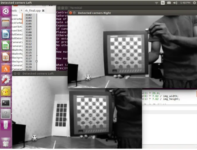
The stereoscopic camera was calibrated to extract its parameters and use it for depth detection. A chessboard was used for calibration and the calibration data was stored as yaml files on the non-volatile memory of the processor platform. These files were then accessed and the parameters used to process each captured frame in subsequent steps of the depth detection algorithm. The process of calibration used in this work was centered around an OpenCV function “calibrateCamera()” which itself is a derivative of Zhang’s method of calibration explained in section 2.6 of this report.

A chessboard was used for calibration since it is a planar object whose structure is known and easily specified. The number and dimension of squares on the board were first specified and stored in variables in the program. The board was then held in various positions about 20 times while the algorithm draws lines between the identified chessboard corners in the images from both cameras. The lines were then visually examined in order to ascertain that they properly aligned with the corners. when the lines were properly aligned the identified chessboard corners were accepted and discarded otherwise.

(32)

Figure 7 Chessboard corners identified during a step of camera calibration

When a pre-determined number of sets of identified corners were stored, the program calculates the camera matrix, the distortion coefficients, rotation vectors and translation vectors of the reference camera (left camera) from the set of identified chessboard corners and data about the dimension and number of squares on the chessboard. This is then followed by “stereoCalibrate()” which primarily tries to estimate the transformation between the reference camera and the other camera in a

stereoscopic setup. The rectification transform, projection matrices, disparity to depth map and output map matrices for x and y axis were then calculated for both cameras using “stereoRectify()” and “initUndistortRectifyMap()” functions in OpenCV.

The process used in this project can be summarized with the pseudocode below.

▪ Specify structure/pattern on the planar object to be used for calibration (object points) • Number of squares along height, no of squares along width, dimension of square box ▪ Specify number of images to be used for calibration

▪ While (number of images to be used is yet to be reached) • Capture image from left camera

(33)

• Capture image from right camera

• Enhance images by histogram equalization and smoothen to reduce noise • Convert RGB image to grayscale

• Find chess board corners using “findChessboardCorners()” function in OpenCV. • Draw the identified chessboard corners using “drawChessboardCorners()” function

in OpenCV.

• The images from both cameras with identified chessboard corners are displayed. • The images are visually inspected and accepted if correct or discarded otherwise. • The detected chessboard corners are stored in a vector

▪ Call calibrateCamera() function with the detected image corners and object corners as input argument and calculate camera matrix, distortion coeefficients, rotation vectors and translation vectors as output.

▪ Apply “stereoCalibrate()” function to estimate rotation and translation between the cameras as well as essential as fundamental matrix.

▪ Apply “stereoRectify()” to estimate the rectification transform and disparity to depth mapping matrix

▪ Apply “initUndistortRectifyMap()” for the estimation of the output maps.

▪ Write calibration data in a .yaml file so that they can be available when needed without a need to for calibration each time camera is used.

A snippet of code used for the calibration along with calibration parameters obtained for the camera used are available in the appendix A1 of this report.

3.4 Processing algorithm

Post-calibration processing was done in a continuous loop that starts with image capture and ends with depth detection and path prediction or determination of the absence of the object of interest within the field of view of the camera. The major steps involved in the algorithm are outlined in this section.

(34)

Figure 8 Histogram equalization applied to the enhancement of an image

The figure below shows histograms of pixel intensities in an image taken in a semi-dark room in figure 9 above. The histogram of pixel intensities before enhancement showed values that are

concentrated between 0 and 50 while a histogram of the enhanced image showed values that were well spread across the pixel intensity range.

The processing algorithm included an initial phase in which every frame captured was split into left and right images and remapped using the output maps obtained from calibration to remove distortion and reproject each camera view to depict the same scene. Each image was then smoothened and split into its constituent channels and each channel of the frames was enhanced by histogram equalization and merged into new frames that were then converted from RGB to the YCrCb color space.

Figure 9 Histogram of RGB channels of the semi-dark scene before and after histogram

equalization

(35)

Figure 10 Change of color space from RGB to YCrCb

The change in color space was made in order facilitate color-based image processing and reduce the impact of variation in illumination level on the subsequent image processing steps. The change in color space was done with the OpenCv function “cvtColor()” and setting the the color space conversion code to “COLOR_BGR2YCrCb”. A short snippet of code showing the initial pre-processing steps is included in appendix A4 of this report.

3.4.1 Foreground separation

Two approaches were initially explored for the background detection, the first approach continuously updated the model of the background after each frame while the second approach used a static pre-determined model of the background that was only updated after a long interval of time or at the cue of a pre-determined signal. The second approach was preferred above the first approach to reduce the amount of processing required while processing each frame in the loop.

A version of the mean filter algorithm was used to build a model of the background image. Several images up to a predefined number of images were captured and accumulated using the “accumulate()” function in OpenCV. Five consecutive images were used in this project. The accumulated images were then averaged and the resultant image was taken as a model of the background.

Background subtraction was applied to each frame after the initial processing steps of the algorithm. The foreground remains after subtracting the background, thereby identifying pixel areas that contain new data or motion and reducing the amount pixel area that needs to be processed by subsequent steps of the algorithm. The background subtraction was done by frame differencing of the pre-stored model of the background frame in YCrCb color space from the frames in YCrCb obtained in each step of the algorithm.

(36)

Figure 11 Difference mask after background subtraction

The difference mask obtained from background subtraction outlined the ball but included other unwanted image artifacts. Thresholding, erosion and dilation were then applied to the image to further enhance the result. A sample image of the end result of the morphological operations is shown below.

Figure 12 Mask obtained after background subtraction, thresholding, erosion and dilation.

3.4.2 Object and depth detection

The color and shape characteristics of the object of interest were primarily used in recognition of the object. These characteristics were stored at the beginning of the execution of the algorithm and the closest fit was used to determine the object of interest. The depth detection was done with pixel values around the center of gravity of the object of interest.

(37)

Image thresholding was done with a threshold value of 35 and an elliptical structural element of size 3 was used for erosion and dilation. While identifying contours using the “findcontours” function in OpenCV, RETR_EXTERNAL and CHAIN_APPROX_SIMPLE flags were set to ensure that only external contours were identified, and that the forms were simplified. The patterns in the pixel regions identified by the contours found were then treated individually and compared with a prestored model. Hough transform and processing of contours were applied on the foregrounds detected so as to determine pixel regions representing the ball and its location in the image.

(38)

The 3D location of the ball was calculated by triangulation of the pixel coordinates of the ball from both camera frames using the projection matrices obtained from calibration. The triangulation was done with the OpenCV function “triangulatePoints()” with the projection matrices and image points in both camera views as input parameters and object point in as the output parameter. The resultant object point vector was then normalized by dividing all the elements by the fourth element.

The object detection consisted of two parallel processes as shown in the flowchart above. The first consisted making use of Hough circles to detect the circular shaped blobs in the foreground of the L channel of the image and going through them to find the one with the best color and size match with the ball being detected. The second process employed the “findcontours()” function. It searched for all contours in the foreground of the Cr channel of the image and then, using the “minEnclosingCircle()” function, estimates the radius, area and image coordinates of its centre. These contours were also sorted based on best fit in terms of the color and size. At the end of processing for each frame, the results of both processes were compared and the best fit chosen.

• HoughCircles()

• For every circle detected o Obtain radius

o Build a ROI (region of interest) circumscribed in the circle o Compare the color in the ROI with the expected

o Choose best match

• FindContours()

• For each contour found

o Use minEnclosingCircle() to find radius, area and 2D location o Make a ROI on the contour

o Do comparison based on best color and size match. o Choose best match

Both processes can be summarized with the pseudocode steps above. The results obtained from both processes are taken into consideration in determining the ball location.

(39)

3.4.3 Speed-optimization

Some steps were taken to speed-up the image processing steps in each iteration of the algorithm loop. These steps explained briefly below.

1. Absence of object of interest in a camera view: Subsequent image processing were cancelled in processing a set of stereoscopic frames whenever the object of interest was not detected in one of the camera views. Since the processing steps involved a search for the ball in the image from the left camera, which is the reference, followed by a search in the image from the right camera, discarding subsequent processing steps whenever the ball was not detected in the left camera implies that no processing was done at all on the image from the right camera in each specific iteration step when there was no ball detected in the image from the left camera. This will result in significant savings of processor cycles.

2. Region of interest: Whenever an object of interest was detected within the field of view of one of the cameras, the possible location of the object in the field of view of the other camera was first estimated and a region of interest encompassing this region of interest was processed instead of the whole frame. This reduced the amount of processing required by a large margin. 3. Parallel Processing: The OpenCV functions used for processing image frames had CUDA

library support and were able to make use of parallel processing offered by the GPUs of the Jetson TX1 processor platform.

4. Localized depth detection: One of the core goals of this work is 3D location via depth detection in real time and at a high frame rate. A test of the API provided by the camera vendor yielded full frame depth detection at 11 frames per second which was below the requirement of the project. Therefore, localized depth detection was employed at the regions around the center of gravity of objects of interest. This resulted in significant gains in

processing speed. The resultant algorithm processed at a rate of 59 frames per second with the camera set to capture at 60 frames per second.

3.5 Kalman filtering and path prediction

Kalman filter was used in this thesis for filtering of the 3D location obtained and for predicting the future location of the object of interest. The filter was developed using the basic equations of motion and adapted to the flight of the object of interest. It was implemented using OpenCV functions.

The Kalman filter was designed with the X, Y and Z axial positions and velocities of the of the object of interest as its states for the state matrix. The time step, dt, for the filter was calculated from the time elapsed, in seconds, between each successive step of the image processing algorithm. The control

(40)

matrix included the effect of gravity on the motion of the object of interest along the Y-axis. The pseudocode below shows an outline of the application of the filter in the project. Further information about the filter is included in the appendix.

• Kalman filter was instantiated with its states by calling the OpenCV function

“KalmanFilter()”. This was done at the beginning of the program before continuous capture and processing.

• The transition, measurement, process noice covariance and measurement noise covariance matrices were initialized by direct access of the matrix elements or using the OpenCV “setIdentity()” function.

• During each iteration of the image processing and object detection process, the program estimates the time taken by calling the C++ “getTickCount()” function before and after the image processing in the iteration and finding the time elapsed based on the difference between the values obtained from the function calls. The time elapsed is set as dt, the time step, for the Kalman filter.

• At the beginning of each image processing and object detection iteration, the system checked if a ball has been detected in a previous iteration or if it was missed due to occlusion or false negative. If true, the “BALL_STATE” (a variable for indicating the state of the ball) was set to “IN_FLIGHT”.

• If the ball was found to be in flight

o A prediction of the ball location is made by calling the OpenCV function

“<KalmanFilter>.predict()”. <KalmanFilter> here refers to an object of KalmanFilter class.

o After the image processing and object detection was done in each iteration, the Kalman filter update was done by calling the OpenCV function

“<KalmanFilter>.correct()” and passing the measured positions of the ball to it as parameters. This updates the Kalman model filter with the measured data.

o If the ball was not detected while in flight, a prediction was made without correction and the prediction was taken as the location of the ball.

3.6 Actuation of the robotic arm

The 3D location of the object of interest was determined from the camera perspective but the robot arm to be actuated was located within the goal post area as seen in the environment simulation in section 3.1 of this report. Therefore, the detected position of the ball was calculated relative to the position of the pivot point of the robotic arm. This was done through a configuration step performed

(41)

prior to continuous image capture and processing and the detected location of the goalkeeper base was stored.

When a ball was detected and its 3D location calculated, the detected position of the ball from the camera viewpoint which had the left camera as its origin was translated to its relative displacement from location of the goalkeeper base using vector arithmetic.

𝑉

𝐺𝐵

= 𝑉

𝐶𝐵

− 𝑉

𝐶𝐺

( 43)

Where VGB represents the displacement of the ball from the goal keeper, VCB represents the

displacement of the ball from the camera and VCG represents the displacement of the goal keeper from

the camera.

The calculated displacement of the ball from the base of the goalkeeper was then communicated to the robot arm controller in order to actuate the arm. Three communication protocols were considered for this purpose: EtherCAT, UART and TCP. UART and TCP were implemented, tested and functional.

3.7 Results

3.7.1 Capture, processing and detection rates

NVIDIA’s Jetson TX1 was selected for the project and the setup was tested in a well-lit environment within the premises of Worxsafe AB. It had a processing rate of 59 frames per second with the camera set to capture at 60 frames per second. The detection was found to be robust and performed well in a moderately textured background. The testing was done with 500 captured and processed frames and an average of 59.4 frames was observed during the test.

3.7.2 Detection accuracy and limitations

It was observed that depth detection gave faulty values for depths less than 0.7 meter from the camera. This was also expected, as seen from the camera specifications. However, for ranges between 1 meter and 5 meters from the camera, the detection was accurate.

The system was tested in a poorly lit environment with plain colored balls. It was found to be functional but at a lower speed of about 41 frames per second.

(42)

(43)

4 Discussion

A core goal of the design was speedy and real time processing. The design was speedy and reasonably robust. It worked quite satisfactorily in well-lit test environment and at a lower frame rate in a poorly lit environment. The Kalman prediction also served to smoothen the results and predict location ball location during brief periods of occlusion.

Another approach that was considered in this implementation involves use of a sliding window that is activated after the first instance of detection of a ball or object of interest. This window would comprise of a region of interest that encompasses the previously detected location as well as all the possible locations of the ball. The window would then follow the pathway of the ball and only the content of the window would be processed. This will can also reduce the amount of processing required but there are possibilities that the window can be thrown out of sync with the actual ball motion when false positives are identified. This is not desired in the project.

The first weakness observed was that the operating system on the Jetson TX1 is a soft real time OS and as such does not have the deterministic behavior of a hard-real time OS. It was also considered that the camera seemed to create a bottleneck for the processing rate.

4.1 Applications

This approach for speeding up object and depth detection and actuation are widely applicable in industrial control systems especially in systems depending on machine vision such as pick-and-place machines. It can also be applied for recreation and entertainment purposes which are part of the essence of this project. In this instance, it will be developed further and used in the design of an automatic goalkeeper robot.

Speedy object and depth detection also find application in securing automated and autonomous

systems such in robot navigation and autonomous vehicle navigation. In this use case, it can be used in detecting oncoming objects and prevent collisions. It can also find applications in security systems especially in unmanned multi-camera setups.

4.2 Implications

Application speedy object and depth detection does not seem to have any known ethical or negative social implication. However, actuated systems that are developed to apply the concepts in automation

(44)

should be designed to be safe and extra care need to be taken to ensure that they do not hurt or damage property in use.

4.3 Future work

The system can be improved further to recognize and detect objects without first storing a model of the object to be detected. This can possibly be achieved with neural networks. A camera with a higher frame rate and resolution can possibly be used as well.

In this work, contours found in image foregrounds were treated sequentially. A better alternative could be to assign the treatment of these contours to parallel GPUs. This will reduce the amount of time spent processing the contours. Further simultaneous parallel processing of the synchronized frames which were obtained from the two cameras can also possibly increase the processing speed in situations where it is sure that an object of interest is within the field of view of the cameras.

A good number of applications and products include depth detection in which a depth map of the full frame captured is produced. This often results in a slower processing rate as every pixel in the frames are processed. An approach that can reduce the processing time and resource significantly would be to build a depth map of only the foreground pixels while pixel areas background can be updated with previously calculated values of the depths in the regions. It will be even better if these foregrounds are parallelly processed with the GPUs to reduce the time spent on them.

In this work, emphasis was placed on detecting a single object of interest. However, in many

applications, there can be several objects of interest in which case, these objects need to be identified along with their relative locations and then the appropriate line of action decided. This is analogous to the detection of several oncoming objects (or persons) by an autonomous robot or vehicle. It will need to be speedy in processing and understand the oncoming objects to mitigate accidents.

(45)

5 Conclusions

A speedy and efficient algorithm for object and 3D location detection was developed in this work. It combined image processing, stereoscopy and the enhanced functions and parallel processing

possibilities with the NVIDIA CUDA library and the Jetson TX1. An average frame rate of 59.4 frames per second was observed on a soft real time OS and it was fast enough for the robotic goalkeeper as specified by Worxsafe AB. The algorithm was also much faster than the full-frame depth mapping function in the API provided by the camera vendor.

The combination of processing hardware, camera and algorithm made it feasible to detect a ball in flight, track its location and motion with a stereoscopic camera and actuate a robotic arm to respond to the motion.

(46)

References

[1] M. Xu and T. Ellis. “TJ, Partial observation vs. blind tracking through occlusion”,

British Machine Vision Conference (BMVC 2002) pp. 777 -786, 2002.

[2] J. F. Canny. “A computational approach to edge detection”, IEEE Trans. on Pattern

Analysis and Machine Intelligence Volume: PAMI-8, issue 6, pp. 679 – 698, Nov.

1986.

[3] Bali, A., & S. N. Singh. “A Review on the Strategies and Techniques of Image Segmentation”, 2015 Fifth International Conference on Advanced Computing &

Communication Technologies pp. 113–120, Feb. 2015.

[4] J. Black, T.J. Ellis, and P. Rosin. “Multi view image surveillance and tracking”, Proc.

of IEEE Workshop on Motion and Video Computing 2002, pp. 169 – 174, Dec. 2002.

[5] Z. Yue, S. Zhou, and R. Chellappa. “Robust two camera visual tracking with homography”, Proc. Of the IEEE Int. Conf. on Acoustics, Speech, and Signal

Processing (ICASSP’04) 2004, volume 3, pp. 1-4, May 2004.

[6] A. Mittal and L. S. Davis, “M2tracker: A multi-view approach to segmenting and tracking people in a cluttered scene” Int. Journal of Computer Vision, pp. 189–203, 2003.

[7] R. Hartley and A. Zisseman, Multiple view geometry in computer vision, second edition, New York: Cambridge University Press, 2003, pages 239 - 260.

[8] R. E. Kalman, “A new approach to linear filtering and prediction problems”,

Transactions of ASME, Series D, Journal of Basic Engineering vol. 82, issue 1, pp. 35–

45, 1960.

[9] Y. Zhang et al, “Spin Observation and Trajectory Prediction of a Ping-Pong Ball”, 2014

IEEE international conference on Robotics and Automation (ICRA), pp. 4108 – 4114,

2014.

[10] O. Birbach et al, “Tracking of Ball Trajectories with a Free Moving Camera-Inertial Sensor”. In L. Iocchi et al, RoboCup 2008: Robot Soccer World Cup XII. RoboCup

(47)

[11] Z. Zhang, “A flexible new technique for camera calibration”, IEEE Transactions on

Pattern Analysis and Machine Intelligence, Vol. 22, Issue 11, pp. 1330 – 1334, Nov.

(48)

Appendix A

A1. MATLAB code for robot environment model

% This will be used to model the Robotic keeper's environment

% In order for this to work as it is, robotics and vision toolbox from % Peter Corke need to be installed and startup_rvc.m needs to have been run.

clear all; clc;

% Angle by which the camera is rotated/tilted

CB_rot = -pi/3.5; % Angle in radians equivalent to 180deg/3.5 = 51.4 degrees % Distances along the x, y & z axes by which the camera is translated

CB_Xtransl = 0; % Translation along the x axis CB_Ytransl = 0; % Translation along the y axis CB_Ztransl = 5; % Translation along the z axis

% Parameter for shifting forward the ball field in metres BF_Trans_X = 1;

BF_Trans_Y = 0; BF_Trans_Z = 0;

(49)

% Working distance - maximum distance of object, being tracked, from the % camera

WD = 10; % 10 metres

% No of vertical pixels of the camera Ver_Pxl = 480;

% No of horizontal pixels of the camera Hor_Pxl = 640;

% Ratio between the number of vertical pixels and number of horizontal % pixels of the camera

viewRatio = Ver_Pxl / Hor_Pxl;

% Angular field of view of the camera in the horizontal axis in degrees AFOV = 30;

% Horizontal AFOV in radians theta1 = AFOV * pi/180; % Vertical AFOV in radians theta2 = theta1 * viewRatio;

%%%% The camera box model

% Camera box points and their rotation and translations that determine the % camera displacement from original position

CB_P1 = [0.0 0.1 0.0]*roty(CB_rot) + [CB_Xtransl CB_Ytransl CB_Ztransl]; CB_P2 = [0.2 0.1 0.0]*roty(CB_rot) + [CB_Xtransl CB_Ytransl CB_Ztransl]; CB_P3 = [0.2 0.0 0.0]*roty(CB_rot) + [CB_Xtransl CB_Ytransl CB_Ztransl]; CB_P4 = [0.0 0.0 0.0]*roty(CB_rot) + [CB_Xtransl CB_Ytransl CB_Ztransl];

Robot Goalkeeper: A robotic goalkeeper based on machine vision and motor control

FACULTY OF ENGINEERING AND SUSTAINABLE DEVELOPMENT

Taiyelolu Adeboye

September 2017

Degree project, Advanced level (Master degree, two years), 30 HE

Electronics

Master Programme in Electronics/Automation

Supervisor: Pär Johansson

Examiner: José Chilo (PhD)