New Technology for Safe Critical Applications in Real Time

New technology for safe critical applications in real time

Bo Eliasson

Malmo University Technology and Society S-205 06 MALMO Sweden

Bengt J. Nilsson

Malmo University Technology and Society S-205 06 MALMO Sweden

Summary

Several techniques are available for constraint satisfaction problems. Most of them lack real time capability and distrib-uted computational properties. Configuration of complex sys-tems has today become a competitive edge, e.g. within e-busi-ness. The other side of the same coin can be used for diagnosis and simulation of safe critical applications. This paper gives a scientific background and comparison of methods for con-straint satisfaction problems implemented in real time environ-ment. Especially, the technique and its features of the array-based logic will be illustrated by three examples.

The examples are:

1. Modelling and simulation of system wide protection ap-plications of power systems

2. Modelling, simulation and implementation of safe critical switching in power systems

3. Modelling, simulation and implementation of safe critical systems of automatic train control

Array-based logic is a novel technology, which is founded on a geometrical representation of logic in terms of nested data ar-rays. In this representation, logical inferences are executed on finite domain systems by a few standardised array operations. In computational practice, array-based logic makes it possible

to solve large-scale constraint problems with

_M

combina-tions very efficiently. The major advantages of the technology are completeness, compactness, and speed of simulation (real-time capability), all of which derive from intrinsic properties of the underlying geometrical model. A system in array-based logic is considered analogously to electrical networks and is thus described by the constraints of the isolated elements as well as the constraints of the interconnected elements (the sys-tem topology). All syssys-tem constraints are eliminated in accord-ance with the methods known from electrical network theory and other engineering disciplines rooted in classical physics. The configuration space is represented explicitly in terms of nested data arrays and the system can therefore be simulated in real-time by co-ordinate indexing on these arrays. This data driven approach makes it suitable for parallel processing, which is an important quality for distributed systems. Keywords

Array-based logic, constraint elimination, configuration space, consistency verification,

system environment interaction, safe critical switching, real-time processing.

Introduction

In recent years, there has been an increasing interest in, what has variously been known as "constraint logic programming", "constraint satisfaction", or "constraint solving". This is due to the commercial interest in software tools for solving industrial problems characterised by a complex multitude of constraints or bindings, often related to some mix of purely technological considerations with those of competitiveness and efficiency. Typical in this respect is the configuration of complex products with a host of combinations, such as cars or computers. But constraint satisfaction problems also arise in many other areas as for instance production planning or job scheduling. In the computer industry, software tools for solving problems of this nature have been developed currently since mid 1980s. Origin-ally, these applications of constraint satisfaction were based on programming languages such as Prolog, that were developed in the field of AI (Artificial Intelligence) to cope with complex problems of a logical nature. Gradually, however, heuristic methods were introduced to solve such problems more effi-ciently. Today, as a result of this development, there are several commercial tools available on the market.

However, none of the commercial tools are suitable for real-time handling of large-scale systems with a multitude of con-straints like, say, railway interlocking systems or other systems to be discussed later. During 1993 to 1997 the two companies, Sydkraft AB and Bang & Olufsen Technology A/S, developed the new technological platform for solving complex constraint problems on finite domains. The work has been carried out in a joint EUREKA project (EU l007 'EMCON') in co-operation with the Electric Power Engineering Department at the Tech-nical University of Denmark, which has contributed with the scientific foundation of array-based logic. The basic idea of ar-ray-based logic is to explore the consequences of considering truth-values as physical measurements and to adopt the con-straint solving methods known from classical physics. Since 1997 the technology has further been developed and used in solving complex constraint problems. See the links:

www.arraytechnology.com and www.cybrant.com.

The Scientific Background

Although often presented as a new idea over the past decade, constraint satisfaction as a basic scientific concept dates back at least to the publication of Lagrange's Analytical Mechanics in 1788. In his famous work, Lagrange introduced the organ-ised handling of the constraints or bindings of discrete mechan-ical systems in terms of abstract geometrmechan-ical models, which since then has contributed the scientific foundation for dealing with discrete systems in physics and engineering. Thus, of per-tinent interest later on in this paper, Lagrange showed that if

the constraints could be eliminated, all possible states of the system could be described in terms of a set of independent parameters, the "degrees-of-freedom" of the system. Thus the equilibrium states could be determined by variational methods as a so-called "free variational problem". On the other hand, if the constraints could not be eliminated, he introduced the method of unknown multipliers to deal with them in non-elim-inated form. In the ensuing development over the following century or so, some of the most famous names in the history of physics introduced various classifications of constraints and devised methods for the organised handling of constraints fall-ing into these classifications. For example, as early as 1798 Fourier introduced inequality constraints in addition to those in terms of equalities, while in 1847 Kirchhoff introduced graph theory (in connection with his famous two laws) to deal with topological constraints in a systematic manner. Since the theor-etical concepts and methods for constraint satisfaction thus de-veloped in classical physics have stood the test of time for more than two centuries, it is puzzling to observe the complete lack of influence it has had upon the above mentioned develop-ment over the past decade in AI. In 1971, Cook showed that satisfiability, a special case of constraint satisfaction, belongs to the class of NP (non-polynomial)-complete problems. The year after Karp exhibited the intractability of NP-complete problems and proved seven more problems to lie in this class. These were applications from logic, scheduling, graph theory and set theory, in particular the well known travelling sales-man problem.

In the geometrical approach to logic introduced by Franksen [l], truth-values are considered as measurements with associ-ated scale-forms in the sense of physics rather than something intrinsic to language. The advantage of this view is that it now becomes possible to treat logical arguments as systems in terms of geometrical models, completely by analogy to physical sys-tems. The crucial point is that all possible solutions are con-sidered simultaneously without performing any assertion in or-der that elimination of the constraints can be performed prior to the act of assertion, which is then considered as an im-pressed force in mechanics. The set of all possible solutions may be formulated in terms of orthogonal arrangements of data, whence we talk about array-based logic. In a very ab-stract way we may consider these orthogonal arrangements as geometrical models spanned by a reference system of axes. This admits that these models may be associated with the no-tion of invariance under transformano-tions of reference frame. In other words, as Franksen pointed out in 1978 [l], the laws of propositional logic (as well as extensions to multi-valued lo-gic) may be considered by analogy to the laws of physics as those properties that remain invariant from under a mathemat-ical group of transformations. The importance of this view on logic ought not to not be underestimated, because it is now possible to show that predicate calculus and relational algebra are but isomorphic representations of the same abstract group as that characterising propositional logic. From a technological point of view, this is a tremendous simplification, since it means that reasoning can now be carried out in terms of only three, purely geometrical operations. Briefly described these operations are:

1. An outer product in the cartesian sense to establish arrays of all possible solutions;

2. The operation of taking out planes or hyper planes by equating two or more axes;

3. A reduction by logical addition or multiplication, which generalises the elimination process of the laws of the ex-cluded middle and contradiction to include the existential and universal quantifiers.

Although theoretically simple, this approach in terms of ortho-gonal arrays rapidly becomes unwieldy to implement on a computer. The aim of the technology of array-based logic is to preserve the mathematical foundation and simultaneously sup-port very large systems in industrial practice [4].

Systems in Array-based Logic

A system in array-based logic consists of a set of rules or rela-tions defining the constraints on an ordered set of state vari-ables. In accordance with classical logic, the relations are inter-preted as the premises of a logical argument.

The domain of a state variable is an ordered finite set (a list) with n unique items. The domain {False, True} of a proposi-tional variable is thus a special case with n=2. The list may be an explicit representation of all elements in a finite domain, or, in the case of large or maybe even infinite numerical domains, an ordered set of disjoint intervals.

The constraints of the entire system are determined as the con-junction of all relations. The complete state space of a system with N variables on domains with M elements may thus be

in-terpreted as an N-dimensional array with

_M

each of which can assume either of the truth-values false or not

(

₂

technological challenge is how to represent and manipulate large systems without the expected combinational blow-up in size.

To illustrate, let us consider a simple system on three Boolean variables A, B, C and a single relation or proposition

RO: (A or (not B))

⇒

The truth table of (l) consists of five legal and three non-legal combinations. Thus, the configuration space is not empty and the system is therefore consistent. In the case of large relations with a multitude of legal combinations, it is desirable to com-press the tuples into an isomorphic and more compact nested array form. The five legal combinations of (1) in the configura-tion space are:

RO: (2) A B C 0 0 0 0 1 0 0 1 1 1 0 0 1 1 0

This is carried out by the array operation compress:

Compress RO: (3)

A B C

0 1 0 1 0

0 1 1

The configuration space is now expressed in terms of two Cartesian arguments representing disjoint legal subspaces. The

Cartesian product of the first argument (0 1)(0 1)(0) yields four tuples, while the second argument 0 1 1 equals the remaining single tuple in (2). Although more isomorphic representations are possible, the great advantage of the above mentioned array form is that all logical inferences can be computed by just a few array operations on the tuples. For example, the state of each variable in the isolated system (l) is deduced simply by computing the unique items in the columns of (2) or (3):

SV: (4)

A B C

0 1 0 1 0 1

The list (4) is termed the state vector. We note that all four state variables are unbounded; that is, they may assume either of the truth-values O or 1 (the state of tautology). Thus, there are no constraints on the state variables when the system is isolated from the environment.

The state vector is the important means of interaction between system and environment. Let us assume that variable A is bounded to true due to external measurements:

SV1: (5)

A B C

1 0 1 0 1

The consequences are determined by joining the input state vector with the system relations (similar to a source on an elec-trical network or an impressed force in mechanics), and the resulting output state vector is deduced. The reader may verify by visual inspection of (2) that when A is bounded to true only two tuples of the configuration space are satisfied, and the new state vector SV2 is deduced with C bounded to false, while B is still a tautology:

SV2: (6)

A B C

1 0 1 0

In computational practice the state vector transformation (5)-(6) is very fast and even suitable for parallel processing. Note that in contradistinction to the usual IF -THEN rules of expert systems any assignment of variables can be used as input. For example, when C is bounded to true, we have the following output state vector:

SV2: (7)

A B C

0 1 1

The input state vector may also cause a contradiction. For ex-ample, this is the case on the relation (2) when A and C are both bounded to true. No tuples are satisfying this constraint. In general, the system constraints will be expressed in terms of more than just a single relation. For example, let us assume that the system (l) is extended with the relation R1:

RO: (A or (not B))

⇒

R1: C

⇔

We now have to eliminate the constraints of the individual re-lations as well as the connectivity constraints caused by the common variable C. In this simple example, it is possible to join the configuration space of the entire system (the

proposi-tion RO

∧

Join RO and R1: (9) A B C D 0 0 0 0 0 1 0 0 0 1 1 1 1 0 0 0 1 1 0 0

Equating the common C axes of the argument relations derives the result (9). This is one of the fundamental array operations termed colligation for making logical inferences [2]. The pro-cess of joining relations into singles is only possible on a small configuration space; in the case of large systems with a multi-tude of sparsely constrained relations the configuration space must be expressed in terms of the original relations but still with the connectivity constraints eliminated by colligation [4]. Generally speaking, the EMCON platform supports modelling, analysis, and simulation of large constraint satisfaction prob-lems on the technology of array-based logic sketched above. The major technological requirements are summarised as fol-lows:

l. Completeness: The complete state space with

_M

combina-tions must be addressable to ensure logical consistency of the entire system. Consistency is very important, especially when security is a critical factor.

2. Compactness: In order to cope with large systems in compu-tational practice, the internal data representation of a system model must be compact yet complete.

3. Real-time capability of simulation: The state vector trans-formation must be computed as fast as possible with predict-able processing time and allocation of memory.

The general form of this transformation is sketched in Figure 1.

=

Figure 1. System environment interaction

Illustrative examples of applications modeled by the array-based technology

Summary of example 1: A wide area protection system, at Sydkraft AB, was the first real-time application of array-based logic. The domain of the system was only 140 variables, all of which are Boolean. Nevertheless, the process of consistency

check followed by simulation directly on the consistent data model has proven its value and enhanced the ease of mainten-ance. Unfortunately the technique was not used in the imple-mentation phase of the project, due to lack of courage and knowledge at that time within the organisation. The decided approach to used conventional programming technique failed, due to test and maintenance problems, and the project was closed. The inherent complexity to handle loss of information, i.e. not defined states or signals due to disturbed communica-tion, in distributed real time systems makes it almost im-possible to use conventional programming methods. Summary of example 2: This example illustrates the array technology applied to power systems, a Ph.D. project sponsored by Sydkraft AB, for creation of complex coupling sequences in a secure and reliable way. The technology enables fast responses during simulation, due to the data driven ap-proach, instead of conventional program driven. The guiding rules for coupling sequences are divided into tactical, function-al (e.g. electricfunction-al) and operationfunction-al. The tacticfunction-al rules are mastered by the operator’s skill and therefore not included in the properties of the objects. The functional and operational properties, though, are included, and must be, in order to model safe critical systems. An example is Hemsjo; a medium sized substation in the Nordic power system, where the worst case of deduction takes 97 ms on a 400 MHz PC. The build phase of the substation takes 3.5 minutes and the database encloses 400 kb in compressed form, otherwise 900 kb. The number vari-ables are 1157 (including the interim varivari-ables), 586 relations and the free state space covers 2.2 10^304 combinations. Summary of example 3: By drawing a geometric representation (topology) of a railway station by using a conventional CAE tool, a list of objects (signals, connections etc) can be obtained. By associating each object with a set of predefined constraints, it is possible to automatically derive a list of all possible train routes. Each train route is represented by all the constraints or requirements for that particular train route. In other words, a schedule of all the possible train routes is automatically ob-tained, including all the requirements for a certain station. An example from a regular station, Borup, in Denmark: The rule base covers 237 kb (compressed), 1062 rules and 3000 vari-ables. The state space covers 2.1 10^78 combinations. The first two examples are further described below. The Wide Area P owe r Protection System

Svenska Kraftnät, Sydkraft AB and Vattenfall AB have jointly developed a wide area protection system against voltage col-lapse. [3]. The protection system uses measured analogue and digital values from several power stations and transformer sub-stations, while the logic deduction for coordinated actions in the transmission power system is based on binary created vari-ables. If a measured value or a combination of measured values exceeds a certain threshold, a relay operates. The binary signal may operate a switching device either locally or in a remote station. The logical decision-making process is implemented in the Sydkraft SCADA system. The system wide protection is implemented in three (local control rooms) out of four (central control room) computer system nodes. Specific actions are then ordered from the SCADA system, such as switching of shunt reactors and shunt capacitors, start of gas turbines, request for emergency power from neighbouring areas, disconnection of low priority load and, finally, load shedding. Shedding of high priority load also requires a local low voltage criterion in order

to increase security. The Swedish transmission system is char-acterised by a large amount of power transmitted from the hy-dro power stations in the North to the load centres in the South. In December 1994 the Baltic Cable 600 MW HVDC link was commissioned from the very South of Sweden to Germany. To be able to use the full export capacity another 600 MW have to be transmitted through the South of Sweden. On the other hand the HVDC link can provide emergency power equal to the dif-ference between the actual point of operation up to 600 MW import (so far the capacity of the cable is limited to 250 Mw caused by limitations on the German AC side). The maximum change of power will probably be limited to 600 MW

(presently the limit is 150 MW). Based on the requirements for power transfer through the Baltic Link, the new possibilities provided by using the link for power and the experiences from the temporary voltage controlled load shedding system, it was

SCADA SYSTEM RTU < U _SEE3 X CONNECTED1 TO THE GRID T4 LOGICAL EQUIPMENT CICUIT BREAKER FOR DISCONNCTION OF X SEE1 T = . S4 1 0 U = 3 380 kV Q BVT = 200 Mvar SPECIAL PROTECTION SYSTEM IN OPERATION X VOLTAGE 1 CONTROL IN OPERATION X NOT DISCON-1 NECTED THE LAST

MINUTES 5 < U _AVA3 < U _SÅN3 < U _HEÖ3 < U _BED3 < U _NBO3 > Q_BVT_G1 > Q_BVT_G2 > Q_SVP G2 > Q_SVP G1 BVT_G & G OUT1 2 t3 t2 t1 X _SB1 CB > = 4 > = 1 > = 1 & a b c d

Figure 2. Special protection system for disconnection of a 440 kV shunt reactor of 150 Mvar.

decided to design a wide area protection system against voltage collapse. The basic power system ideas behind the chosen signals and threshold for creation of the binary signals schemes are given in [3]. The only data used for this special protection system, transmitted in the SCADA system, are the input signals, which are available in all the system nodes. In each node the logic, for actions to be performed in substations controlled by that node, are in continuous operation. The result of the design procedure was a set of logical schemes for each node to control the devices and perform the objectives. One scheme is shown in fig. 2 and will serve as an illustration in this paper. The logical constraints of the protection system in fig. 2 can be expressed solely in terms of binary variables. Table A below defines the logical constraints on the system, while Table B explains the domain of some binary state vari-ables. Further information is given in [5]. In order to verify and simulate the system, the symbolic form of the relations are compiled into the standard array form sketched in the previous section. The topology of the logical network in fig. 2 is a simple structure with one output variable Xl-SE derived from a given set of input variables. Thus, in this isolated case with just a few variables the consistency of the system is quite obvious and may be verified by visual inspection. In general, a manual check is not satisfactory. A major advantage of the technology of array-based logic is the capability of automatic consistency verification of the entire system with many interconnected sub-systems (distributed sub-systems).

Table A. System constraints applied to fig. 2.

R0 t1=Q_BVT_G1 + Q_BVT_G2 + (BVT_G1 and BVT_G2) >= 1

R1 t2=Q_SVP_G1 + Q_SVP_G2 >= 1

R2 t3=U3_SEE + U3_BED + U3_NBO + U3_AVA

+ U3_SAN + U3_HEO + t1 + t2 >= 4

R3 X1_SB = (a and b and c and not d and t3)

The statements, R0 to R4, constitute the program code need to be written in order to describe the functionality of the scheme in fig.2.

Table B. Domain of binary state variables of fig. 2.

# Variable Explanation Domain

0 U3_SEE Voltage level in Sege 0: Normal

1: Low

1 U3_BED Voltage level in

Breared 0: Normal1: Low

….. ….. ….. …..

16 X1_SB Trip signal to circuit

breaker X1 SEE in Sege

0: Off 1: On

The first step in the modelling process is to establish the stand-ard array form of each isolated relation in Table A. The second step is to eliminate the connectivity constraints defined by the common variables of the relations. This is carried out by col-ligation, and the result is a complete array form representing the configuration space.

When the complete array form has been established, we are ready to perform the state vector transformation on the system. Obviously, traditional programming techniques or even in hardware could deduce the output state X l-SE very efficiently. Why is the array implementation then a better choice as far as e run-time environment is concerned? Firstly, maintenance of the system due to modifications in the system constraints is very easy, when all logic control structures are data rather than something intrinsic to programs. Secondly, the array represent-ation makes it possible to deduce results in either direction, for example the possible inputs implying a given output. Thirdly, the state vector introduced in the previous section includes the states of contradiction and tautology (don't care) as special states of the variables. This is important in the case of missing input signals. For example, if variable b in fig. 2 is unknown due to communication faults, the deduced output X 1 SE is also a tautology. Fourthly, the expert can do the programming and simulation according to Table A and the software and real time system experts only embed the application in the SCADA sys-tem. No non-application expert is messing up the content of the Array Database, ADB, which is very important when develop-ing safe critical applications.

The rest of schemes and variables included in the protection system are treated in the same way.

Safe Critical Switching in Power System

The second example illustrates the array technology applied to power systems for creation of complex coupling sequences in a secure and reliable way.

The technology enables fast responses during simulation, due to the data driven approach, instead of conventional program driven. The guiding rules for coupling sequences are divided

into tactical, functional (electrical) and operational. The tactic-al rules are mastered by the operator’s skill and therefore not included in the properties of the objects. The functional and op-erational properties, though, are included, and must be, in order to model safe critical systems.

The intention is to make an array theoretic as well as a graph-ical definition of the objects, the primitive properties, in power system network.

After the definition of the primitive properties of the objects, it should be possible to model a part, e.g. a substation or an area, of the network to test the legality and consequences of coup-ling sequences in that specific area.

Topology and variable representation

Graphs are often a very efficient way to model a system con-taining topological information. Some graph models can be close to the system i.e. the topology of the graphs can easily be identified in the physical system. In others, the topological data can be more or less hidden in the system.

For systems like power and railway systems, at least one set of topologic information is obvious. The system itself is a net-work of topological information. The diagram of an electric network is an example of a model with topological data that can be found directly in the physical system. The topology of an electric diagram is isomorphic to the physical system. The Roth diagram of electrical systems is an example of a model that is not isomorphic to the physical system. This dia-gram constitutes the formulation and solution of the electric network problem. Since the topology of Roth diagram is based on Ohm’s and Kirchhoff’s laws of resistive electric networks the topology of Roth diagram is not isomorphic to the physical system.

In order to handle safe critical applications in an electrical net-work, the definition of a minimum set of variables and graph representation is crucial. In [6] it is shown that an optimal rep-resentation is to use both voltage and current as compound variables.

When connecting two electric elements it is equivalent to make two colligations: voltage and current. Often it does not make sense to connect two voltage variables without also connecting two current variables. If this should be reflected graphically, an electric stub, “p” should be added representing both a voltage and a current. Using a nested type of variables, containing both voltage and current, achieve this. This nested representation of variables is supported by the array database in the form of “compound identifiers”. The new definition and extended col-ligation graph is shown in fig. 3. Now the graph and the elec-tric diagram are isomorphic, and this makes it easier to model the electric network. See also [7].

Graphical definition Extended colligation graph Relation types Variable types

p1 p2 p2 p1 p2 p1 p : u, i Boolean, Boolean k l K L P0 P1 P2

Definition of the electrical objects

All the objects included in a general coupling sequence have to be modeled according to its specific set of rules. In order to achieve this, a proper choice of the domain of the variables, as-sociated to each object, have to be defined.

Two different and conflicting guidelines are important when deciding a proper domain of a specific variable.

1) The larger the domain, the more accurately the physical variable is described.

2) The smaller the domain, the smaller the resulting array data-base and bigger systems can be built.

This means that the domain of a variable must be large enough to describe the physical quality of the variable in an adequate way, but no more.

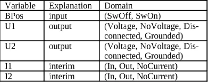
The states of a circuit breaker can be described by five vari-ables. Two of type, “Voltage”, describing the voltage of the two terminal points. Two of type, “Current”, describing the current flow in the two terminal points, and one of a binary type, that describe whether the breaker is open or not, see Table C. Following variable definition is used in the case of breakers. The two current variables are marked as interim be-cause these variables will be eliminated in order to reduce the database, but needed during the modelling phase or description of safe critical properties of the breaker.

Table C. Circuit breaker variables and domain.

Variable Explanation Domain

BPos input (SwOff, SwOn)

U1 output (Voltage, NoVoltage,

Dis-connected, Grounded)

U2 output (Voltage, NoVoltage,

Dis-connected, Grounded)

I1 interim (In, Out, NoCurrent)

I2 interim (In, Out, NoCurrent)

These domains give a state space of 288 possible combinations. The major part of the logical definition consists in dividing the possible combinations into legal and illegal combinations. By inspecting the rules regarding the breaker defines the legal combinations. Both electrical and coupling rules must be ex-amined.

Electrical rules of a breaker

1. No current can flow through an open breaker. 2. No current can flow if not both voltage variables are

Voltage.

3. If the current at one terminal is “In”, the current at the oth-er must be “Out”.

4. If no current is flowing at one terminal, no current can flow at the other terminal.

5. If the breaker is closed, there cannot be voltage at one ter-minal and no voltage, disconnected, or grounded at the other terminal.

Coupling rules of a breaker

The breaker cannot be used as disconnector, i.e. if there is voltage or no voltage at one terminal the other terminal cannot be disconnected or grounded even if the breaker is open. Legal combinations of a breaker

After the rules have been examined and the illegal combina-tions are found, the combinacombina-tions in Table 1 remain as legal. These combinations can be verified that they not violate any of the rules. The number of legal combinations turns out to be 16 and constitutes the primitive description of a circuit breaker. This table can now be written to a text file and made accessible to the build tool of the array database software.

Disconnector

The disconnector symbol is shown in fig. 4. The conditions for a disconnection is a visual gab between the two terminals and that the disconnection is locked. The disconnector can fulfil both these demands. However, it cannot be used to break cur-rent under normal circumstances.

pos i1 u1 i2 u2

SWON IN VOLTAGE OUT VOLTAGE SWON OUT VOLTAGE IN VOLTAGE SWON NOCURRENT VOLTAGE NOCURRENT VOLTAGE SWON NOCURRENT NOVOLTAGE NOCURRENT NOVOLTAGE SWON NOCURRENT DISCONNECTED NOCURRENT DISCONNECTED SWON NOCURRENT DISCONNECTED NOCURRENT GROUND SWON NOCURRENT GROUND NOCURRENT DISCONNECTED SWON NOCURRENT GROUND NOCURRENT GROUND SWOFF NOCURRENT VOLTAGE NOCURRENT VOLTAGE SWOFF NOCURRENT VOLTAGE NOCURRENT NOVOLTAGE SWOFF NOCURRENT NOVOLTAGE NOCURRENT VOLTAGE SWOFF NOCURRENT NOVOLTAGE NOCURRENT NOVOLTAGE SWOFF NOCURRENT DISCONNECTED NOCURRENT DISCONNECTED SWOFF NOCURRENT DISCONNECTED NOCURRENT GROUND SWOFF NOCURRENT GROUND NOCURRENT DISCONNECTED SWOFF NOCURRENT GROUND NOCURRENT GROUND

Table 1: Legal Combinations for a circuit breaker

Logical definition of a disconnector

The rule regarding the breaking of current says that if a load current is flowing, the next position of the disconnector must not be disconnected. This means that the next position of a dis-connector must be represented by a variable. Table D shows the variables and the domains.

The next position variable makes the disconnector a dynamic primitive according to chapter 10.4, [6]. Of cause, the current position of the disconnector must also be represented. The two position variables form a dynamic variable. Apart from the two position variables, two sets of voltage and current variables are needed. This variable definition gives a state space of 2304 possible combinations.

Disconnected Connected

Disconnected and locked

Connected and locked Figure 4. Disconnector symbols

Table D. Disconnector variables and domain.

Variable Explanation Domain

NextPos output (SwOff, SwOn,

SwOff-Lock, SwOnLock)

Pos input (SwOff, SwOn,

SwOff-Lock, SwOnLock)

U1 output (Voltage, NoVoltage,

Dis-connected, Grounded)

U2 output (Voltage, NoVoltage,

Dis-connected, Grounded)

I1 interim (In, Out, NoCurrent)

I2 interim (In, Out, NoCurrent)

Electrical rules of the disconnector

1. No current can flow though a disconnected disconnector. 2. No current can flow if the voltage variables are not

Voltage.

3. If the current in one terminal is In, the current in the other must be Out.

4. If no current is flowing in one terminal, no current can flow in the other.

5. If the disconnector is connected, there cannot be Voltage at one terminal and NoVoltage, Disconnected, or Ground at the other.

Coupling rules of the disconnector

1. The disconnector cannot be used to break load current or charging current when connected to a long, remote open end, line. If a load current is flowing, the next position cannot be disconnected.

2. The disconnector must be unlocked before it is operated. If the current position is “disconnected and locked”, the next position must remain “disconnected and locked” or changed to “disconnected”. This is also the case for “con-nected and locked”.

3. It is not legal to ground through a disconnector if it is not connected and locked.

4. An area cannot be considered disconnected before the dis-connector is locked.

Special situations

In some rare situations, it is legal to break current using a dis-connector. This may only be done if a parallel connection ex-ists, i.e. commutation of current.

After the rules have been inspected, 90 legal states of the dis-connector remain.

The same procedure is repeated for all the objects (trans-formers, ground connectors etc) in order to define the legal combinations needed for modeling.

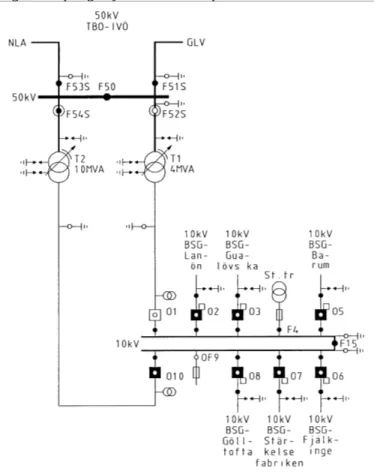
Modeling of power system

After the definition of the primitives a regular substation can be modeled. Normally one or more stations are involved in a coupling sequence. In the following, the station Bäckaskog will be modeled. The normal coupling diagram of Bäckaskog, a CAD-drawing from Sydkraft AB, is shown in fig.5. During the simulation and the building phase of the substations a soft-ware package named, G2, was used. Gensym Inc., USA, devel-ops the G2- software. G2 is an object-oriented expert system with real time capability and off-line simulation. In order to build a general part of a power system a special library includ-ing all couplinclud-ing objects was developed.

Figure 5. Bäckaskog. Normal coupling conditions

All the coupling sequences start normally from a predefined state.

The normal coupling situation is automatically loaded when G2 is started and the workspace of the station is shown. To define the normal coupling topology in G2, the model is changed until it is identical to the normal coupling situation. Then the “Save as Normal Coupling” - button is pressed. Figure 6 shows of the normal coupling of Bäckaskog in a workspace of G2. The T2 transformer supplies both the 10 kV busbars, while the T1 transformer is idle.

An example of a coupling sequence;

Figure 6: G2 generated normal coupling of Bäckaskog The goal of this coupling sequence is to prepare the cable between the transformer T2 and the breaker, O10, for mainten-ance. After the work is done the coupling sequence, must bring the station back to normal coupling.

Obviously, the supply of the 10 kV busbars must be moved to T1 while the maintenance work is going on. In addition, the cable must be grounded before the area can be released for maintenance.

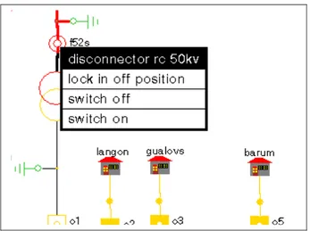
The first step is to connect T1. The primary side of the trans-former must be connected first. Connecting the

Figure 6

disconnector F52S does this. At the G2 model the “switch on” menu point at the pop-up menu is selected. The pop-up menu, shown in fig. 7, appears when the discon-nector is selected. The array database is automatically consul-ted to check if the coupling is legal. If it is, the consequences of the coupling are retrieved from the array database and are directly shown at the model. The levels of the 50 kV cable to the transformer and 10 kV cable from the transformer are changed to “VOLTAGE” and changing the color of the two cables shows it. Now the transformer must be connected to the busbars.

Closing breaker, O1, achieves this. After the coupling, the 10 kV busbars are supplied from both the transformers.

It is now possible to break the supply from the T2 transformer without affecting the power supply to any customer. The breaker O10 is opened in order to achieve this.

Figure 7. Pop-up Menu

The disconnectors F54S and F10S can then be disconnected in order to isolate the area. The color of the cable is changed to black, which shows that no voltage is applied to the cable. Now the user commits an error that violates the rules of coup-ling. Having isolated T2 and the cable connections to it, the op-erator believes that it is legal to close the ground connector between T2 and O10. Electrically this operation causes no problem because the area is without voltage. However, the op-eration violates one of the security rules. It is not legal to ground an area before it is isolated and locked in this state. The problem is that none of the two disconnectors is locked. Hav-ing neglected the detail about lockHav-ing the disconnector, the op-erator tries to connect the ground connector.

The array database is consulted to ensure that the operation is legal. The answer from the array database is an error code and a text explaining that the operation causes a contradiction. The user is notified and the operation is ignored.

F54S and F10S are then locked in the disconnected state in or-der to fulfil the rules. The G2 model is updated by changing the icons of the two disconnectors. The color of the cables is also changed. It is now cyan to show the operator that the area now is isolated and locked. Now it is legal to connect the ground connector.

The color of the cable between the transformer T2 and the breaker O10 is changed to green. This tells the operator that the cable is now grounded, and the maintenance work can be-gin.

The little piece of cable between O10 and the locked discon-nector is still cyan. This indicates that this site of the breaker cannot be considered grounded. Even if the breaker were closed, the cable would remain cyan, because it is not legal to ground through a breaker. The same thing can be observed with the cable between T2 and F54S.

The last item in this part of the coupling sequence is to send work permission regarding the 10 kV cable between T2 and O10 at BSG. The couplings must not continue before operation permission is received from the maintenance worker at BSG. When the maintenance work is finished and the operation per-mission is received, the couplings can continue in order to bring the station back to normal coupling. These couplings are not shown here.

For further information see [6]. Conclusion

The wide area protection system is the first real-time applica-tion of array-based logic. The domain of the current system is

just 140 variables, all of which are Boolean. Nevertheless, the process of consistency check followed by simulation directly on the consistent data model has proven its value and enhanced the ease of maintenance.

The extended colligation graph contains all the information needed to build an array database. The relations are defined as ties binding the variables together. The nodes in the extended colligation graph represent the system variables. Different types of ties can be defined in a way that makes it easy for the user to identify the primitive type it represents. This is called the graphical definition. The logical definition of a primitive holds the restriction of the variable combinations. It can e.g. be given in form of a logical table. The primitives should be small. When they are defined, it must be possible to go through every variable combination to determine if it is legal or not. Afterwards different primitives can be combined into new primitives.

Of cause, it is necessary to have some knowledge of array-based logic in the primitive definition phase. The primitives are simply combined in their graphical form and the input to the array database is automatically generated with no risk of errors. This modeling method is best used on systems with some build-in topological information e.g. electric networks or railway system. In addition, the primitives should be defined in a way that makes the diagram of the system and the extended colligation graph isomorphic. If they can be made isomorphic, drawing a diagram of the network using the defined primitives and a graphical platform like e.g. G2 does the modeling of an electrical network.

When the graphical and the logical definition of the primitives are finished, connecting the primitives according to the physic-al system generates the array database. A person without knowledge of array-based logic can do this process. To make the modeling phase easy, a graphical building tool must sup-port it. In this project, G2 from Gensym Inc. is used as graphic-al tool both during the modeling phase and later during the simulation. G2 offers the opportunity to build the model by making instances of the defined primitive. The primitives are then placed on a workspace and connected to reflect the phys-ical system. The input text file is automatphys-ically generated by G2. Afterwards the build tool within the array database is auto-matically called by G2 and a binary array database is built. The operator is of cause warned if any problems occur during the building of the binary array database, or if it turns out that the database is inconsistent.

Using the array database can do several different types of sim-ulations and checks. The most fundamental is the consistency check, which is performed during the building of the binary ar-ray database. The check ensures that the model has at least one legal variable combination. Normally an array database model has several legal variable combinations, but configuration problems with only one legal solution exist. In these, the task would be to identify the legal combination. Even though the model has more legal combinations, some of the variables could be bound to specific values. These values can be identi-fied by the array database and shown in the G2 model.

Another type of simulation is the validation of a model. In this, some of the variables are bound and a deduction can be made on the remaining variables. It is thereby possible to validate that the model is working as expected. Since no distinction is made between input and output variables in this simulation, it is possible to bind variables that are normally considered

out-put to deduct the inout-put that would generate this outout-put. This type of simulation is shown in the gate network in chapter ref. Although the technology at the present stage makes it possible to cope with propositional logic, predicate calculus, and rela-tional algebra on one nested array form, the scope is limited to static constraints. The future development will therefore focus on dynamic or time dependent systems, state-event processing, discrete optimisation.

Finally, we are planning to test the technology on parallel pro-cessors. We believe that the basic array form makes system modelling and simulation suitable for parallel processing. References

[I] Franksen, O.I.: "Group Representations of Finite. Polyvalent Logic -a Case Study Using APL Notation". In Niemi, A. (ed.): A Link Between Science and Applications of Automatic Con-trol, Pergamon Press, Oxford and New York, 1979,pp.875-887. [2] Franksen, O.I.: Array-based Logic -Its Algebraic Inherit-ance from Gramann and Peirce. Presented at Grassmann-Ta-gung (150 Jahre "Lineale Ausdehnungslehre" -Werk und Wirkung Hermann O. Grassmanns), Rϋgen, Germany, 23-28 May 1994.

[3] Ingelsson, B. & Lindström, P.-O. & Karlsson, D. & Runvik, G & Sjödin, J.-O: Special protection Scheme against Voltage Collapse in the South Part of the Swedish Grid. CIGRÉ, 1996. [4] Moeller, G.L.: On the Technology of Array-based Logico Ph.D. thesis, Electric Power Engineering Department, Technic-al University of Denmark, DK-2800 Lyngby. January 1995. [5] Eliasson B. E. and Møller G. (1995):

"A Wide Area Power Protection System by Array-based Lo-gic". CIGRÉ, Paris, August 1996.

[6] Christensen, M, Array-Based Configuration in Power-Sup-ply Ph.D. thesis, Electric Power Engineering Department, Technical University of Denmark, DK-2800 Lyngby. October 1999.

[7] Jacobsen N., Similarities between Kron’s Tensor Repres-entation and Array Theory. Ph.D. thesis, Electric Power Engin-eering Department, Technical University of Denmark, DK-2800 Lyngby. August 1989.