The Solow-Swan Model
&
The Romer Model
A Simulated Analysis
-A Bachelor Thesis by
Robert Antonio Pop Gorea Mälardalen University
Västerås, Sweden May 2018
Johan Lindén† Robert Antonio Pop Gorea‡
Abstract
The desire to understand and model the complex phenomenon of economic growth has been an old and interesting pursuit. Many such models have been proposed and two of the most prominent canditates are the Solow-Swan and Romer models. This paper investigates the similarities and differences of the a priori mentioned models on a balanced growth path and on a partial transition dynamics - only the capital dynamics - using numerical simula-tions. Furthermore, the problem of the speed of convergence shall be analyzed and a method for the analysis will be presented. The simulations are investigated by means of different economic scenarios, called experiments, and are used to illustrate the capabilities and inca-pabilities of each model. The findings of this paper are that both models are adequate for the investigation of economic growth. However, as seen by the mathematical analysis and the ex-periments, the incapability of the Solow-Swan model to adequately explain the technological growth rate is a strong disadvantage over the more modern Romer model. Furthermore, this paper summarizes the choices of the numerical values - using real world data - which should be used for the variables of the Solow-Swan and Romer models.
†The thesis advisor for this paper.
Contents
0 Introduction 1
1 The Solow-Swan Model 7
2 The Romer Model 13
3 Simulations 26
4 Conclusion 37
References 42
Appendix A Mathematics 43
Listing of figures
2.1 Diagrammatic representation of the three sector Romer model. . . 15
3.1 Experiment 1 - Output per effective worker - Solow. . . 31
3.2 Experiment 1 - Capital per effective worker - Solow. . . 31
3.3 Experiment 1 - Output per effective worker - Romer. . . 31
3.4 Experiment 1 - Capital per effective worker - Romer. . . 31
3.5 Experiment 2 - Output per effective worker - Solow. . . 32
3.6 Experiment 2 - Capital per effective worker - Solow. . . 32
3.7 Experiment 2 - Output per effective worker - Romer. . . 33
3.8 Experiment 2 - Capital per effective worker - Romer. . . 33
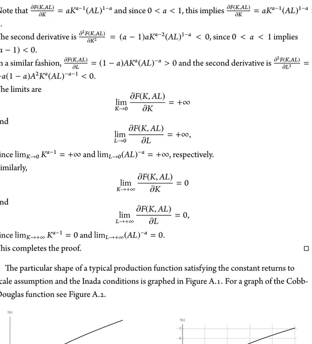
A.1 Plot of a typical production function satisfying the constant return to scales as-sumption and the Inada conditions. . . 44
A.2 Plot of Cobb-Douglas f(k)= k12. . . 44
B.1 Population Growth Data. . . 48
Listing of tables
3.1 Simulation Input Data. . . 28
3.2 Summary of scenarios to be simulated - Initial Values & Changes. . . 30
3.3 Simulation Results. . . 34
3.4 Convergence Results. . . 36
Listing of symbols
Symbol Description
∀ ”For all”
x := y ”x is defined to equal y”
P =⇒ Q ”P implies Q” or ”If P, then Q”
P ⇐⇒ Q ”P if and only if Q” or ”P is equivalent to Q”
x∈ X ”x is an element of the set X”
f : X→ Y ”The function f from the set X into the set Y”
x7→ f(x) ”x maps to f(x)”
limx→af(x)= l ”The limit l of f as x approaches a”
∂f(x)
∂xi ”The derivative of f(x) with respect to xi”
∂2f(x)
∂x2
i ”The second derivative of f(x) with respect to xi”
∫
f(t) dt ”The indefinite integral of f”
∫b
a f(t) dt ”The definite integral of f from a to b”
maxxi,yjf(xi, yj) ”The maximization problem of f with constraints xi and yj”
Acknowledgments
I am indebted for many valuable advices and suggestions to Johan Lindén, who has read a variety of iterations of this paper and has guided me with great care. On a more professional level, I am indebted to many great men who have laid the foundations for the immense body of knowledge, which represents the greatest achievement of the human intellect, of which without, this paper would have not been possible. I am grateful to be standing on the shoul-ders of giants.
Everything starts somewhere, although many physicists disagree.
T. Pratchett
0
Introduction
T
he magnum opus of the Scottish economist and moral philosopher Adam Smith is un-doubtedly his monumental work on the treatise of economic wealth, titled ”An Inquiry into the Nature and Causes of the Wealth of Nations”. The Wealth of Nations was first published in 1776 and is a fundamental work in classical economics, being one of the world’s first col-lection of descriptions on a nation’s wealth. Economic theory enjoyed a substantial amount of development since the times of the classical economists Adam Smith, Jean-Baptiste Say, David Ricardo, Thomas Robert Malthus, and John Stuart Mill. The marginal revolution of the latter half of the 19thcentury transformed classical economics into what is now known as neo-classical economics. Prominent names such as John-Maynard Keynes, Alfred Marshal, and Irving Fischer have made significant contributions to this new era of economic thought.One of the quintessential devotions of neo-classical economics is to model the real world economy and capture its complex nature in a simple mathematical framework. Many such efforts have been proposed such as the Harrod-Domar model, the Solow-Swan model, the Ramsey-Cass-Koopmans model, and the Romer model. Arguably the greatest achievements on the frontier of economic growth theory are the Solow-Swan model and the Romer model.
Problematization
Given that there are two groundbreaking papers on economic growth theory, one bySolow
(1956) and the other byRomer(1990), a natural question arises: ”Which model is more adequate for the purpose of analyzing different economic scenarios using a simulated envi-ronment?”. In particular, given the limitations below, the prior question is further limited by simulating the economies along a partial transition dynamics only rather than along the complete transition dynamics.
An auxiliary enquiry which is in conjunction to the a priori mentioned problematization is: ”Which values for the parameters are ’reasonable’ choices?” - and shall be investigated in this report as well.
The final problem which this paper will analyze is the speed of convergence from one steady-state to the new steady-state within both models.
A Brief Treatment On Economic Growth Theory
The age-old problem of economic growth theory has preoccupied economists for centuries. This phenomenon fascinated the classical economists so strongly that it gave birth to the famous treatise ”An Inquiry into the Nature and Causes of the Wealth of Nations” (Smith,
1963). However, the defeats of classical economic thought in the early 19thcentury such as
the mistaken forecast of Thomas Robert Malthus earned the discipline ”its most recognized epithet, the ’dismal science.’” (Jones & Vollrath,2013, p. 1).
A revolution on the frontier of economic thought was emerging in the latter half of the 19thcentury1. This period is usually referred to as the ”marginal revolution”2and it marks the transition from classical economics to neo-classical economics. This new era of economic thought brought forth a wide range of development to the old problem of economic growth theory. The Solow-Swan model of economic growth, and its many extensions, lie at the heart of modern growth theory (Halsmayer & Hoover,2016).
Although more modern considerations of the historical development suggest an attribu-tion to the Harrod–Domar model (Blume & Sargent,2015), a central point of criticism is
1It is difficult to accurately pin-point the precise date.
2As a matter of fact, it is argued whether this period should be referred to as the ”utility revolution” or as a
that Harrod’s original work, ”Essay in Dynamic Theory” (Harrod,1939), was neither mainly concerned with economic growth3, nor did he explicitly use a fixed proportions production
function (Besomi,2001).
The Solow-Swan model is not a singular achievement in economic growth theory. Two models that resemble the Solow-Swan model are the Ramsey-Cass-Koopmans model and the Diamond model. Of which in both, the dynamics of economic aggregates are determined by decisions at the microeconomic level and both models continue to treat the growth rates of labor and knowledge as exogenous (Romer,1996). However, both models derive the evolution of the capital stock from the interaction of maximizing households and firms in competitive markets and as a result the saving rate is no longer exogenous and it need not be constant. A major difference between the Ramsey-Cass-Koopmans model and the Diamond model is the key additional assumption in the latter, that there is continual entry of new households into the economy, which has important consequences (Romer,1996).
Following the successes of Robert M. Solow from the 1950s, the work on economic growth flourished during the 1960s and 1970s, with the works of economists like Moses Abramovitz, Kenneth Arrow, David Cass, Tjalling Koopmans, Simon Kuznets, Richard Nelson, William Nordhaus, Edmund Phelps, Karl Shell, Eytan Sheshinski, Trevor Swan, Hirofumi Uzawa, and Carl von Weizsacker (Jones & Vollrath,2013). Nevertheless, the prior mentioned investigations have not explored the nature of technological change andRomer
(1994) provides methodological reasons for this postponement.
It was Paul Romer and Robert Lucas who revitalized the interest of macroeconomists in economic growth in the early 1980s by introducing the economics of technology (Jones & Vollrath,2013). New growth theory transcends beyond the Solow-Swan model with mod-els like the research and development growth modmod-els developed by P. Romer, Grossman and Helpman, and Aghion and Howitt (Romer,1996). Models of endogenous growth are not the only modern considerations of examining economic growth but also models of
hu-3To quote from (Blume & Sargent,2015, p. 352): ”Harrod himself did not emphasize the contribution to
economic growth.”.
And further: ”Although Harrod’s article seems partly about economic growth, most economists today have been convinced by Solow’s and Swan’s claim that labour–capital substitutability was the pertinent as-sumption for a long-run analysis and their demonstration that using that asas-sumption in place of Harrod’s fixed-co-efficient model of investment pulls the rug out from under Harrod’s distinction between a natural and warranted growth rate.”.
man capital and growth developed byMankiw et al.(1992) have been proposed in order to analyze the cross-sectional growth between countries.
Even though the field of growth theory has flourished over the past century and many new ideas and extensions of old ideas have been developed and investigated, it is clear that neo-classical growth theory began with the key insight of one man: Robert M. Solow, and the revitalization of modern growth theory is attributed to Paul Romer.
Purpose
The purpose of this thesis is to compare the Solow-Swan model with the Romer model using numerical data within a simulated environment. The derivation of the necessary economic re-lations shall be executed using a non-standard economic style, that is, using the mathematical Axiom-Definition-Proposition style.
The differences between the two a priori mentioned models will be undertaken by an investigation of five simulated experiments. The purpose of the experiments is to illuminate the implications of different changes in variables and give insights into the necessary choices for the values of the variables which are used within simulations utilizing the Solow-Swan model and the Romer model.
The first experiment investigates a change in the saving rate. Experiment two analyzes the effects of a change in the population growth. The third experiment illustrates the scenario of a decrease in the output elasticity of capital. Experiment number four considers an alteration in the depreciation rate. The fifth and final experiment investigates modifications to both, the population growth and saving rates. Each of the scenarios will be more elaborated in Chapter 3.
Lastly, the final purpose of the experiments is to enable the performance for the analysis of the speed of convergence between steady-states.
Methodology
As mentioned above, the two growth models under investigation in this paper are the Solow-Swan model and the Romer Model. The following methodology for the theoretical and numerical analysis shall be applied.
• Propose the axioms4for the two growth models under consideration.
• Deduce necessary propositions by means of rigour from the prior mentioned axioms. • Gather data for input into simulation. The majority of the data will be given from
different economies such as the saving rate of different countries or the population growth of different countries. This point will be further elaborated in Chapter 3. • Simulate five different economic scenarios over a given period of time and evaluate the
results.
• Propose a method for analyzing the speed of convergence between steady-states. The above methodology will become clearer throughout the upcoming chapters. The economic scenarios will be referred to as experiments.
The data used as inputs into the simulations was gathered by each governmental statistical agency within the nation under consideration. In Sweden the agency responsible for gather-ing economic data is called Statistics Sweden (SCB) and in the United States it’s the Bureau of Economic Analysis (BEA). The data was received fromWorld Bankand the data which was used for the purposes of this investigation is summarized in Appendix B.
Limitations
This paper simulates the models on a balanced growth path and partly on the transition dy-namics. The only transition dynamics which shall be considered is that of the capital per effective worker. The reason for this choice is the time constraint which is set by the course description and also that the complexity of the complete transition dynamics simulation is far greater than that of the consideration in this paper. Hence, if the reader is interested in the complete transition dynamics, then this report will not satisfy that interest.
A second limitation is the underlying nature of the term ’model’. A model is a simple ap-proximation of a complex phenomenon and is (most likely) not able to capture the entire complexity of the phenomenon under investigation. Nevertheless, even such simple ap-proximations of the world are capable of illuminating intriguing problems. This limitation is
4Usually within the subject of economics the term ’assumption’ is used rather than ’axiom’. However, I
however not singular to this paper alone and is rather a general ”weakness” of modelling the complexity of the world and it perhaps belongs within the realms of philosophy.
It is quite wrong to try founding a theory on observable magnitudes alone. ... It is the theory which decides what we can observe.
Albert Einstein
1
The Solow-Swan Model
T
he Solow-Swan growth model1, is a neo-classical economic growth model which was independently developed by Robert M. Solow, published inSolow(1956), and by Trevor Winchester Swan, published inSwan(1956). This most beautiful and simultaneously simplis-tic mathemasimplis-tical framework, which lies at the front of many extensions, has earned Robert M. Solow the Nobel price in economics for its fundamental rˆole in economic growth theory and its impact on the discipline.Definition And Solow Postulates
Definition 1.1. The Solow Growth Model consists of a production function Y(t) together with a set of axioms (Si) called the Solow Postulates. Let Y(t) be output, K(t) capital, L(t) labor and A(t) knowledge. Then, the aggregate production function F : R2
+ → R such that
(K(t), L(t)) 7→ Y(t) at time t is defined by
Y(t) := F(K(t), A(t)L(t)). (1.1)
Axioms 1.2. Solow Postulates.
(S1) Constant returns to scale. The production function Y = F(K, AL) as given by
Defin-tion 1.1 has constant returns to scale. In other words, let ζ ∈ R≥0, then
F(ζK, ζAL) = ζF(K, AL). (1.2)
(S2) Two factor inputs: Labor & Capital. Factor inputs to the production function such
as land and other natural resources are negligible.
(S3) Time is continuous. The model assumes continuous time in the sense that the
vari-ables are defined at every point in time2.
(S4) Inada conditions3. The production function satisfies the Inada conditions. Let f : Rn+ → R such that x 7→ f(x) be a continuously differentiable function4. Then, the conditions are
(i) If x = 0, then f(x) = 0.
2This assumption simplifies the mathematical analysis. An alternative assumption is to assume discrete
time, that is, the variables are defined at specific time intervals t = 0, 1, 2, .... However, the Solow model has essentially the same implications in discrete as in continuous time (Romer,1996, p. 11).
3These conditions are named after Ken-Ichi Inada fromInada(1963) and were first introduced by H.
Uzawa inUzawa(1963).
4Boldface objects denote vectors such that x∈ Rnis the vector (n-tuple) x= (x
1, ..., xn) with xi∈ R and
Rnis the real vector space consisting of all n-tuples. A concise treatment of vector spaces can be found in
(ii) The function f is concave5on its domain. In other words, the marginal returns for inputs xiare positive6such that∂f(x)∂xi > 0, but decreasing such that∂
2f(x)
∂x2
i < 0. (iii) As xiapproaches zero, the limit of the first derivative is positive infinity such that
lim xi→0
∂f(x) ∂xi
= +∞.
(iv) As xiapproaches positive infinity, the limit of the first derivative is zero such that lim
xi→+∞ ∂f(x)
∂xi = 0.
(S5) Labor and knowledge are exogenous7and grow at constant rates. Let L(0) := L0
and A(0) := A0be the initial values of labor and knowledge, respectively. I.e. their
values at time t0= 0. Furthermore, let n, g ∈ R≥0be the growth rates of labor and
knowledge, respectively. Then8, ˙L(t) := nL(t) =⇒ ∫ ˙L(t)dt= ∫ nL(t)dt ⇐⇒ L(t) = L0ent, (1.3) ˙ A (t) := gA(t) =⇒ ∫ ˙ A (t)dt= ∫ gA(t)dt ⇐⇒ A(t) = A0egt, (1.4) (S6) Change in capital & the saving rate. Each period, a fraction of the outcome is saved
and invested in physical capital. Furthermore, the physical capital K(t) depreciates each period. Let δ, sK ∈ R such that δ ≥ 0 and 0 < sK< 1 be the depreciation rate and the saving rate, respectively. Then, the change in capital stock ˙K (t) is
˙
K (t) := sKY(t)− δK(t). (1.5)
5For a lucid treatment on concavity and convexity, seeSpivak(1994). 6This condition is known as the semi-definiteness of the Hessian matrix H
i, j:= ( ∂2f ∂xi∂xj ) (Takayama,1985, 125–126).
7An exogenous variable is a variable which is not explained by the model itself in the sense that it is
deter-mined by outside forces. Contrary, an endogenous variable is a variable which is explained by the model.
8Here, ˙X (t) denotes the derivative with respect to time such that ˙X (t) :=dX(t)
dt . This notation was
Romer(1996) remarks that time only enters the production function through changes in capital, labor, or knowledge, and thus, henceforth we will not use the independent vari-able t in equations unless necessary. Furthermore, the product AL is known as the labor-augmenting or Harrod-neutral technological progress9.
Romer(1996) also mentions that focusing on the per unit of effective labor measurement
1
ALis more convenient. Thus, the production function can be written in the following more concise form.
Proposition 1.3. The production function can be written in the intensive-form10
˜y = f(˜k), (1.6)
where we define ˜k := K AL, ˜y :=
Y
AL, and f(˜k) := F(˜k, 1).
Proof. By substituting ζ = AL1 into equation 1.2, it follows from Axiom 1.2 (S1) that
F(ζK, ζAL) = ζF(K, AL), (1.7)
which in turn implies
F ( K AL, 1 ) = 1 ALF(K, AL). (1.8)
Hence, equation 1.8 becomes ˜y= f(˜k). □
9Technological progress of the form AK is called capital-augmenting and technological progress of the
form AF(K, L) is referred to as Hicks-Neutral (Romer,1996, p. 17).
Dynamics Of The Model
Axioms 1.2 imply the following dynamics of the Solow model.
Proposition 1.4. The dynamics of the capital stock per unit of effective labor ˜k= ALK is given by the differential equation11
˙˜k = sKf(˜k)− (n + g + δ)˜k. (1.9) Proof. Since ˜k= K AL, we have ˙˜k = K˙ AL − K AL ˙ A A − K AL ˙L L. (1.10)
Now, ˜k= ALK. By 1.4, AA˙ = g, by 1.3, L˙L = n, and by 1.5 ˙K = sKY− δK. Thus, 1.10 becomes ˙˜k = sKY
AL − δ˜k − g˜k − n˜k. (1.11)
And since f(˜k)= ALY , equation 1.11 becomes
˙˜k = sKf(˜k)− (n + g + δ)˜k,
as desired. □
The steady-state ˜k∗is given by the value of ˜k at˙˜k = 0. Since ˜k converges to ˜k∗, it converges to a balanced growth path12, in which the growth rate of output per worker is determined
solely by the rate of technological progress (Romer,1996, pp. 17–18). Thus, we make the following definition.
Definition 1.5. The steady-state value of capital per effective worker ˜k∗is defined by the value of ˜k at˙˜k = 0. Furthermore, a balanced growth path is a path (Y, K, C)∞t=0along which the quantities Y, K, and C are positive and grow at constant rates13.
11For an introductory treatment on differential equations, DE for short, seeApostol(1969). 12The balanced growth path is the scenario in which the model grows at constant rate.
13The quantity C stands for aggregate consumption. In the Solow model, C is used to define aggregate
A simple - yet beautiful - production function which satisfies the constant returns to scale assumption and the Inada conditions14is the Cobb-Douglas15production function F :R2
+→ R such that (K, L) 7→ Kα(AL)1−αdefined by
F(K, AL) := Kα(AL)1−α, ∀α ∈ R : 0 < α < 1. (1.12) Before proceeding, we shall decide on the form of the production function. We shall choose the Cobb-Douglas production function as defined by equation 1.12. Writing the Cobb-Douglas function as per effective worker16yields f(˜k)= ˜kα.
Thus, Proposition 1.4 holds the following corollary.
Corollary 1.5.1. Within the Solow model, the steady-state of capital per effective worker is given by the relation
˜k∗= ( sK
n+ g + δ
) 1 1−α
. (1.13)
Furthermore, the steady-state value of output per effective worker ˜y∗is given by
˜y∗= ( sK n+ g + δ ) α 1−α . (1.14)
Proof. By Proposition 1.4, we have˙˜k = sKf(˜k)− (n + g + δ)˜k. The Cobb-Douglas function is
f(˜k)= ˜kαand by Definition 1.5 we have to solve˙˜k = 0. Thus, ˜k∗= ( sK n+ g + δ ) 1 1−α .
Substituting 1.13 into f(˜k)= kαyields equation 1.14, as desired. □
14A proof of this fact is given in Appendix A, Proposition A.1.
15Named after Charles Cobb and Paul Douglas which appeared inCobb & Douglas(1928). 16The derivation of this fact is left to the reader.
Every generation has underestimated the potential for finding new ideas.
Paul Romer
2
The Romer Model
P
aul M. Romer proposed a mathematical theory of endogenous growth of new ideas inRomer(1990). This was a remarkable achievement in illuminating the nature of technologi-cal progress. However,Jones(1995) argues that the prediction of many recent research and development models of growth are inconsistent with the time-series evidence from industri-alized economies1. In particular,Jones & Vollrath(2013) remark that Romer assumes that
the productivity of research is proportional to the existing stock of ideas. This means that the productivity of researchers grows over time, even if the number of researchers is constant. Furthermore, the original formulation given byRomer(1990) predicts that the growth rate of the advanced economies should have risen within the past forty years, since the amount of world research efforts has risen. Despite all this,Jones(1995) investigation shows that this is far from the truth. In spirit of this discussion, the version of the Romer model which we shall treat here is the one given byJones(1995).
1To be more precise, Jones himself writes: ”Romer(1990) and others share the counterfactual prediction
of ’scale effects’: an increase in the level of resources devoted to R & D should increase the growth rate of the economy.” (Jones,1995, p. 761).
Definition And Romer Postulates
Definition 2.1. The Romer Growth Model consists of three sectors. The final-goods sector, the intermediate-goods sector, and the research sector, together with a set of axioms (Ri) called the Romer Postulates.
Let Y be output, K the stock of capital, LYlabor used in producing output, and A the stock of ideas. Then, we define the aggregate production function2within the Romer economy F :R3
+→ R such that (K, A, LY)7→ Y by
Y := F(K, A, LY). (2.1)
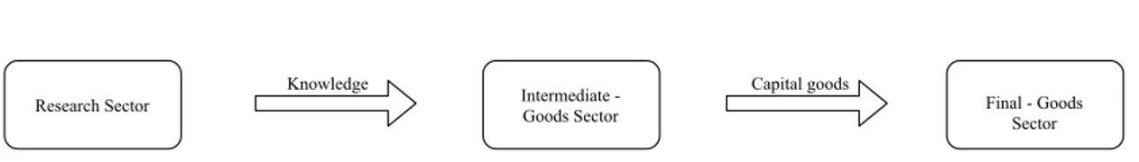
A diagrammatic representation of the relationship between the three sectors is given by Figure 2.1.
Axioms 2.2. Romer Postulates.
(R1) Increasing returns to scales by A. Given how ideas differ from ordinary economic
goods3we assume increasing returns to scales. In other words, for ζ ∈ R
≥0we have
F(ζK, ζA, ζLY)> ζF(K, A, LY).
(R2) Labor and depreciation are exogenous. As within the Solow model, participants of
the economy save a fraction of income sKand capital depreciates at an exogenous rate
δ such that the change in capital ˙K is
˙
K := sKY− δK. (2.2)
In parallel to the Solow model, labor grows at a constant exogenous rate n such that the change in labor ˙L is
2As we shall later see, the production function takes the form Y= Kα(AL
Y)1−αas given by Proposition
2.13.
3Technology, that is, new ideas, designs, or scientific research are non-rivalrous, partially-excludable
goods. A purely rivalry good is the idealization that a good has the property that its use by one firm or per-son precludes its use by another. A good is excludable if the owner can prevent others from using it. It then helps to think that a new idea or design can be used over and over again once it has been created and it is partially excludable because there are methods by which one can prevent its use by others. Such methods could possibly be patents. A more detailed treatment of these concepts is given inRomer(1990).
˙L := nL, (2.3) where labor L is divided between labor used within the final-goods sector LYand labor used for the creation of new ideas in the research sector LAsuch that
L := LY+ LA.
(R3) Technology is endogenous. Let θ, λ, φ ∈ R such that θ and φ are constants and 0 < λ < 1 is a parameter. The number of new ideas produced ˙A at any given point in time
is given by the production function for new ideas4 ˙
A := θLAλAφ. (2.4)
Knowledge
Research Sector Intermediate Goods Sector
Capital goods
Final Goods Sector
Figure 2.1:Diagramma c representa on of the three sector Romer model.
The research sector uses human capital and the existing stock of knowledge to produce new knowledge/designs.
The intermediate-goods sector uses the designs (ideas) from the research sector to produce the producer durables (capital goods) which are used in the final-goods sector.
The final-goods sector uses labor, human capital, and the set of capital goods from the intermediate-goods sector to produce final output.
4Using the special case λ = φ = 1 reduces ˙A to the case of the originalRomer(1990) model. Furthermore,
The Final-Goods Sector
The final-goods sector of the Romer economy reflects the final-goods sector of the Solow model. Thus, we have the following additional axiom.
Axioms 2.3. Romer Postulates - Final-Goods Sector.
(R4) Let Y be output, LYlabor used in producing output, and x := (xi)∞i=1the sequence of different capital goods5to be used in producing final output. Then, we define the production function Y such that (LY, (xi)∞i=1) 7→ L1−αY
∑∞
i=1xαi within the final-goods sector by Y := L1−αY ∞ ∑ i=1 xαi.
As remarked byJones & Vollrath(2013), it is easier to analyze the model if the summation is replaced by an integral such that
Y= L1−αY ∫ A
0
xαidi, (2.5)
where A measures the range of capital goods that are available to the final-goods sector over the closed interval [0, A] := {x ∈ N : 0 ≤ x ≤ A}.
Firms in the final-goods sector have to decide how much labor and how much of each capital good to use in producing output. Let πFbe the total profit of the final-goods sector,
pithe rental price for capital good i and wYthe wage paid for labor. Then, microeconomic theory formulates the following problem
πF= L1−αY ∫ A 0 xiαdi− wYLY− ∫ A 0 pixidi, which in turn becomes the profit-maximization problem
max LY,xi πF= max LY,xi L1−αY ∫ A 0 xαidi− wYLY− ∫ A 0 pixidi.
5In fact, there is some value A∈ Z
This leads to the following proposition, of which its results are used within the next sector, that is, the intermediate-goods sector.
Proposition 2.4. The profit-maximization problem for the final-goods sector implies the following.
(i) Firms hire labor until the marginal product of labor equals the wage such that
wY = (1 − α)
Y LY
. (2.6)
(ii) Firms rent capital goods until the marginal product of each kind of capital equals the rental price pi. In other words, the demand function for capital goods is given by
pi = αL1−αY xiα−1. (2.7)
Proof. (i) We have to solve∂πF
∂LY = 0. Thus, ∂πF ∂LY = (1 − α)L−α Y ∫ A 0 xαidi− wY = (1 − α)L−1+1−α Y ∫ A 0 xαidi− wY = 0.
Hence, by equation 2.5 we have
(1− α)L−1Y Y− wY = 0 ⇐⇒ wY= (1 − α)
Y LY
. (ii) Similarly, solving∂πF
∂xi = 0 yields
αL1−αY xαi − pixi = 0 ⇐⇒ pi = αL1−αY xαi−1.
The Intermediate-Goods Sector
The intermediate-goods sector consists of monopolists who produce the capital goods that are sold to the final-goods sector. Once the design for a particular capital good has been pur-chased, the intermediate-goods firm produces the capital good with a very simple production function: one unit of raw capital can be automatically translated into one unit of the capital good (Jones,1995). The profit maximization problem for an intermediate goods firm is then
max xi
πi = max xi
pi(xi)xi− rxi, (2.8)
where piis the demand function from the final-goods sector for capital goods given by equation 2.7.
Proposition 2.5. The profit-maximization problem for the intermediate-goods sector implies
p = 1
1+ p′(x)xp r. (2.9)
Proof. Solvingdxdπi = 0 yields
0= p′(x)x+ p − r ⇐⇒ p + p′(x)x= r ⇐⇒ ( 1+ p ′(x)x p ) p= r ⇐⇒ p = 1 1+ p′(x)xp r. □ Proposition 2.5 holds the following corollary.
Corollary 2.5.1. All capital goods are sold for the same price by each monopolist by
p = 1
αr. (2.10)
Proof. From 2.7 we can calculate the elasticityp′(x)xp such that
Hence,
p′(x)x
p =
(α− 1)αL1−αY xα−2x
αL1−αY xα−1 = (α − 1). Substituting into 2.9 yields
p = 1 αr,
as desired. □
Jones & Vollrath(2013) remark that the demand functions from Proposition 2.4 (ii) equa-tion 2.7 are the same for each firm. This means that each capital good by the final-goods firms is employed in the same amount xi = x. This leads to the following result.
Proposition 2.6. Each capital-goods firm earns the same profit given by
π = α(1 − α)Y
A. (2.11)
Proof. By 2.8 and 2.7 we have
π = αL1−αY xα− rx,
and by 2.10 this becomes
π = αL1−αY xα− αpx = αL1−α Y xα− ααL1−αY xα = αL1−α Y xα(1− α). (2.12)
Now, from equation 2.5, Y= L1−αY ∫0Axα
Y= L1−αY ∫ A 0 xαdi = L1−α Y xαi A 0 = L1−α Y xαA. Hence, YA = L1−αY xα. Thus, 2.12 becomes
π = α(1 − α)Y A
□ (Jones,1995) The total demand for capital from the intermediate-goods firms must equal the total capital stock in the economy such that
∫ A 0 xdi= K ⇐⇒ xi A 0 = K ⇐⇒ xA = K ⇐⇒ x = K A.
This result gives the form of the final-goods production function.
Proposition 2.7. The final-goods production function from 2.5 can be re-written such that
Y= Kα(ALY)1−α. (2.13) Proof. We have Y= L1−αY ∫0Axαdi= L1−α Y xαi A 0 = L1−α
Y xαA and since x= KA, this implies
Y= Kα(ALY)1−α.
□
The Research Sector
Ideas are designs for new capital goods to be sold to the intermediate-goods sector and are generated according to the production function for ideas give by equation 2.4. Let r be the
in-terest rate and PAthe price of a new design, this present discounted value. Then, the arbitrage equation is
rPA = π + ˙PA ⇐⇒ PA=
π
r− n. (2.14)
This equation gives the price of a patent along a balanced growth path and is used in the next section to derive the relation for the share of the population which is engaged in re-search, as given by Proposition 2.10.
Dynamics Of The Model
Let y and k be per capita output and capital-labor ratio, respectively. Furthermore, let gy, gk, and gAbe the growth rates of per capita output, capital-labor ratio and technology along a balanced growth path. Then, the growth rates must be the same6such that7
gy = gk= gA.
Recalling from Definition 1.5 that along a balanced growth path the growth rates are con-stant and in particular that gA:=
˙
A
A is constant, we have the following proposition. Proposition 2.8. The long-run growth rate of the Romer economy is determined by the parameters of the production function for ideas and the rate of growth of researchers such that
gA =
λn
1− φ. (2.15)
Proof. From Axiom (R3) equation 2.4 we have
gA = ˙ A A = θL λ AAφ−1. (2.16)
6This result is derived inJones & Vollrath(2013) and it implies that if there is no technological progress,
then there is no economic growth.
7It is also worth mentioning thatJones(1995) introduces a new term of ”semi-endogenous” growth. The
reason for this choice is that in the model proposed byJones(1995) the tranditional policy changes have no long-run growth effects as in theRomer(1990) and AK models. Jones himself writes: ”Long-run growth rate is a function of parameters usually taken to be invariant to government policy” (Jones,1995, p. 761). Here, invariance of governmental policies refers to steady-state growth from government tax policy, including investment tax credits and R & D subsidies.
Differentiating both sides8with respect to t and noting that gAis constant on a balanced growth path as given by Definition 1.5, yields
0= λθLλA−1˙LAAφ−1+ (φ − 1)θLλAAφ−2A˙ = λθLAλAφ˙LA LAA + (φ− 1)θLλAAφA˙ A2 = λ ˙A ˙LA LAA + (φ− 1) ˙A ˙A A2 . Since gA= ˙ A
A and by recognizing that along a balanced growth path the growth rate of the number of researchers must be equal to the growth rate of the populationJones & Vollrath
(2013), it follows from Axiom (R2) equation 2.3 that
0= λn ˙A + (φ − 1) ˙AA˙
A
= λn ˙A + (φ − 1) ˙A gA. Which in turn is equivalent to
gA(φ− 1) ˙A = −λn ˙A ⇐⇒ gA= −λn ˙A (φ− 1) ˙A = −λn (φ− 1) = λn (1− φ), as desired. □
It is worth mentioning that in this economy the long-run growth rate of technology gA as given by Proposition 2.8 equation 2.15 is invariant to investment and the number of re-searchers from the population which are engaged in research. Proposition 2.10 below illus-trates the relation which gives the share of the population that is engaged in research.
Furthermore, notice that if φ = 1 as in theRomer(1990) model, then equation 2.15 is undefined9. This means that if we allow for φ to be one, then there is no balanced growth
8An alternative way would be to take logs on both sides and then differentiate with respect to t asJones &
Vollrath(2013) present. However, such petty tricks only cripple the intellect.
9This is because we are using the algebraic field (R, +, ∗), in which division by 0 will break some
path within this economy. Thus, the assumption that φ< 1 as mentioned byJones(1995) removes the scale effects which are not supported by time-series evidence and replaces it with the intuitive dependence on the growth rate of the labor force rather than on its level. Proposition 2.9. The Romer Postulates imply the following conditions.
(i) The per-effective labor production function is given by
˜y= ˜kα(1− sR)1−α, (2.17)
where sRis a constant fractionLLA := sRof the labor force that engages in research and development.
(ii) The dynamics in the Romer economy is given by the relation
˙˜k = sK˜kα(1− sR)1−α − (n + gA+ δ)˜k. (2.18) (iii) The steady-state capital per effective worker is
˜k∗ = ( sK n+ gA+ δ ) 1 1−α (1− sR). (2.19)
(iv) The steady-state output per effective worker ˜y∗is given by
˜y∗= ( sK n+ gA+ δ ) α 1−α (1− sR). (2.20)
Proof. By Proposition 2.7, Y= Kα(AL
Y)1−αand since ˜y= ALY = Ay andLLY = 1 − sR, we have ˜y = ˜kα(1− sR)1−α,
which proves (i).
˙˜k = K AL˙ − K( ˙A L + A ˙L) (AL)2 = K˙ AL − K ˙A A2L − K ˙L AL2.
By Axiom (R2) equation 2.2, ˙K = sKY− δK, equation 2.3, ˙L(t) = nL(t), and
˙ A A = gA. Thus, ˙˜k = sKY− δK AL − K ALgA− K ALn = sK Y AL − δ K AL − K ALgA− K ALn which is equivalent to ˙˜k = sK˜y− (n + gA+ δ)˜k = sK˜kα(1− sR)1−α− (n + gA+ δ)˜k, and hence proves (ii).
Using (ii) and solving for the steady-state˙˜k = 0 as indicated by Definition 1.5, yields
˜k∗= ( sK n+ gA+ δ ) 1 1−α (1− sR). This proves (iii).
Now, substituting 2.19 into 2.17 yields
˜y∗= ( sK n+ gA+ δ ) α 1−α (1− sR), as desired. □
What remains to be derived is the expression for the share of the population that works in the research sector sR.
Proposition 2.10. The share of the population that works in the research sector sRis deter-mined by
sR = 1 1+ rαg−nA
It doesn’t matter how beautiful your theory is, it doesn’t matter how smart you are. If it doesn’t agree with experi-ment, it’s wrong.
Richard P. Feynman
3
Simulations
I
n this chapter the experimental simulations of the different economic scenarios are presented. In the first section of this chapter, a discussion of the choices of the values for the variables which are used for the purposes of the experiments will occur. These particular values are summarized in Appendix B Table B.1. In the second section, each experiment will be elaborated in detail, that is, the initial conditions and the occuring change(s) shall be explained. The third section will present each simulated experiment and the implications which arise by each model will be analyzed. Lastly, the final section will consider the speed of convergence for the output per effective worker ˜y and capital per effective worker ˜k within both models.Choosing Parameter Values
For the production function we choose for the majority of the experiments a value of α= 0.33 as investigated byCobb & Douglas(1928). We will however allow ourselves more freedom in tweaking α in some experiments. More on this later.
Now, we discuss the parameter and variable choices for the Solow model from Chapter 1. From the Solow Postulates 1.2 the exogenous variables are the saving rate s, the growth rate of labor n, the growth rate of knowledge g, and the depreciation rate of capital δ. For the saving rate s we choose data from different countries and similarly for n, we choose the growth rate of population from different countries which both are given in Appendix B Tables B.1 and B.2. The mean values of the prior mentioned population growth and saving rates are sum-marized in Table 3.1, which will also give the ranges of the parameter values in which we will operate.
According to the Swedish Tax AgencySkatteverket, annual depreciation of machinery and other equipment is allowed at 30 percent of the residual value or at 20 percent of the acquisition value. Buildings are depreciated by 2 to 5 percent per year depending on their use. Thus, for the depreciation rate δ, we choose a value between 0.02 and 0.2.
According toMankiw(2013) the economies of Japan and Germany have experienced one of the most rapid growth rates ever recorded. These values are 8.2 percent and 5.7 percent per year after the events of World War II destroyed most of their capital stock. The United States of America had a very constant growth rate of 2.2 percent per year. For these reasons, the technology growth g will range between 0.01 and 0.05, since rapid growth rates such as the postwar ones are unreasonable for advanced economies.
For the Romer model, in addition to the variables which are in the Solow economy, there are other parameters which have to be taken into consideration. These are λ, φ, and the dis-count rate r. The values chosen for these parameters are done in such a way as to approxi-mate the endogenous technological growth rate in the Romer model gAwith the exogenous growth rate of technology from the Solow model g. The reason for this choice is that we can approximate as accurately as possible the initial conditions in both models with which the economies start, before the experimental changes occur. Furthermore, this enables to pro-duce a ”fair”1comparison between the two models.
It is worth mentioning that the reported value of the share of the population engaged in research byUNESCOis 0.1 percent of the global population andOECD(2018) report a value of 8.29 per thousand employed. Furthermore, theFederal Reservereports a discount rate of 2.5 percent. However, we will not restrict ourselves to these numerical values since it is more important to approximate the technological progress in the Romer model with that of the Solow model for reasons mentioned above.
For the purposes of accessibility, the values of the variable ranges are summarized in Ap-pendix B Table B.1.
Mean Values
Country Name Mean Population Growth Mean Saving Rate
China 0.013057976 0.43 European Union 0.003977026 0.22 Germany 0.002325561 0.24 India 0.019296831 0.28 Japan 0.00571623 0.28 Romania 0.001336249 0.20 Russian Federation 0.003513161 0.28 Sweden 0.005065072 0.27 Switzerland 0.008310902 0.34 United States 0.010498057 0.20 World 0.016172349 0.24 Range 0.001336249 - 0.019296831 0.20 - 0.43
Table 3.1:Simula on Input Data.
Experiments
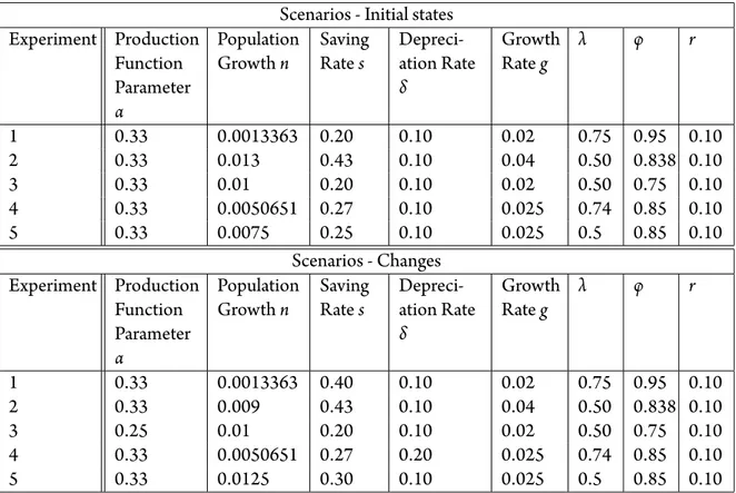
We consider five simulated experiments. Each of the experiments will be briefly discussed and are summarized in Table 3.2. Each economy begins in a steady-state from time period t0
= 0 until period t = 5. During period t = 5 certain changes to the models will occur. Table 3.2 summarizes the occuring changes.
Experiment 1 - An increase in the saving rate. Economy 1 starts in the steady-state with an output elasticity of capital α= 0.33, a population growth rate n = 0.00134, a saving rate
in period t= 5 to the value of the endogenous technological growth rate gA. This however will only impact
the actual values within the Solow model and not its core implications. However, in the ”Speed Of Conver-gence” section of this chapter, these adjustments shall be performed. More on this later.
s= 0.20, a depreciation rate δ = 0.1, and a technological rate of g = 0.02. The choices of the
forehand mentioned values reflect an economy such as that of Romania. Let us suppose that during period t= 5 a new governmental policy is proposed which increases the saving rate to
s= 0.4.
Experiment 2 - A decrease in the population growth. Economy 2 begins in the steady-state with an output elasticity of capital α= 0.33, a population growth rate n = 0.013, a saving rate
s= 0.43, a depreciation rate δ = 0.1, and a technological rate of g = 0.04. This experiment
reflects an economy such as China. Let us suppose that during period t= 5 the government of economy 2 proposes a policy which decreases the population growth rate to n= 0.009. Such a possible policy could perhaps be the one-child policy which was adopted by China2in
the year 1979.
Experiment 3 - A change in the parameter α. In this experiment, we consider the scenario in which the parameter α of the production function decreases in period t = 5. In particular, α will be set from its initial value of 0.33 to 0.25.
Experiment 4 - A change in the depreciation rate. This experiment considers the change in the depreciation rate δ. Let us suppose that the initial values of the economy under con-sideration are that of Sweden which are summarized in Table 3.1. Furthermore, we assume a technological growth rate g= 0.025, a value of α = 0.33 and the initial value for the deprecia-tion rate will be δ= 0.1. During period t = 5 the depreciation rate will be set to 0.20.
Experiment 5 - An increase in the saving rate and an increase in the population growth rate. The fifth and final experiment considers a modification to two variables. To be more specific, a change in the saving rate sKand the population growth rate n. This is an interesting investigation since the mathematical equations show that these two forces have opposite ef-fects on capital per effective worker and output per effective worker when both are increased or both are decreased. Let us suppose the economy starts with values of α= 0.33, n = 0.0075,
sK= 0.25, δ = 0.1, g = 0.025, λ = 0.5, φ = 0.85, and r = 0.1. At t = 5 the values of n and sK increase to 0.0125 and 0.30, respectively.
2The one-child policy was then changed to a two-child policy in 2016. It is still a controversy whether or
not the one-child policy had any substantial impact on the population growth rate or the population size as found inWhyte et al.(2015) and inLi & Zhang(2006).
Scenarios - Initial states Experiment Production Function Parameter α Population Growth n Saving Rate s Depreci-ation Rate δ Growth Rate g λ φ r 1 0.33 0.0013363 0.20 0.10 0.02 0.75 0.95 0.10 2 0.33 0.013 0.43 0.10 0.04 0.50 0.838 0.10 3 0.33 0.01 0.20 0.10 0.02 0.50 0.75 0.10 4 0.33 0.0050651 0.27 0.10 0.025 0.74 0.85 0.10 5 0.33 0.0075 0.25 0.10 0.025 0.5 0.85 0.10 Scenarios - Changes Experiment Production Function Parameter α Population Growth n Saving Rate s Depreci-ation Rate δ Growth Rate g λ φ r 1 0.33 0.0013363 0.40 0.10 0.02 0.75 0.95 0.10 2 0.33 0.009 0.43 0.10 0.04 0.50 0.838 0.10 3 0.25 0.01 0.20 0.10 0.02 0.50 0.75 0.10 4 0.33 0.0050651 0.27 0.20 0.025 0.74 0.85 0.10 5 0.33 0.0125 0.30 0.10 0.025 0.5 0.85 0.10
Table 3.2:Summary of scenarios to be simulated - Ini al Values & Changes.
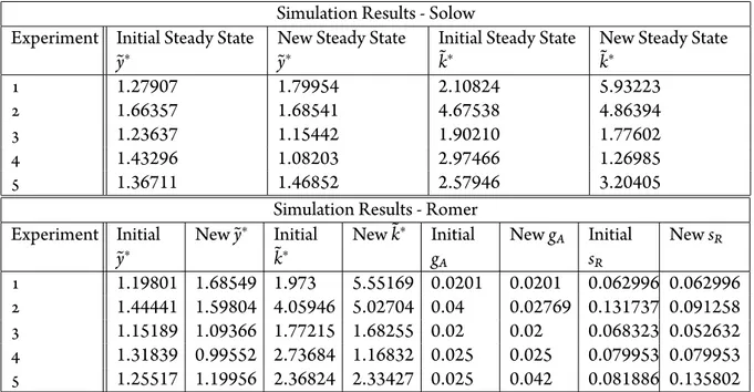
Simulation Results
The results of the simulations are summarized in Table 3.3. Before proceeding, some remarks must be made. As mentioned in the limitations section of Chapter 0, the transition dynamics will not be fully analyzed. This means that only the transition dynamics of the capital will be analyzed.
Experiment 1
Within the Solow economy, the initial steady-state values of output per effective worker and capital per effective worker are 1.279 and 2.108, respectively. Whereas in the Romer economy, the initial values are ˜y∗= 1.198 and ˜k∗= 1.973. The increase in the savings rate increases ˜y∗and ˜k∗in each of the models. In the Solow model, the new values are given by ˜y∗= 1.780 and ˜k∗= 5.932. In the Romer model we have ˜y∗= 1.686 and ˜k∗= 5.552. These changes are shown in Figures 3.1, 3.2, 3.3, and3.4. The results of this experiment are not
sur-prizing since an increase in the savings rate will result in a higher value of ˜y and ˜k in both models as the mathematical relations derived in the previous two chapters undoubtedly im-ply.
Figure 3.1:Experiment 1 - Output per effec ve worker - Solow.
Figure 3.2:Experiment 1 - Capital per effec ve worker - Solow.
Figure 3.3:Experiment 1 - Output per effec ve worker - Romer.
Figure 3.4:Experiment 1 - Capital per effec ve worker - Romer.
Experiment 2
A decrease in the population size will increase the new steady-states of output per effective worker and capital per effective worker in both models. The results are summarized by Fig-ures 3.5, 3.6, 3.7, and3.8. Although the results of this experiment are the same, as far as the impact on ˜y and ˜k goes - not numerically of course - there is a key difference between the two models. Within the Solow economy, the growth rate of technology remains the same at g= 0.04. However, in the Romer economy, the growth rate of technology decreases to
gA= 0.0277 and the share of the population which is engaged in research decreases from 0.131737 to 0.091258. Thus, it comes as no surprise that the Solow model is incapable of explaining the technology growth rate. But the result from the Romer model implies that when governments introduce such policies as China did with the one-child policy, there are short-term gains. However, in the long-run, decreasing the population growth rate results in a decrease in the technology rate, as suggested by the Romer model. Of course, as mentioned earlier, these results are only valid in the case that such policies actually have a significant impact on the population growth rate.
Figure 3.5:Experiment 2 - Output per effec ve worker - Solow.
Figure 3.6:Experiment 2 - Capital per effec ve worker - Solow.
Experiment 3
Henceforth we will not look at the graphs of the steady-states since these will always look similar with different values only. We will however look at the numerical values and compare the implications using the numerical values. The decrease in the parameter α results in a decrease in the steady-states values of output and capital within both models. Even though
Figure 3.7:Experiment 2 - Output per effec ve worker - Romer.
Figure 3.8:Experiment 2 - Capital per effec ve worker - Romer.
the technology growth rate gAis unaffected, the share of the population which is engaged in research sRdecreases. This investigation suggests that a change in the parameter α will impact the number of researchers engaged in research. Thus, a decrease in α will result in less humans engaged in research.
Experiment 4
This experiment investigated the change in the depreciation rate δ. The increase in the de-preciation rate led to a decrease of the steady-state values of output per effective worker and capital per effective worker in both models, as given by Table 3.3. The rate of technology gA and the share of the population which is engaged in research sRboth remain invariant to a change in the depreciation rate.
Experiment 5
The final experiment modified the values of the population growth rate n and the saving rate
sK. The increase in both these values raised the steady-states within the Solow model but slightly decreased them in the Romer economy. This implies that when altering two in effect opposing variables it depends by which amount these variables are changed. Furthermore, the technology rate gAincreased and so did sR. The non-invariances of gAand sRto changes in the saving rate and population growth rate have already been revealed by experiments 1 and 2.
Simulation Results - Solow Experiment Initial Steady State
˜y∗
New Steady State ˜y∗
Initial Steady State
˜k∗ New Steady State˜k∗
1 1.27907 1.79954 2.10824 5.93223
2 1.66357 1.68541 4.67538 4.86394
3 1.23637 1.15442 1.90210 1.77602
4 1.43296 1.08203 2.97466 1.26985
5 1.36711 1.46852 2.57946 3.20405
Simulation Results - Romer Experiment Initial
˜y∗
New ˜y∗ Initial
˜k∗ New ˜k ∗ Initial gA New gA Initial sR New sR 1 1.19801 1.68549 1.973 5.55169 0.0201 0.0201 0.062996 0.062996 2 1.44441 1.59804 4.05946 5.02704 0.04 0.02769 0.131737 0.091258 3 1.15189 1.09366 1.77215 1.68255 0.02 0.02 0.068323 0.052632 4 1.31839 0.99552 2.73684 1.16832 0.025 0.025 0.079953 0.079953 5 1.25517 1.19956 2.36824 2.33427 0.025 0.042 0.081886 0.135802
Table 3.3:Simula on Results.
The Speed Of Convergence
What I wish to present in this final section is a comparison of the speed of convergence be-tween the Solow model and the Romer model. To be more precise, how long does it take for the output per effective worker ˜y to be within 1 percent of the steady-state value ˜y∗? Analo-gously, how long does it take for the capital per effective worker ˜k to be within 1 percent of the steady-state value ˜k∗?
In order to perform such an analysis, we need the notion of distance. Hence, the following definition.
Definition 3.1. Let ζ∈ R. Then, the modulus | • | : R → R of ζ such that ζ 7→ | ζ | is defined by |ζ| := ζ, if ζ > 0 0, if ζ = 0 −ζ, if ζ < 0.
(ξ, ψ) 7→ |ξ − ψ| is defined by
d(ξ, ψ) := |ξ − ψ|.
Furthermore, let ε∈ R. Then, ξ and ψ are ε-close if
d(ξ, ψ) ≤ ε. (3.1)
By Definition 3.1 equation 3.1 the problem of determining the speed of convergence is then formulated using ξ= ˜y∗, ψ= ˜y, and ε = d(˜y∗, ρ˜y∗) such that
d(˜y∗, ˜y) ≤ d(˜y∗, ρ˜y∗) ⇐⇒ |˜y∗− ˜y| ≤ |˜y∗− ρ˜y∗|,
where ρ is the percentage - written as a decimal - within which we wish the convergence to be. In our case, we wish to be within 1 percent and thus ρ= 0.99. Similarly, for the speed of convergence for capital we have
d(˜k∗, ˜k) ≤ d(˜k∗, 0.99˜k∗) ⇐⇒ |˜k∗− ˜k| ≤ |˜k∗− 0.99˜k∗|.
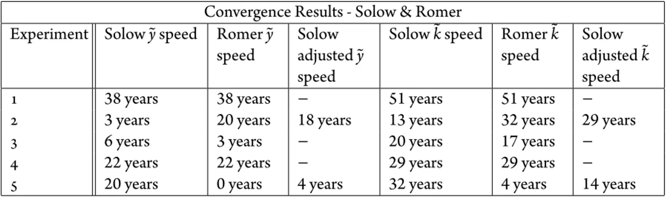
In other words, we must find the particular time t at which the values of ˜y and ˜k satisfy the above inequalities. The results of convergence are presented in Table 3.4 below.
A remark: In experiments 2 and 5, the technological growth rate gAwithin the Romer model was not invariant. Hence, in order to have a ”fair” comparison, I also changed the tech-nological growth rates g in period t= 5 within the Solow model in experiments 2 and 5 to the ones given by the Romer model for the purposes of analyzing the speed of convergence. These adjustments are listed in Table 3.4 as ”Solow adjusted ˜y speed” and ”Solow adjusted ˜k speed”. ”Solow ˜y speed” and ”Solow ˜k speed” refer to the instances in which the technology growth rate g in the Solow model has not been changed during period t= 5.
From Table 3.4 we can conclude that within both models, capital per effective worker ˜k takes longer to converge to the new steady-state than output per effective worker ˜y. In exper-iments 1 and 4, the speed of convergence is equal within both models. During experiment 3, the Romer economy converged faster to the new steady-state by 3 years. In experiments 2 and 5, where the technological growth rate gAof the Romer model is not invariant, there
ex-Convergence Results - Solow & Romer Experiment Solow ˜y speed Romer ˜y
speed
Solow adjusted ˜y speed
Solow ˜k speed Romer ˜k speed
Solow adjusted ˜k speed
1 38 years 38 years − 51 years 51 years −
2 3 years 20 years 18 years 13 years 32 years 29 years
3 6 years 3 years − 20 years 17 years −
4 22 years 22 years − 29 years 29 years −
5 20 years 0 years 4 years 32 years 4 years 14 years
Table 3.4:Convergence Results.
ists large differences between the two convergence speeds. The Romer model converges slower in experiment 2 and in experiment 5 the Romer model converges faster than the Solow model - by a substantial amount in both cases. However, if one adjusts the techno-logical growth rate g within the Solow model with that of the Romer model, then the speeds of convergence are fairly close within both models.
Alles ist einfacher, als man denken kann, und zugleich verschränkter, als zu begreifen ist.
Translated from German into English:
Everything is simpler than you think and at the same time more complex than you imagine.
Johann Wolfgang von Goethe
4
Conclusion
T
he conclusion of the prior investigation is summarized in the following. The exper-iments have served their purpose in fulfilling the aims which were set in the introduction section of Chapter 0, that is, they have indicated how the two models can be used to analyze different economic scenarios.In particular, experiment 1 shows the implications of an increase of the saving rate. As the simulation and the mathematical equations show, this results in an increase in both output and capital per effective worker in both models.
The second experiment investigated the scenario of a decrease in the population growth rate. The results of a decrease in the population growth rate produced a higher output per effective worker and capital per effective worker in both, the Solow and the Romer economy. Furthermore, the experiment showed that such a decrease also results in a decrease of the technological rate and the share of the population which is engaged in research. This result was showcased by the Romer model, whereas the Solow model suffers from the incapabil-ity to explain the nature of the technological growth rate. Thus, the technological growth rate and the share of the population engaged in research are not invariant to a change in the population growth rate.
Experiment 3 showed that a decrease in the output elasticity of capital will decrease the steady-state values in both models and additionally, the Romer model suggests that such a decrease will unavoidably decrease the share of the population which is engaged in research.
The fourth experiment illustrated the case of the change in the depreciation rate. An in-crease leads to the dein-crease of the steady-state values of output and capital per effective worker and a decrease will increase them. Furthermore, the technology growth rate and the share of the population engaged in research remain invariant to the change in the depreci-ation rate.
Lastly, the final and fifth experiment investigated the increase in the population and saving rates simultaneously. This implied that when changing two opposing forces within a model it has to be precautioned by which amount these variables are changed in order for a positive result to occur.
Furthermore, this report, in particular Chapter 3, summarizes the necessary restrictions - using real world data - which a simulator utilizing the Solow and Romer models should
set. That is, the values of the output elasticity of capital, the population growth rate, the sav-ing rate, the growth rate of technology, the depreciation rate, the parameters of the Romer model, and also briefly discusses the realistic choices for the discount rate and the share of the population which is engaged in research and development. This in particular answers one of the questions raised in the problematization section of Chapter 0, ”Which values for the parameters are ’reasonable’ choices?”.
Another problem which was layed out in the problematization section of Chapter 0 was that of the speed of convergence. Chapter 3 section ”The Speed Of Convergence” provides a method for analyzing such problems. In experiments 1 and 4 the models converged at the same speed. In experiment 3, the Romer economy converged faster to the new steady-state by a small amount. Within experiments 2 and 5, where the technological growth rate was not invariant, there was a substantial difference between the two models. The Romer model converged slower by a substantial amount in experiment 2 and faster in experiment 5. However, if the growth rate of technology within the Solow model was adjusted, then both models converged almost at the same speed.
What remains to be answered is the final question raised in Chapter 0: ”Which model is more adequate for the purpose of analyzing different economic scenarios using a
simu-lated environment?”. The answer is that both models have the necessary capabilities for such an undertaking. However, if one desires to know the impact and the nature of technologi-cal growth, then the Romer model is better suited for the problem at hand since the Solow model is ill-suited for such an investigation. Additionally, the Romer model can give insights into the implications of the share of the population which is engaged in research. On the other hand, if the technological progress may be treated as exogenous, then the Solow model might be the better tool for the problem at hand given its simplistic nature. In short, one should use the right tool for the right job.
To summarize, this paper showed that both models can be used for the investigation of different economic scenarios and it gathers the necessary restrictions for the input variables to the models. Furthermore, Chapter 3 provides a mathematical method for analyzing the speed of convergence. The simulations confirm whatSolow(1956) proposed: That tech-nological growth is one of the key factors for economic growth. Furthermore, this report illustrated the defficiencies of the Solow economy and showcased the benefits of the more modernRomer(1990) model, which indicates that the next logical step was to endogenize the growth rate of technology, although its introduction into economic growth theory had to be postponed as explained byRomer(1994).
Further Investigations
Given that this paper simulates the economic scenarios only on a partial transition dynamics, it does not capture the entire phenomenon of economic growth. An interesting aspect which is not included is that of the complete transition dynamics from one steady-state to the other as used within theRomer(1990) andJones(1995) papers. An investigation into the simu-lation of the transition dynamics - especially that of the Romer model - is an interesting and possibly fruitful pursuit which one may consider.
Lastly, it is argued and partial evidence suggests that the population does not grow expo-nentially at every point in time as assumed in the Solow and Romer models (Mulligan,2006). There exists a second model for population growth called logistic population growth. In this model, the population grows exponentially until a certain period of time and reaches a point of change, where the population growth does not grow exponentially anymore and starts to grow at a slower rate until it reaches some certain upper bound - a supremum to be precise
- which could possibly indicate the Earth’s maximum capacity to provide humans with land and other natural resources. An intriguing investigation following this discussion is to modify the assumptions of growth models which assume exponential population growth to the logis-tic growth model and simulate such scenarios. Such analysis would indicate the interaction between different fields, such as economics and demography.
References
Apostol, T. M. (1969). Calculus, Volume II: Multi-Variable Calculus and Linear Algebra, with
Applications to Differential Equations and Probability, volume Vol. 2. John Wiley and Sons, 2
edition.
Besomi, D. (2001). Harrod’s dynamics and the theory of growth: the story of a mistaken attribution. Cambridge Journal of Economics, 25(1), 79–96.
Blume, L. E. & Sargent, T. J. (2015). Harrod 1939. The Economic Journal, 125(583), 350– 377.
Cobb, C. W. & Douglas, P. H. (1928). A theory of production. The American Economic
Review, 18(1), 139–165.
Friedberg, S. H., Insel, A. J., & Spence, L. E. (1979). Linear Algebra. Englewood Cliffs, N.J.: Prentice-Hall, 1 edition.
Halsmayer, V. & Hoover, K. D. (2016). Solow’s harrod: Transforming macroeconomic dynamics into a model of long-run growth. The European Journal of the History of Economic
Thought, 23(4), 561–596.
Harrod, R. F. (1939). An essay in dynamic theory. The Economic Journal, 49(193), 14–33. Inada, K.-I. (1963). On a two-sector model of economic growth: Comments and a general-ization. The Review of Economic Studies, 30(2), 119–127.
Jones, C. I. (1995). R & d-based models of economic growth. Journal of Political Economy, 103(4), 759–784.
Jones, C. I. & Vollrath, D. (2013). Introduction to Economic Growth. W. W. Norton and Co., 3 edition.
Li, H. & Zhang, J. (2006). How effective is the one-child policy in china? Working Paper