PINT: a software for integration of peak volumes and extraction of relaxation rates

PINT: a software for integration of peak

volumes and extraction of relaxation rates

Alexandra Ahlner, Mats Carlsson, Bengt-Harald Jonsson and Patrik Lundström

Linköping University Post Print

N.B.: When citing this work, cite the original article.

The original publication is available at www.springerlink.com:

Alexandra Ahlner, Mats Carlsson, Bengt-Harald Jonsson and Patrik Lundström, PINT: a software for integration of peak volumes and extraction of relaxation rates, 2013, Journal of Biomolecular NMR, (56), 3, 191-202.

http://dx.doi.org/10.1007/s10858-013-9737-7

Copyright: Springer Verlag (Germany)

http://www.springerlink.com/?MUD=MP

Postprint available at: Linköping University Electronic Press

1

PINT – a Software for Integration of Peak Volumes and Extraction of

Relaxation Rates

Alexandra Ahlner, Mats Carlsson, Bengt-Harald Jonsson and Patrik Lundström*

Division of Molecular Biotechnology Department of Physics, Chemistry and Biology

Linköping University SE-58183 Linköping, Sweden

2

Abstract

We present the software PINT (Peak INTegration), designed to perform integration of peaks in NMR spectra. The program is very simple to run, yet powerful enough to handle complicated spectra. Peaks are integrated by fitting predefined line shapes to experimental data and the fitting can be customized to deal with, for instance, heavily overlapped peaks. The results can be inspected visually, which facilitates systematic optimization of the line shape fitting. Finally, integrated peak volumes can be used to extract parameters such as relaxation rates and information about low populated states. The utility of PINT is demonstrated by applications to the 59 residue SH3 domain of the yeast protein Abp1p and the 289 residue kinase domain of murine EphB2.

3

Introduction

The results of many areas within the field of NMR spectroscopy depend on correctly estimated peak volumes in the NMR spectra. One area where this is particularly important is characterization of protein dynamics. The simplest way of estimating peak volumes is to approximate them with their corresponding intensities. While this method is simple and works well for non-overlapped peaks it has drawbacks even under this assumption. One is that experimental noise is not averaged so that the uncertainty in the peak volume will be unnecessarily large, especially for spectra with low signal to noise ratios. A slightly better method is thus to estimate the volume as the average intensity of several points around the peak maximum, which for instance is used in the seriesTab protocol in the NMRpipe suite (Delaglio et al. 1995). Experimental noise that varies on a point-to-point basis is thus averaged and improved accuracy may be obtained. This method is however equally poorly suited for dealing with overlapped peaks. To be able to handle this case and to use all information the peak contains, the method of choice is to fit the peak to a functional form that represents its line shape or in the case of overlapped peaks to a sum of such functions. This involves optimizing the parameters chemical shifts, line widths and intensity at peak maximum by minimizing the sum of squared residuals between the experimental data and the fitted line shape. The peak volume is then estimated as the volume of the fitted line shape, which is trivial to calculate.

There already exist several excellent programs for this purpose (Delaglio et al. 1995; Goddard and Kneller ; Koradi et al. 1998; Korzhnev et al. 2001; Romano et al. 2008) but we have been increasingly convinced that their use often is omitted in favor of the more simplistic and limited approaches described above. We speculate that the reason for this is that many of them are too complicated for the average user, that they impose too strict demands on the format of input data or that they lack functionality so that a myriad of other programs and scripts must be used for simple downstream tasks such as extraction of relaxation rates.

With this in mind we wrote the program PINT (Peak INTegration). PINT is written in C++ and is available for a variety of Linux distributions and Mac (Darwin). PINT integrates peaks in two-dimensional or pseudo three-dimensional spectra processed with NMRpipe, using a peak list in almost any format, in a fashion that depends on instructions given in a

4 user-written parameter file. The minimal parameter file simply comprises two lines specifying which spectrum to integrate and which peak list to use but many more options are available either to improve the quality of the integration if necessary or to incorporate downstream tasks. After peak integration has been performed, the agreement between experimental data and fitted line shapes can be inspected in the freeware Gnuplot (Williams and Kelley 2010). It is thus easy to identify problematic peaks, for which the fit either did not converge or converged to the wrong result, and customize the parameter file in a systematic fashion to improve the result. Another feature of PINT is that the uncertainty in the estimated volumes is automatically calculated if duplicate data points have been recorded. Although PINT was coded from scratch, it is heavily influenced by FuDA (http://pound.med.utoronto.ca/~flemming/fuda/) that includes many of the features that are found in PINT and is used in a similar way.

The primary output of PINT is one file for every peak in the peak list with volumes and associated uncertainties as a function of an index or a user supplied arrayed parameter. It also includes information about the fitted peak position and line width in the two dimensions and details of the fit.

We exemplify peak integration and extraction of relaxation rates using two different proteins of various sizes, resulting in spectra of different complexity. The first protein used is an SH3 domain from the yeast protein Abp1p (Drubin et al. 1990; Lila and Drubin 1997; Rath and Davidson 2000) comprising 59 residues and the second protein is the kinase domain from murine EphB2 (Gale et al. 1996) that consists of 289 residues (Figure 1).

5

Figure 1. A) 15_N-1_{H HSQC correlation map of an SH3 domain from the yeast protein Abp1p, comprising 59}

residues. B) 15_N-1_{H TROSY correlation map of the kinase domain of murine EphB2, comprising 289 residues.}

The protein has the following mutations: Ser677Ala, Ser680Ala, Asp754Ala. Both data sets were collected at 600 MHz.

Results and Discussion

PINT calculates the volumes of peaks in two-dimensional NMR spectra by performing a non-linear least-square fit (Press et al. 1988) of the experimental data to a specific line shape, by optimizing peak positions, line widths and intensity. Formally, PINT minimizes the target function 𝜒2 _{= � � �}𝑓(𝑥𝑖, 𝑦𝑖, 𝐼𝑗, 𝑥0, 𝑦0, Δ𝑥, Δ𝑦) − 𝐼𝑗(𝑥𝑖, 𝑦𝑖) 𝜎 � 2 𝑖 𝑗 (1)

where 𝐼𝑗(𝑥𝑖, 𝑦𝑖) is the intensity at (𝑥𝑖, 𝑦𝑖), 𝜎 is the spectral noise, 𝑓(𝑥𝑖, 𝑦𝑖, 𝐼𝑗, 𝑥0, 𝑦0, Δ𝑥, Δ𝑦) is

the fitted line shape with the adjustable parameters 𝐼𝑗, which is the intensity at peak

maximum, 𝑥0 and 𝑦0 that are the fitted positions of the peak maximum and Δ𝑥 and Δ𝑦 that

are the line widths in the two dimensions. For one of the implemented line shapes there are two additional adjustable parameters (see below). The summation i runs over all points that define the peak and the summation j runs over all spectra that are integrated, which means that the optimized peak positions and line widths are the same for all spectra. For example, if 15 spectra are integrated, there are 19 (21 for one of the line shapes) optimized parameters, corresponding to the 15 peak intensities and peak positions and line width in the two dimensions, for each peak. In what follows we use italic font for PINT options, surround arguments to the options with angle brackets and capitalize reserved words. Peak integration by PINT is performed using the command

6 The parameter file contains instructions on how to perform the line shape fitting. The results are written to the output directory and files generated to allow a visual inspection of the integration are written to the plot directory. PINT neither creates these directories nor removes their contents after a previous run. Hence, the user must perform this, either manually or by running PINT from a shell-script that automates these tasks. A typical PINT session comprises the following steps:

1. Write a minimal parameter file. 2. Run PINT to integrate the peaks.

3. Inspect the results visually using Gnuplot.

4. Modify the parameter file to improve integration of problematic peaks. 5. Repeat from step 2 until all peaks are successfully integrated.

6. Modify the parameter file to incorporate extraction of relaxation rates or other downstream tasks if desired.

The PINT parameter file

The integration is regulated by different options in the PINT parameter file. The minimal parameter file only comprises the following two lines

-spectrum <name of spectrum> -peakList <name of peak list>

PINT uses this information to integrate the peaks specified by the peak list in the specified spectrum by fitting a gaussian line shape to a default-sized region of the spectrum surrounding all peaks with chemical shifts defined in the peak list. The spectrum and the peak list may be located in an arbitrary directory as long as the correct path is specified.

The spectrum must be a two-dimensional or pseudo three-dimensional spectrum in NMRpipe format (Delaglio et al. 1995). In the latter case, it should be represented as a cube, not as a collection of files corresponding to the various planes. It is however also possible to integrate several different two-dimensional spectra, corresponding to different planes of a

7 pseudo three-dimensional spectrum, using a slightly different syntax. To do this the minimal parameter file is instead

-spectrumList <name of spectrum list> -peakList <name of peak list>

where the spectrum list is a file that contains lines with the name of each spectrum to integrate. Note that the peak list is common for all spectra in this case.

The peak list defines the chemical shifts and the assignments for the peaks to fit. An example of an allowed peak list is shown in Figure 2.

Figure 2. Example of a peak list that can be used by PINT. If the order of the columns differs from default, i.e.

assignment in column 1, chemical shift in the indirect dimension in column 2 and chemical shift in the direct dimensions in column 3, the actual order of columns may be specified and it is perfectly fine to use peak lists with more than three columns. In the example above, the first line is a header. The flag –skipLines <n> can be used to disregard from the n leading lines in a peak list.

The peak list must contain at least three columns corresponding to assignment and peak position in the indirect and direct dimensions. All assignments must be unique and any characters except a slash (/) are allowed in assignments. Empty lines and lines starting with a pound sign (#) are ignored and there is no limit on the allowed number of lines in the peak list. PINT is very flexible regarding the format of the peak list as described in the

8 legend to Figure 2. Peaks may be folded an arbitrary number of times but partially folded peaks are not allowed.

Visual inspection of the quality of the line shape fitting

A useful way to evaluate the quality of the fit or reasons for non-convergence is to visually inspect how well the fitted line shape agrees with the experimental data. Plot files are therefore created regardless of whether the fitting converged or not. For every fitted peak and plane in the spectrum, the files assi_001.dat, assi_002.dat… assi_n.dat, where assi is the assignment, are created. The files contain intensities for the experimental data and for the fitted line shape as a function of the coordinates for the various planes of the pseudo three-dimensional spectrum or list of two three-dimensional spectra. PINT also creates the Gnuplot input files assi.gnu that lets the user browse through the planes for each peak and the file plotfits.gnu where all peaks can be inspected at once. Gnuplot (Williams and Kelley 2010) is a freeware for Linux and Mac. To browse through peaks, go to the directory where the plot files are written and type gnuplot plotfits.gnu on the command line.

Since the intensity is the only parameter that differs for a given peak between planes, browsing through all of them for all peaks can be very time consuming and often unnecessary. To select only one of the planes to plot one can thus use the option -plane2plot <selected plane> to only write a selected plane to the plotfits.gnu file to speed up the process. Data for all planes are however always written to the files assi.gnu so all planes for a particular residue can always be viewed. It is usually easy to get an idea if the fit is satisfactory or not as well as the underlying reason for this, as can be seen in Figure 3.

9

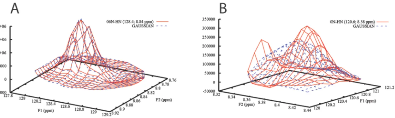
Figure 3. A) Satisfactory integration of peak 06N-HN and B) failed integration of peak 0N-HN from SH3

domain of Abp1p plotted with Gnuplot. The experimental data is represented as solid red lines and the fitted line shapes as dashed blue lines. The failure in the latter case is due to the presence of a nearby intense peak. Possible remedies in this and similar cases are described below (c.f. Figure 5).

Improving integration

For most peaks in a typical spectrum, default parameters provide satisfactory results. For problematic peaks we provide customizing options. Some are described herein and the remainder in the file README.txt that comes with the distribution.

Customizing line shape and area of integration

If for example the gaussian line shape does not fit the peaks well, the lorentzian function and function corresponding to a weighted sum of gaussian and lorentzian functions (GALORE) are also implemented. Among the different ways of implementing a weighted sum of lorentzian and gaussian line shapes, we opted for

𝑓�𝑥, 𝑦, 𝐼𝑗, 𝑥0, 𝑦0, Δ𝑥, Δ𝑦, 𝑤𝑥, 𝑤𝑦�

= 𝐼𝑗⋅ �𝑤x⋅ lx(𝑥, 𝑥0, Δ𝑥) + (1 − 𝑤𝑥) ⋅ gx(𝑥, 𝑥0, Δ𝑥)�

⋅ �𝑤𝑦⋅ ly�𝑦, 𝑦0, Δy� + (1 − 𝑤𝑦) ⋅ gy(𝑦, 𝑦0, Δ𝑦)�

(2)

where lx, ly, gx and gy are one-dimensional lorentzian and gaussian line shapes normalized

10 and the other symbols have the same meaning as in Equation 1. To change the line shape, append the line

-lineShape <line shape>

where the argument can take the values GAUSSIAN, LORENTZIAN or GALORE to the parameter file. Quite often, all three line shapes fit the data reasonably well and as expected the GALORE line shape usually fits the data best at the expense of the two extra fitting parameters.

Sometimes only a subset of the peaks benefit from another line shape than specified by global settings. In this case, you append the line

-defineLineShape <assi> < line shape>

to change the line shape for a peak with assignment assi. Great caution is necessary when comparing volumes of peaks integrated with different line shapes.

In fact, all PINT options are possible to customize on a peak-by-peak basis using the same syntax. Thus, to change the area that is considered for integration globally you append -radius <radius in F1 (ppm)> <radius in F2 (ppm)> and to do the same for a selected peak you append -defineRadius <assi> <radius in F1 (ppm)> <radius in F2 (ppm)> to the parameter file. This is useful for spectra where the default radii, do not cover enough of the peak or covers unnecessarily large areas. We have elected to use units of ppm for all spectrum related user input since it is the normal units in NMR spectra. Accordingly, if the user wants to customize the guessed line width for the line shape fitting to improve the rate of convergence also these are entered in ppm, i.e. -lineWidth <guessed line width in F1 (ppm)> <guessed line width in F2 (ppm)>.

The convergence criterion is that the change in χ2_{, defined as above, between}

successive iterations is less than a value that the user may customize. Another parameter that is of some relevance for convergence is the uncertainty in the data points, i.e. σ in Equation 1, is specified as

11 -noise <noise>

Correctly estimated noise is obviously crucial for calculating the ‘correct’ χ2_{. Note that a}

common noise level is used for all spectra if several spectra are integrated. All different ways to customize the fit are described in the file README.txt.

Overlapped peaks

For a group of overlapped peaks, simultaneous integration of all peaks in the group is crucial. By simultaneous integration, we mean that the target function to minimize for this group of peaks is 𝜒2 _{= � � � �}𝑓𝑘(𝑥𝑖, 𝑦𝑖, 𝐼𝑗𝑘, 𝑥0𝑘, 𝑦0𝑘, Δ𝑥𝑘, Δ𝑦𝑘) − 𝐼(𝑥𝑖, 𝑦𝑖) 𝜎 � 2 𝑖 𝑗 𝑘 (3)

where k is an index that runs over all peaks in the group and the other parameters are defined as in Equation 1. To integrate peaks with assignments assi1 and assi2 as a group, the following line is added to the parameter file

-overlap <assi1> <assi2>

There is no restriction of number of peaks in an overlapped group. In practice, it is limited by computational power. Similarly, there is no restriction in the number of groups with overlapped peaks. Figure 4 shows peak 39N-HN of an SH3 domain of the protein Abp1p that is heavily overlapped with peak 48N-HN fitted without and with considering overlap. The improvement when the two peaks are fitted as a group is obvious. The figure also shows successful integration of two groups of four overlapped peaks each in the kinase domain of murine EphB2.

12 overlapped it is also possible to let PINT decide which ones that are based on their chemical shifts and the specified areas for integration. To do this, add the line -overlap auto to the parameter file. The automated mode of determining peak overlap also results in a file, with lines of the format -overlap <assignment 1> <assignment 2> … for every overlapped group, that may be modified and pasted into the parameter file if the user is not content with the automated mode.

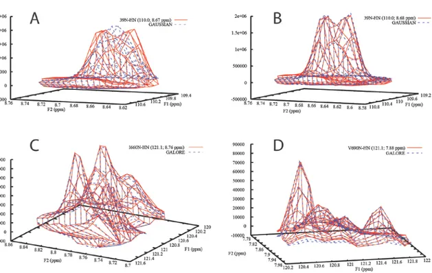
Figure 4. Peak 39N-HN of the SH3 domain of Abp1p first integrated with A) global settings and then B)

improved by integration together with overlapped peak 48N-HN. C-D) Two integrated groups of four peaks from the kinase domain of murine EphB2. The experimental data is plotted as solid red lines and the fitted line shapes as dashed blue lines.

Another way of dealing with partially overlapped peaks is to reduce the area considered for integration for a subset of the peaks to reduce the influence of nearby peaks as described above. This flag can be used either alone or in combination with the –overlap flag. Similar results can often be achieved by reducing the area of integration and integrating the peak as

13 an overlapped group as shown in Figure 5. Hence, this flag is particularly useful for reducing the number of peaks that have to be included in an overlapped group and thereby speed up the integration.

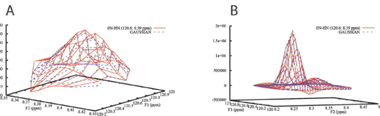
Figure 5. Peak 0N-HN of the SH3 domain of Abp1p integrated A) with a reduced radius of the integration area

and B) as part of an overlapped group. The experimental data is plotted as solid red lines and the fitted line shapes as dashed blue lines. The volumes of peak 0N-HN are 7000±50 and 7400±90 in A and B, respectively. Note that 0N-HN is the minor peak in B.

Error estimation

Correct estimation of uncertainties in peak volumes is important but not straightforward. A common method is to use one or two duplicated data points and estimate the error as the absolute value of the difference between the duplicate points. This is a notoriously unreliable method since the duplicate points may overestimate or underestimate the error by chance and instead often an ad hoc minimal error has to be specified. The use of duplicate measurements should thus only be used if a sufficiently large number of duplicate points have been recorded so that the statistics is reliable. We supply two options for estimating uncertainties in peak volumes. The default method is based on the assumption that the distribution of difference in volumes for duplicate points is the same for all peaks and one common value for the uncertainty is thus calculated for all peaks. In practice, this requires that the volumes of all peaks are similar so this approach will not give correct uncertainties for peak volumes that are much larger or smaller than average. In the other method, designed to handle this case, a unique value of the uncertainty is calculated for each peak. It is also possible to use a hybrid method, i.e. estimate the error globally for most

14 residues except for selected ones.

Result of peak integration

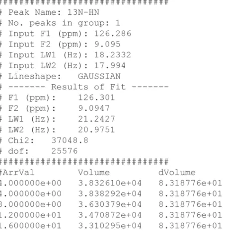
After the fit is completed, the result is presented in various output files. Some are always produced but others are only created optionally or to indicate failure. For each peak with a converged fit, the file assi.out, where assi is the assignment, is generated. An example of such a file is shown in Figure 6. The first part of the file contains input information such as the assignment, input peak position, input line width, number of peaks integrated together and line shape. The result of the fit is thereafter presented as the fitted peak position and line widths in both dimensions. The parameter χ2, which is the sum of the squared residuals

from the fit, is also presented together with degrees of freedom. The file ends with the peak volume(s), and if duplicate experiments have been recorded their uncertainties as a function of an index or an arrayed parameter (c.f.). No attempt is made to calculate uncertainties unless duplicate experiments have been performed. Peaks with non-converged fits are listed in the file error.txt together with error messages.

15

Figure 6. Illustration of a PINT output file. The file is divided into three parts. The first part contains input

parameters and options for the integration, the second part contains the results of the fit and the third part consists of the fitted volumes as a function of an arrayed parameter or an index. Arrval is the value of the arrayed parameter, Volume is the fitted peak volume and dVolume is its uncertainty.

Downstream analysis

One of the features with PINT is the built-in conversion of peak volumes to quantities such as relaxation rates, hydrogen exchange rates or the heteronuclear NOE. Our intention is that evaluating data will become easier when the entire procedure is contained in the same program. Since common chemical shifts and line widths are fitted for all spectra, multiple runs of PINT are however required for applications such as titrations and studies of protein-protein interactions. The implemented curve-fitting routines and calculations to extract relaxation rates and other parameters from the integrated peak volumes are summarized in Table 1.

16

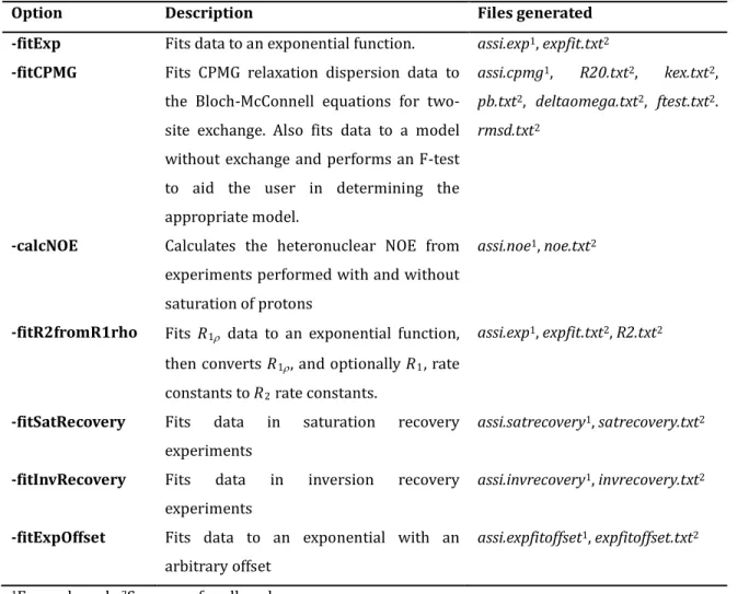
Table 1. Implemented types of downstream analysis

Option Description Files generated

-fitExp Fits data to an exponential function. assi.exp1_{, expfit.txt}2 -fitCPMG Fits CPMG relaxation dispersion data to

the Bloch-McConnell equations for two- site exchange. Also fits data to a model without exchange and performs an F-test to aid the user in determining the appropriate model.

assi.cpmg1_{, R20.txt}2_{, kex.txt}2_,

pb.txt2_{, deltaomega.txt}2_{, ftest.txt}2_.

rmsd.txt2

-calcNOE Calculates the heteronuclear NOE from experiments performed with and without saturation of protons

assi.noe1_{, noe.txt}2

-fitR2fromR1rho Fits R1ρ data to an exponential function, then converts R1ρ, and optionally R1, rate

constants to R2 rate constants.

assi.exp1_{, expfit.txt}2_{, R2.txt}2

-fitSatRecovery Fits data in saturation recovery experiments

assi.satrecovery1_{, satrecovery.txt}2 -fitInvRecovery Fits data in inversion recovery

experiments

assi.invrecovery1_{, invrecovery.txt}2 -fitExpOffset Fits data to an exponential with an

arbitrary offset

assi.expfitoffset1_{, expfitoffset.txt}2 1_{For each peak,} 2_{Summary for all peaks}

To use these routines, the values of the arrayed parameter must be specified. This is done by the flag

-arrVal <value 1> <value 2> …

Varian (Agilent) users have the option of instead retrieving the values of the arrayed parameter from the procpar file by using the flags

-procpar <path to procpar file> -array <name of arrayed parameter>

17 Errors in the model parameters are estimated with the jackknife method (Mosteller and Tukey 1977), which is robust for data sets comprising more than a few data points and has the added advantage over Monte Carlo simulations or estimations from the covariance matrix that the estimated errors are less dependent on the uncertainty in the individual data points.

Analysis of fast dynamics

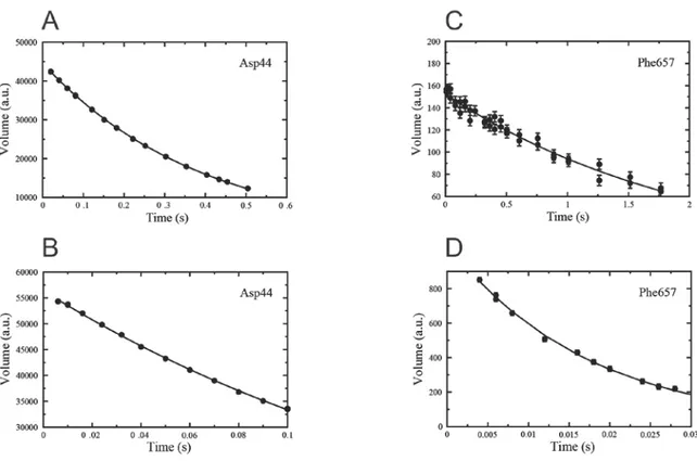
The decaying exponential is probably the most common function to fit NMR data to and applications include extraction of relaxation rates and hydrogen exchange rates (Dempsey 2001). PINT fits exponentially decaying data if the flag –fitExp is used. For each residue, an output file called assi.exp is generated. It contains the data of the exponential fit in the form of the volume at time zero, the decay constant and their uncertainty estimated with the jackknife method. The ending part of the file contains the time, the fitted volume, the estimated error in the volume and the volume calculated from the exponential fit. The estimated errors are only present when duplicated experiments have been performed. Figure 7 shows the exponential fit of R1 data for peak Asp44 of an SH3 domain from Abp1p

and Phe657 of the kinase domain from EphB2. The model parameters and associated uncertainties for all peaks are summarized in the file expfit.txt.

18

Figure 7. The results of an exponential fit. 15_{N A) R1 and B) R1ρ relaxation rates for residue Asp44 of an SH3}

domain from the yeast protein Abp1p. The extracted rate constants are 2.57 ± 0.01 s-1 _{and 5.25 ± 0.05 s}-1_,

respectively. 15_{N C) R1 and D) R1ρ relaxation rates for residue Phe657 of the kinase domain of murine EphB2.}

The extracted rate constants are 0.48 ± 0.02 s-1 _{and 58 ± 1 s}-1_{, respectively. Filled circles and error bars}

represent peak volumes with associated uncertainties and the solid lines represent the best fit to exponential functions. Both data sets were recorded at 600 MHz. The figure was prepared with Grace (Stambulchik 1998) using unmodified PINT output files.

We also provide a routine for calculating the heteronuclear NOE, -calcNOE, so that PINT can take care of the entire process of generating model-free (Clore et al. 1990; Lipari and Szabo 1982a; Lipari and Szabo 1982b) input from a set of spectra, corresponding to measurements of R1, R2 and NOE. Since the common method of recording NOE is to simply

record duplicates of experiments with or without presaturation of the protons, our usual method of estimating uncertainties in peak volumes fails. Thus, the uncertainty in the NOE is reported as the standard error of all permutations of the ratio of experiments with and without presaturation of the protons.

19 It is common to measure R1ρ rather than R2. To fit R1ρ relaxation rates and convert

these to R2 rates one can use the following syntax in the parameter file

-fitR2fromR1rho

-b1 <spinlock field strength (Hz)> -carrier <carrier position (ppm)>

-r1List R1.txt <List with R1 rate constants>

This will perform an exponential fit to extract R1ρ values and thereafter calculation of R2

from R1ρ and R1 using the following equation

𝑅2 = 𝑅1ρ⁄sin2θ − 𝑅1/ tan2θ (4)

where θ is the tilt-angle, defined as tan θ = B1/Ω, B1 and Ω are the spinlock field strength and

the offset from the carrier, respectively, and R₁ is the longitudinal relaxation rate.

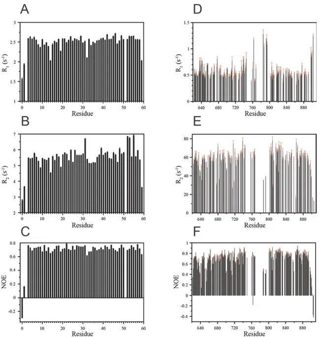
Figure 8 shows results of determination of 15_{N R1, R2 rates and the {}1_H}-15_N

heteronuclear NOE for an SH3 domain from Abp1p and for the kinase domain from EphB2, where the input files for the plots are generated by PINT.

20

Figure 8. 15_{N R1 and R2 relaxation rates and the {}1_H}-15_{N heteronuclear NOE for A-C) an SH3 domain from the}

yeast protein Abp1p and D-F) the kinase domain of EphB2. All data was recorded at 600 MHz, fitted with PINT and plotted with Grace (Stambulchik 1998) using unmodified PINT output files. For clarity, the error bars in D-F are colored red. Note that the relaxation rates for the kinase domain of EphB2 indicates that it forms homodimers in solution.

A number of common NMR experiments result in data that does not decay exponentially to zero but to a plateau. Examples are inversion recovery, saturation recovery and certain amide proton exchange experiments. We provide three different routines for

21 this. The options -fitInvRecovery and -fitSatRecovery fit data to the equations I = I0[1 − 2 exp(−R ⋅ t)] and I = I0[1 − exp(−R ⋅ t)], respectively, while a three parameter fit,

i.e. I = I0exp(−R ⋅ t) + A, is performed using the option -fitExpOffset. We point out that it is

permitted to perform fits to more than one model in a single run of PINT. This is useful if it is not known a priori which of several models that fits the data better.

Analysis of Carr-Purcell-Meiboom-Gill relaxation dispersion

The Carr-Purcell-Meiboom-Gill (Carr and Purcell 1954; Meiboom and Gill 1958) relaxation dispersion experiment is extremely powerful for characterizing millisecond molecular dynamics in terms of exchange rates, populations and chemical shift differences between exchanging states (Mittermaier and Kay 2006). In these experiments the effective transverse relaxation rate is monitored as a function of the repetition rate of 180° refocusing pulses (Hansen et al. 2008; Loria et al. 1999; Mulder et al. 2001). PINT fits these effective transverse relaxation rates to the Bloch-McConnell equations (McConnell 1958) including or excluding two-state chemical exchange. An F-test is performed so that the user can select the appropriate model. The arrayed parameter in this case is half the number of 180° refocusing pulses, ncyc, during a relaxation delay of duration 𝑇. PINT first converts it to the repetition rate 𝜈𝐶𝐶𝐶𝐶 = 𝑛𝑛𝑦𝑛/𝑇, and the peak volumes to effective transverse

relaxation rates

𝑅2,𝑒𝑒𝑒(𝜈𝐶𝐶𝐶𝐶) =ln �𝐼0/𝐼(𝜈_𝑇𝐶𝐶𝐶𝐶)� (5)

where I0 and 𝐼(𝜈_{𝐶𝐶𝐶𝐶}) are the peak volumes in the absence and presence of the constant

time relaxation delay, respectively. To fit CPMG data acquired with a constant time relaxation delay of T seconds, add the lines

–fitCPMG –time_T2 <T>

22 For a peak with assignment assi, the results of the CPMG fits are presented in the file assi.cpmg. The first part of this file resembles assi.out, but in addition, it contains the extracted parameters of the CPMG fit as well as the experimental and fitted 𝑅2,𝑒𝑒𝑒 as a

function of 𝜈𝐶𝐶𝐶𝐶. Files that summarize the extracted parameters for all residues as well as

the results of the F-tests are also generated.

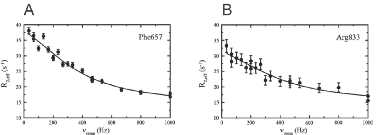
Figure 9. The results of the analysis of A) Phe657 and B) Arg833 of the kinase domain of EphB2 15_{N CPMG}

relaxation dispersions. The calculated values of R2,eff are plotted against νCPMG, with the error estimated from

duplicate experiments and the fitted R2,eff plotted as a line. The exchange parameters are R2,0 = 33 ± 3 s-1, kex =

2400 ± 200 s-1_{, pB = 13 ± 9%, ∆ϖ = 0.14 ± 0.03 ppm for Phe657 and R2,0 = 33 ± 3 s}-1_{, kex = 2700 ± 700 s}-1_{, pB =}

15 ± 5%, ∆ϖ = 0.12 ± 0.01 ppm. The data was recorded at 800 MHz. The figure was prepared with Grace (Stambulchik 1998) using unmodified PINT output files.

Examples of fitted CPMG relaxation dispersion profiles are shown in Figure 9. We emphasize that off-resonance effects and pulse imperfections are not taken into account and that exchange rates and populations are fitted on a peak-by-peak basis. For more rigorous and flexible fitting we refer the user to specialized software such as CATIA (http://pound.med.utoronto.ca/~flemming/catia/).

Performance

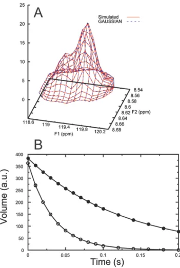
To demonstrate that PINT can calculate accurate volumes and relaxation rates we integrated a synthetic data set comprising 15 planes of a pseudo three-dimensional spectrum containing 58 gaussian shaped peaks with added pseudo-random noise, including seven

23 groups with two overlapped peaks and one group with three overlapped peaks. The different planes represented relaxation delays and the intensities of the peaks were scaled to decay exponentially. For the two peaks in one of the overlapped groups the decay rates were set to 8 s-1 _{and 30 s}-1_{, respectively, and for the remainder of the peaks they were set to}

12 s-1_{. The integrated peak volumes were fitted to an exponential function in PINT.}

Regardless of which seed that was used for the random number generator the average fitted decay rate for the peaks with uniform rate constants was 12.00 ± 0.01 s-1_{. The fitted rate}

constants for the two overlapped peaks with different rate constants were also distributed narrowly around the preset decay rates for different choices of seed for the random number generator. A typical example is shown in Figure 10. The average relaxation rates for twenty simulations using different random seeds were 8.00 ± 0.02 s-1 _{and 30.0 ± 0.1 s}-1_,

respectively.

24 spectrum was generated by calculating gaussian functions with pseudo-random noise. The peaks were assigned decay rates of 8 s-1 and 30 s-1, respectively and 15 spectra corresponding to different relaxation delays were generated. A) Data (red solid lines) and the fitted line shapes (blue dashed lines) for a spectrum corresponding to a relaxation delay of 20 ms. B) Integrated peak volumes (filled and open circles) as a function of the relaxation delay and fits to exponential functions (lines). The fitted decay rates are 7.99 ± 0.02 s-1 _{and 29.9 ± 0.1 s}-1_{, respectively.}

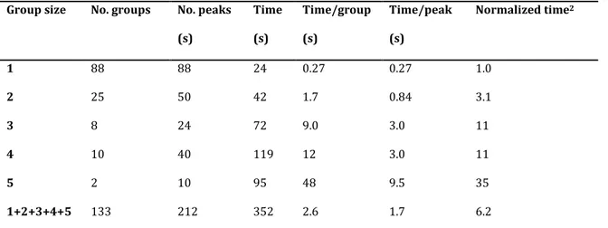
The time required to integrate all peaks in a spectrum depends on the total number of peaks, the data sizes in all dimensions, the number of overlapped groups and the number of peaks in such groups. To benchmark PINT we integrated the peaks of the kinase domain EphB2 that comprises 289 residues (Figure 1). Of the 212 peaks that were possible to integrate, there were 88 well-resolved peaks as well as 25 groups of two, eight groups of three, ten groups of four and two groups of five overlapped peaks. The results are summarized in Table 2.

Table 2. Performance of PINT1

Group size No. groups No. peaks (s) Time (s) Time/group (s) Time/peak (s) Normalized time2 1 88 88 24 0.27 0.27 1.0 2 25 50 42 1.7 0.84 3.1 3 8 24 72 9.0 3.0 11 4 10 40 119 12 3.0 11 5 2 10 95 48 9.5 35 1+2+3+4+5 133 212 352 2.6 1.7 6.2

1_{CPMG experiment of the kinase domain from EphB2. Integration of a data set comprising 21 planes on a Dell}

Precision T1500, Intel(R) Core(TM) i7 Core 870@2,93 GHz. 2_{Time per peak relative to time per peak for}

non-overlapped peaks.

The peaks of this challenging example were integrated in less than six minutes. Not surprisingly, it is usually costly to increase the size of overlapped groups but as can be seen by comparing the results for groups of three and four peaks, speed also depends on how far the starting parameters are from the optimized values. This is also illustrated in the result

25 for the two groups comprising five peaks. One of them required 85 s for integration while the other was integrated in only 10 s. This means that in favorable cases overlapped groups of significantly larger size can be handled in a reasonable amount of time enabling applications to for instance unfolded proteins.

The motivation to use PINT instead of similar programs such as nlinLS (Delaglio et al. 1995) and FuDA (http://pound.med.utoronto.ca/~flemming/fuda/) is based on increased versatility, flexibility and user friendliness rather than improved performance. In contrast it is of interest to compare the performance of PINT with that of ones that use other strategies for peak integration. We therefore compared it with the software Sparky (Goddard and Kneller). Sparky has convenient routines for measurements of peak heights, integration of peak volumes and fitting of exponential decays, and as opposed to PINT it optimizes peak positions and line widths separately for the different spectra that are integrated. We first used Sparky to recalculate the parameters shown in Figure 8A, i.e. R1 rate constants for the

SH3 domain from Abp1p, using both peak heights and peak volumes obtained by integration using default settings. The results are virtually identical for almost all peaks (see supplementary information, Figure 1) demonstrating that the two programs work equally well for uncomplicated spectra.

The advantage of integrating peaks globally (PINT) rather than separately for each spectrum (Sparky) is however obvious for more complicated spectra as shown when we used Sparky to integrate the peaks for the CPMG experiment of the kinase domain from EphB2 (Figure 9). While the speed of integration was comparable, 365 s compared with 352 s for PINT, the quality of the integration was superior for PINT. First, while PINT was able to integrate all 228 peaks in the peak list, successful integration in all 21 planes was only achieved for 155 peaks using Sparky. Second, the integration using Sparky resulted in significantly more scattered data, especially for overlapped peaks (see supplementary information, Figure 2). We also point out that while conversion of peak volumes to effective transverse relaxation rates and fitting of these to the Bloch-McConnell equations for two-site exchange only require three lines in a PINT parameter file, auxiliary programs are needed to do the same for peak volumes obtained from Sparky and indeed from most other programs.

26

Concluding remarks

In conclusion, we have developed the software PINT for integration of peaks in NMR spectra and downstream analysis. The program is a stand-alone application but we recommend using it together with the software Gnuplot since it is convenient to inspect the fits visually. PINT is easy to use and can be customized in a systematic manner until satisfactory results are achieved. Often very little customization is needed to integrate problematic peaks such as ones that are heavily overlapped. The most common relaxation experiments such as measurements of R1, R2, R1ρ, the heteronuclear NOE and CPMG relaxation dispersion are

conveniently analyzed within the program. The speed of the program necessarily depends on the amount of data that have to be analyzed, both in number of data points and number of arrayed planes. In general, the procedure takes from a few seconds to several minutes to complete on a modern PC. We believe that PINT will be a useful tool for speeding up and streamlining integration of peak volumes and analyzing relaxation experiments.

Files included in the distribution

The package can be downloaded from http://www.liu.se/forskning/foass/patrik-lundstrom?l=en. The package contains binaries for a selection of Linux/Unix distributions, a manual and examples of parameter files designed for different purposes. The program Gnuplot that is used for visually inspecting the fitted line shapes is not included but it can be downloaded free of charge from http://www.gnuplot.info/download.html.

Supplementary information

Two figures showing how PINT compares with Sparky.

Acknowledgments

27 and Annica Theresia Blissing for critical reading of the manuscript. The Swedish NMR Center is acknowledged for kindly allowing us to use their spectrometers. This work was supported by a grant from the Swedish Research Council to P.L.

References

Carr HY, Purcell EM (1954) Effects of diffusion on free precession in nuclear magnetic resonance experiments. Phys Rev 94:630-638

Clore GM, Szabo A, Bax A, Kay LE, Driscoll PC, Gronenborn AM (1990) Deviations from the simple two-parameter model-free approach to the interpretation of 15_{N nuclear}

magnetic relaxation of proteins. J Am Chem Soc 112:4989-4991

Delaglio F, Grzesiek S, Vuister GW, Zhu G, Pfeifer J, Bax A (1995) NMRPipe - a multidimensional spectral processing system based on unix pipes. J Biomol NMR 6:277-293

Dempsey CE (2001) Hydrogen exchange in peptides and proteins using NMR-spectroscopy. Prog Nucl Mag Res Sp 39:135-170

Drubin DG, Mulholland J, Zhu ZM, Botstein D (1990) Homology of a yeast actin-binding protein to signal transduction proteins and myosin-I. Nature 343:288-290

Gale NW, Holland SJ, Valenzuela DM, Flenniken A, Pan L, Ryan TE, Henkemeyer M, Strebhardt K, Hirai H, Wilkinson DG, Pawson T, Davis S, Yancopoulos GD (1996) Eph receptors and ligands comprise two major specificity subclasses and are reciprocally compartmentalized during embryogenesis. Neuron 17:9-19

Goddard TD, Kneller DG SPARKY 3. San Francisco.

Hansen DF, Vallurupalli P, Kay LE (2008) An improved 15_{N relaxation dispersion experiment}

for the measurement of millisecond time-scale dynamics in proteins. J Phys Chem B 112:5898-5904

Koradi R, Billeter M, Engeli M, Guntert P, Wuthrich K (1998) Automated peak picking and peak integration in macromolecular NMR spectra using AUTOPSY. J Magn Reson 135:288-297

Korzhnev DM, Ibraghimov IV, Billeter M, Orekhov VY (2001) MUNIN: application of three-way decomposition to the analysis of heteronuclear NMR relaxation data. J Biomol NMR 21:263-8

Lila T, Drubin DG (1997) Evidence for physical and functional interactions among two Saccharomyces cerevisiae SH3 domain proteins, an adenylyl cyclase-associated protein and the actin cytoskeleton. Mol Biol Cell 8:367-385

Lipari G, Szabo A (1982a) Model-free approach to the interpretation of nuclear magnetic-resonance relaxation in macromolecules.1. Theory and range of validity. J Am Chem Soc 104:4546-4559

Lipari G, Szabo A (1982b) Model-free approach to the interpretation of nuclear magnetic-resonance relaxation in macromolecules. 2. Analysis of experimental results. J Am Chem Soc 104:4559-4570

Carr-Purcell-Meiboom-28 Gill sequence for characterizing chemical exchange by NMR spectroscopy. J Am Chem Soc 121:2331-2332

McConnell HM (1958) Reaction rates by nuclear magnetic resonance. J Chem Phys 28:430-431

Meiboom S, Gill D (1958) Modified spin-echo method for measuring nuclear relaxation times. Rev Sci Instrum 29:688-691

Mittermaier A, Kay LE (2006) New tools provide new insights in NMR studies of protein dynamics. Science 312:224-228

Mosteller F, Tukey JW (1977). Data analysis and regression, Addison-Wesley Publishing Company, Reading, MA, p

Mulder FAA, Skrynnikov NR, Hon B, Dahlquist FW, Kay LE (2001) Measurement of slow (µs-ms) time scale dynamics in protein side chains by 15_{N relaxation dispersion NMR}

spectroscopy: Application to Asn and Gln residues in a cavity mutant of T4 lysozyme. J Am Chem Soc 123:967-975

Press WH, Flannery BP, Teukolsky SA, Vetterling WT (1988). Numerical Recipes in C, University Press, Cambridge, p

Rath A, Davidson AR (2000) The design of a hyperstable mutant of the Abp1p SH3 domain by sequence alignment analysis. Protein Sci 9:2457-2469

Romano R, Paris D, Acernese F, Barone F, Motta A (2008) Fractional volume integration in two-dimensional NMR spectra: CAKE, a Monte Carlo approach. J Magn Reson 192:294-301

Stambulchik E (1998) Grace.