Simulation of Surrounding Vehicles in Driving Simulators

Simulation of Surrounding Vehicles in

Driving Simulators

Johan Olstam

Link¨oping studies in science and technology. Dissertations, No. 1248 Copyright c° 2009 Johan Olstam, unless otherwise noted

ISBN 978-91-7393-660-6 ISSN 0345-7524 Printed by LiU-tryck, Link¨oping 2009

Driving simulators and microscopic traffic simulation are important tools for making evaluations of driving and traffic. A driving simulator is de-signed to imitate real driving and is used to conduct experiments on driver behavior. Traffic simulation is commonly used to evaluate the quality of service of different infrastructure designs. This thesis considers a different application of traffic simulation, namely the simulation of surrounding vehicles in driving simulators.

The surrounding traffic is one of several factors that influence a driv-er’s mental load and ability to drive a vehicle. The representation of the surrounding vehicles in a driving simulator plays an important role in the striving to create an illusion of real driving. If the illusion of real driving is not good enough, there is an risk that drivers will behave differently than in real world driving, implying that the results and conclusions reached from simulations may not be transferable to real driving.

This thesis has two main objectives. The first objective is to develop a model for generating and simulating autonomous surrounding vehicles in a driving simulator. The approach used by the model developed is to only simulate the closest area of the driving simulator vehicle. This area is divided into one inner region and two outer regions. Vehicles in the inner region are simulated according to a microscopic model which includes sub-models for driving behavior, while vehicles in the outer re-gions are updated according to a less time-consuming mesoscopic model. The second objective is to develop an algorithm for combining au-tonomous vehicles and controlled events. Driving simulators are often used to study situations that rarely occur in the real traffic system. In order to create the same situations for each subject, the behavior of the surrounding vehicles has traditionally been strictly controlled. This of-ten leads to less realistic surrounding traffic. The algorithm developed makes it possible to use autonomous traffic between the predefined con-trolled situations, and thereby get both realistic traffic and concon-trolled events. The model and the algorithm developed have been implemented and tested in the VTI driving simulator with promising results.

Den h¨ar avhandlingen handlar om att kombinera mikroskopisk trafik-simulering och k¨orsimulatorer. Mikroskopisk trafiktrafik-simulering ¨ar ett vik-tigt verktyg som framf¨orallt anv¨ands f¨or att analysera olika f¨orslag till f¨or¨andringar i v¨agtrafiksystemet. Det kan handla om att j¨amf¨ora olika korsnings- och v¨agutformningar eller trafiksignalsstrategier. I en mikro-skopisk trafiksimuleringsmodell simuleras enskilda f¨orar-fordonsenheter. Simuleringen bygger p˚a delmodeller som beskriver hur f¨orare accelererar, n¨ar de v¨aljer att byta k¨orf¨alt, vilken hastighet de vill k¨ora i, med mera. En k¨orsimulator ¨ar en modellkonstruktion som ska efterlikna verklig bilk¨orning. F¨oraren k¨or fordonet p˚a samma s¨att som ett riktigt for-don, medan den omgivande trafikmilj¨on simuleras. En k¨orsimulator kan liknas vid ett avancerat datorbilspel. K¨orsimulatorer anv¨ands bland an-nat f¨or att studera f¨orarbeteende. Den omgivande trafikmilj¨on spelar en viktig roll i arbetet med att skapa en illusion av verklig bilk¨orning. Om inte illusionen ¨ar tillr¨ackligt bra finns en risk att testpersonerna k¨or annorlunda i k¨orsimulatorn j¨amf¨ort med hur de k¨or i verklig trafik.

I den h¨ar avhandlingen presenteras en modell f¨or att generera och simulera omgivande trafik i en k¨orsimulator. Modellen ¨ar baserad p˚a mikroskopisk trafiksimulering. K¨orsimulatorer anv¨ands ofta f¨or att stud-era situationer eller h¨andelser som s¨allan f¨orekommer i det verkliga trafiksystemet, till exempel trafiks¨akerhetskritiska h¨andelser. F¨or att s¨akerst¨alla att alla f¨ors¨okspersoner k¨or under samma f¨oruts¨attningar brukar de omgivande fordonens beteende strikt kontrolleras. Detta g¨or det m¨ojligt att uts¨atta samtliga f¨ors¨okspersoner f¨or samma situationer. Det medf¨or dock ofta att de omgivande fordonen beter sig mindre likt verkliga bilf¨orare. Genom att anv¨anda en mikroskopisk trafiksimuler-ingsmodell kan realismen ¨okas. Detta medf¨or dock att f¨oruts¨attningarna p˚a detaljniv˚a kommer att skilja sig ˚at mellan f¨ors¨okspersonerna samt att det ¨ar sv˚arare att uts¨atta f¨orarna f¨or f¨orutbest¨amda situationer. F¨or att l¨osa detta har en modell som kan v¨axla mellan simulerad trafik och f¨orutbest¨amda situationer utvecklats. De utvecklade modellerna har im-plementerats och testats i VTIs k¨orsimulator med lovande resultat.

This thesis is the result of research carried out at the division of Commu-nication and Transport Systems at Link¨oping University (LiU) and the Swedish National Road and Transport Research Institute (VTI). The re-search has been sponsored by the Swedish Road Administration through the Swedish Network of Excellence Transport Telematics Sweden.

First of all I would like to thank my supervisor Jan Lundgren for his encouragement, support and guidance. I’m also grateful to my addi-tional supervisors Jonas Jansson, Mikael Adlers and Pontus Matstoms. Thanks also to Laban K¨allgren (VTI) for his priceless help with the integration with the VTI Driving Simulator III.

I would also like to show my appreciation to my colleagues at LiU and VTI, who make LiU and VTI stimulating places to work at. Special thanks to my friend and former roommate Andreas Tapani and to my other Ph. D. student colleagues for very interesting and useful discus-sions, to Arne Carlsson for sharing his knowledge of the traffic theory and simulation area, to Selina M˚ardh and Anne Bolling for their help during the design and the realization of the driving simulator exper-iments conducted, and to the members of the VTI driving simulator group for sharing their massive experience within the driving simulator area.

I would also like to thank St´ephane Espi´e for our fruitful collab-oration and for inviting me to come to Paris and work at his group at INRETS. Thanks also to Jenny Simonsson whom I started this work with during our master thesis and to Ingmar Andr´easson who has kindly read and commented on the thesis draft.

Finally, I would like to express my gratitude to my family and friends for their encouragement and support. Last but not least, thank you Lin for all your love and support.

Norrk¨oping, March 2009 Johan Olstam

1 Introduction 1

2 Traffic simulation 5

2.1 Classification of traffic simulation models . . . 5

2.2 Microscopic traffic simulation . . . 6

2.3 Behavioral model survey . . . 8

2.3.1 Car-following models . . . 9

2.3.2 Lane-changing models . . . 17

2.3.3 Overtaking models . . . 25

2.3.4 Speed adaptation models . . . 28

3 Surrounding vehicles in driving simulators 31 3.1 Driving simulator experiments . . . 32

3.1.1 Scenarios, events and experimental designs . . . . 32

3.1.2 Design issues . . . 34

3.2 Differences compared to traditional applications of traffic simulation . . . 35

3.3 Common modeling approaches . . . 37

3.3.1 Rule based models . . . 40

3.3.2 State machines . . . 41

3.3.3 The eco-resolution principle . . . 43

4 The present thesis 45 4.1 Objectives . . . 45 4.2 Contributions . . . 46 4.3 Delimitiations . . . 47 4.4 Summary of papers . . . 48 4.5 Future research . . . 54 Bibliography 57

Microscopic traffic simulation, henceforth called micro or traffic simu-lation models, has become a powerful and cost-efficient tool for investi-gating traffic systems. Traffic simulation models incorporate sub-models for acceleration, speed adaptation, lane-changing, etc., to describe how vehicle–driver units move and interact with each other and with the in-frastructure. The sub-models, henceforth called behavioral models, use the current road and traffic situation as input and generate individual driver decisions for example with regard to which acceleration rate to apply and which lane to travel in as output. Traffic simulation models offer the possibility to experiment with an existing or a future traffic system in a safe and non disturbing way. The traditional applications of traffic simulation are quality of service evaluations of different road as well as traffic control designs. Common output measures are average speed, flow, density, travel time, delay and queue length. Lately, there has been an increased focus on new applications of traffic simulation. Examples include analysis of Intelligent Transportation Systems (ITS) and traffic management strategies, as well as traffic simulation based safety and environmental impact analyses. There is also an increased focus on combining traffic simulation models and driving simulators, which is the focus of this thesis.

A driving simulator is designed to imitate driving a real vehicle. The driver interface can be realized with a real vehicle cabin or only a seat with a steering wheel and pedals, and anything in between. The surroundings are presented for the driver on a screen and, if available, in rear mirrors. A vehicle model is used to calculate the simulator vehicle’s movements according to the driver’s use of the steering wheel and the pedals. Some driving simulators use a motion system to support the driver’s visual impression of the simulator vehicle’s movements. Last but not least, a driving simulator includes a scenario module that includes the specification of the road, the environment, and all the other actors and events.

areas. Examples include alcohol, medicines and drugs, driving with dis-abilities, human-machine interaction, fatigue, road and vehicle design. Driving simulators can also be used for training purposes. One example is the TRAINER simulator (Gregersen et al., 2001) that was developed to work as a complimentary vehicle in driving schools. Driving simu-lators offer possibilities to practice actions that are unsafe, difficult or impossible to train in the real road network. This could be anything between basic maneuvering to emergency situations.

It is important that the performance of the simulator vehicle, the visual representation, and the behavior of surrounding objects are re-alistic, in order for a driving simulator to be a valid representation of real driving. For example, it is important that the surrounding vehicles behave in a realistic and trustworthy way. Surrounding vehicles influ-ence a driver’s mental load and ability to drive a vehicle. It is not only important that the behavior of a single driver is realistic, but also that the behavior of the whole traffic stream is realistic. For instance, drivers who drive fast expect to catch up with more vehicles than the number of vehicles that catch up with them and vice versa.

A realistic simulation of surrounding vehicles, and thereby traffic, can be achieved by combining a driving simulator with a model for mi-croscopic simulation of traffic. However, traffic simulation models have traditionally not been used to simulate surrounding vehicles in driving simulators. The usual approach has instead been to strictly control the behavior of the surrounding vehicles. It is desirable for several reasons to keep the variation in test conditions between different drivers (henceforth called subjects) as low as possible. Traffic simulation models simulate autonomous vehicles, and by using autonomous surrounding vehicles, subjects will experience different situations at the microscopic level de-pending on how they drive. The use of autonomous vehicles makes it difficult to limit the variation in test conditions. The subjects’ condi-tions will still be comparable at a higher, more aggregated, level, e. g. comparable traffic densities and average speeds. Whether comparable conditions at an aggregated level are sufficient or not varies depending on the type of experiment. For some experiments, comparable condi-tions at the microscopic level are essential, and it may not be suitable to use autonomous vehicles. In other experiments, comparable conditions at a higher level are sufficient. A related problem is that the use of autonomous surrounding vehicles also makes it more difficult to expose the subject to specific controlled situations or events.

and controlled events. The thesis is organized as follows. Chapter 2 gives an introduction to the field of traffic simulation. The chapter in-cludes a survey of commonly used behavioral models for car-following, lane-changing, overtaking, and speed adaptation. Chapter 3 gives an introduction to the field of simulating surrounding vehicles in driving simulators. The chapter starts with an introduction to driving simu-lator experiments, then follows a discussion on the differences between this application and more traditional applications of traffic simulation. The chapter ends with a survey of the most commonly used modeling approaches for simulating surrounding vehicles in driving simulators.

Chapter 4 presents the objectives, contributions, and delimitations of this thesis. The chapter also includes summaries of the five papers included and suggestions for future research.

The societies of today need well functioning traffic and transportation systems. Congestion and traffic jams have become recurrent problems in most of the larger cities and also more common in smaller cities. In order to avoid congestion and to optimize the traffic systems with re-spect to capacity, accessibility and safety, traffic planners need tools that can predict the effects of different road designs, management strategies, and increased travel demands. Therefore, in recent decades researchers and developers have developed many different types of models and tools that deal with these kinds of issues. The rapid development in the per-sonal computer area has created new possibilities to develop enhanced traffic modeling tools. Traffic models are mainly based on analytical or simulation approaches. The analytically models often use queue theory, optimization theory or differential equations that can be solved analyt-ical to model road traffic. These kinds of models are mainly used to study average situations and offer limited possibilities for studying how the dynamics of a traffic system varies over time. Simulation models on the other hand, offer good possibilities for this.

2.1

Classification of traffic simulation models

There are many different kinds of traffic models and there are also dif-ferent ways to classify traffic models. Traffic simulation models are typ-ically classified according to the level of detail at which they represent the traffic stream. Three categories are generally used, namely: Micro-scopic, Mesoscopic and Macroscopic.

Microscopic models represent the traffic stream at a high level of de-tail. They model individual vehicles and the interaction between them. Microscopic models incorporate sub-models for acceleration, speed adap-tation, lane-changing, gap acceptance etc., to describe how vehicles move and interact with each other and with the infrastructure. Several models have been developed and the most well-known are probably AIMSUN

(Barcel´o and Casas, 2002; TSS, 2008), VISSIM (PTV, 2008), Param-ics (Quadstone, 2004; Quadstone ParamParam-ics, 2008), MITSIMLab (Toledo et al., 2003), and CORSIM (FHWA, 1996).

Mesoscopic models often represent the traffic stream at a rather high level of detail, either by individual vehicles or packets of vehicles. The difference compared to micro models is that interactions are modeled with lower detail. The interactions between vehicles and the infras-tructure are typically based on macroscopic relationships between flow, speed and density. Examples of mesoscopic simulation models are DY-NASMART (Jayakrishnan et al., 1994), CONTRAM (Taylor, 2003), DYNAMEQ (Florian et al., 2006), and MEZZO (Burghout, 2004).

Macroscopic models use a low level of detail, both with regard to the representation of the traffic stream and interactions. Instead of modeling individual vehicles, the macro models use aggregated variables such as flow, speed and density to characterize the traffic stream. Macro models commonly use speed–flow relationships and conservation equations to model how traffic propagates through the network modeled. Examples of macroscopic simulation models are METANET/METACOR (Papa-georgiou et al., 1989; Salem et al., 1994) and the Cell Transmission model (Daganzo, 1994, 1995).

2.2

Microscopic traffic simulation

Microscopic traffic simulation models simulate individual vehicles. The general approach is to treat a driver and a vehicle as one unit. As in reality, these vehicle–driver units interact with each other and with the surrounding infrastructure. Micro models consist of several sub-models, henceforth called behavioral sub-models, that each handle specific interactions. The most essential behavioral model is the car-following model, which handles the longitudinal interaction with preceding ve-hicles. Other important behavioral models include models for lane-changing, gap-acceptance, overtaking, ramp merging, and speed adapta-tion. The sub-models required depend on the type of road that the model is designed for. Lane-changing models are for instance only necessary when simulating urban or freeway environments and are not required in models for two lane highways with oncoming traffic. The most common behavioral models will be presented in more detail in Section 2.3.

Most micro models are designed for simulating urban or freeway net-works. The most well known models for these environments are the ones

presented in Section 2.1 (AIMSUN, VISSIM, Paramics, MITSIMLab, and CORSIM). Only a few models for two-lane highways with oncoming traffic have been developed. The state-of-the-art in rural road models includes the Two-Lane Passing (TWOPAS) model (Leiman et al., 1998), the Traffic on Rural Roads (TRARR) model (Hoban et al., 1991), and the VTISim model (Brodin and Carlsson, 1986). The VTISim model has been further developed in the Rural Road Traffic Simulator (RuTSim) model (Tapani, 2005, 2008).

In order to model how behavior and preferences vary among drivers, each vehicle–driver unit is assigned different vehicle and driver charac-teristics. These characteristics commonly include vehicle length, desired speed, desired following distance, possible or desired acceleration and deceleration rates, etc. The variation among the population is generally described by a distribution function and individual parameter values are drawn from the specified distribution. For example, we can assume that the desired speeds on freeways follow a normal distribution with a mean of 111 km/h and a standard deviation of 11 km/h. Micro models are generally time discrete, but some event based models have also been developed, see for instance Brodin and Carlsson (1986). In event based models, vehicles are only updated in the case of an event, e. g. when catching up with a preceding vehicle. The basic principle of a time dis-crete model is that the time is divided into small time steps, commonly between 0.1 and 1 seconds. At each time step, the model updates every vehicle according to the set of behavioral models. At the end of the time step, the simulation clock is increased and the simulation enters the next time step.

Microscopic simulation models have traditionally been used to con-duct capacity and quality of service evaluations of different road designs and management strategies. During the last decade, micro models have also been used to a greater extent to evaluate different ITS-applications, for example Intelligent Speed Adaptation (Liu and Tate, 2000) or Adap-tive Cruise Control systems (Champion et al., 2001; Kesting et al., 2007b; Tapani, 2008). Research has also been conducted within the area of combining micro simulation and different safety indicators to perform safety analysis of different road and intersection designs, see for example Archer (2005) and Gettman and Head (2003).

Even though micro models work on a micro level and simulate in-dividual vehicles, they have mainly been used to generate macroscopic outputs such as average speeds, flows, and travel times. A large part

of the calibration and validation of micro models is therefore generally performed at a macroscopic level. The different behavioral models have been calibrated and validated to various extents at a micro level. How-ever, little effort has been put into calibrating and validating combina-tions of behavioral models at a micro level, for example if a car-following model in combination with a lane-changing model generates valid results at a micro level.

2.3

Behavioral model survey

In order to be usable and perform well, traffic simulation models have to be based on high-quality behavioral models. To generate realistic behavior is of course the most important property of a good behavioral model, but it is not the only desirable property. A realistic behavioral model is of little or no use if it cannot be calibrated or if this task is too time-consuming. It is therefore desirable to keep the number of model parameters as low as possible. When designing a behavioral model, the aim should be to find the best compromise between the number of pa-rameters and output agreement. It is also desirable that the papa-rameters used can easily be interpreted as known vehicle or driver factors. This simplifies the calibration work and allows the user to experiment, in a more straightforward and easy way, with different parameter settings with regard to the variation in behavior among drivers for example.

Different road environments require different kinds of behavioral models. A traffic simulation model for urban roads must include dif-ferent types of behavioral models than a simulation model for rural environments. However, common to all environments is the need of a car-following model. A car-following model describes a vehicle–driver unit’s acceleration with respect to preceding vehicles in the same lane, the driver’s own goals and the vehicle’s acceleration capabilities. An-other behavioral model that is necessary in all road environments, is a speed adaptation model, which calculates a driver’s preferred or desired speed along the road. In urban and freeway environments, models for lane-changing decisions are essential. However, on two-lane highways, a model that considers the whole overtaking procedure is required. Such a model cannot only deal with the lane change to the oncoming lane. It also has to consider the actual passing procedure when the vehicle is traveling in the oncoming lane and the lane change back into its own lane. As a part of both lane-changing and overtaking models, some type

of gap-acceptance model is necessary. A Gap-acceptance model con-trols the decision to accept or reject an available gap, for example if a vehicle–driver unit that desires to change lane accepts the available gap between two subsequent vehicles in the target lane. Some kind of gap-acceptance model is also necessary when modeling intersections, lane drops or on-ramp merging situations.

The following sections will describe different kinds of car-following, lane-changing, overtaking, and speed adaptation models in more detail. The sections also include descriptions of different approaches to gap-acceptance in connection to lane-changes and overtakings.

2.3.1 Car-following models

A car-following model controls a driver’s behavior with respect to pre-ceding vehicles in the same lane. A vehicle–driver unit is classified as

following when it is constrained by a preceding vehicle, and when

driv-ing at the desired speed will lead to a collision. When a vehicle–driver unit is not constrained by another vehicle, it is considered free and trav-els, in general, at its desired speed. The follower’s action is commonly specified through the follower’s acceleration, although some models, for example the car-following model by Gipps (1981), specify the follower’s actions through the follower’s speed. Some car-following models only de-scribe drivers’ behavior when they are actually following another vehicle, whereas other models are more complete and determine the behavior in all situations. In the end, a car-following model should deduce both in which regime or state a vehicle–driver unit is, and what actions it applies in each state.

Most car-following models use several regimes to describe the fol-lower’s behavior. A common setup is to use three regimes: one for free driving, one for normal following, and one for emergency deceleration. In the free regime, vehicle–driver units are unconstrained and try to achieve their desired speed, whereas in the following regime they adjust their speed with respect to the vehicle in front. Vehicles in the emergency deceleration regime decelerate to avoid a collision. Most car-following models consider only the interaction with the closest preceding vehi-cle. However, there are reports (see e. g. Hoogendoorn et al., 2006) that indicate that car-following models including several leaders fit empiri-cal data better than models that include only one leader. An example of a model that includes several leaders is the Human Driver Model

(Treiber et al., 2006). The interested reader can consult Brackstone and McDonald (1998) for a historical review of car-following models and Jan-son Olstam and Tapani (2004) for a more detailed description of some of the car-following models presented in this section. The following no-tation will be used throughout this section to describe the car-following models, see also Figure 2.1:

a_n acceleration, vehicle n, [m/s2_] xn position, vehicle n, [m] vn speed, vehicle n, [m/s] ∆x x_n−1− x_n, space headway, [m] ∆v vn− vn−1, approach speed, [m/s] vdes

n desired speed, vehicle n, [m/s] L_n−1 length of vehicle n − 1, [m]

sn−1 effective length (Ln−1 + minimum gap between

stationary vehicles), vehicle n − 1, [m]

T reaction time, [s] n n − 1 -Driving direction -¾Ln−1 -¾ xn -¾ xn−1

Figure 2.1: Car-following notation.

Classification of car-following models

Car-following models are commonly divided into classes or types depend-ing on the logic utilized. The Gazis–Herman–Rothery (GHR) family of models is probably the model class that has been studied most. The GHR model is sometimes referred to as the general car-following model. The first version was presented in 1958 (Chandler et al., 1958) and sev-eral enhanced versions have been presented since then. The GHR model

only controls the actual following behavior. The basic relationship be-tween a leader and a follower vehicle in this case is a stimulus-response type of function. The GHR model states that the follower’s accelera-tion depends on the speed of the follower, the speed difference between the follower and the leader, and the space headway (Brackstone and McDonald, 1998). That is, the acceleration of the follower at time t is calculated as

an(t) = α · vnβ(t) ·

v_n−1(t − T ) − v_n(t − T )

(xn−1(t − T ) − xn(t − T ))γ, (2.1)

where α > 0, β and γ are model parameters that control the propor-tionalities. A GHR model can be symmetrical or unsymmetrical. A symmetrical model uses the same parameter values in both accelera-tion and deceleraaccelera-tion situaaccelera-tions, whereas an unsymmetrical model uses different parameter values in acceleration and deceleration situations. An unsymmetrical GHR-model is used for instance in MITSIM (Yang and Koutsopoulos, 1996) to calculate the acceleration in the following regime, and it is formulated as

an(t) = α±· vβ ± n (t) ·

v_n−1(t − T ) − v_n(t − T )

(x_n−1(t − T ) − l_n−1− x_n(t − T ))γ±, (2.2) where α±_{, β}± _{and γ}± _{are model parameters. The parameters α}+_{, β}+

and γ+ _{are used if v}

n≤ vn−1 and α−, β− and γ− are used if vn> vn−1.

Besides the following regime, the MITSIM model uses an emergency regime and a free driving regime.

The safety distance or collision avoidance models constitute another type of car-following models. In these models, the driver of the following vehicle is assumed to always try to keep a safe distance to the vehicle in front. Pipes’ rule which says:

”A good rule for following another vehicle at a safe dis-tance is to allow yourself at least the length of a car between you and the vehicle ahead for every ten miles of hour speed at which you are traveling” (Hoogendoorn and Bovy, 2001), is a simple example of a safety distance model. The safe distance is com-monly specified through manipulations of Newton’s equations of motion. In some models, this distance is calculated as the distance that is nec-essary to avoid a collision if the leader decelerates heavily. The most

well known safety distance model is probably the one by Gipps (1981). In this model, the follower chooses the minimum speed of the one con-strained by the follower’s own vehicle and the one concon-strained by the leader vehicle, that is the minimum of

va_n(t + T ) = vn(t) + 2.5 · amT · µ 1 −vn(t) vdes n ¶ · s 0.025 +vn(t) vdes n (2.3) and v_nb(t + T ) = dmT + Ã (dmT )2 " vn−1(t)2 ˆ dn−1 # −dm " 2 (∆x (t) − sn−1) − vn(t) T −vn−1(t) 2 ˆ dn−1 #!_0.5 . (2.4)

Here am _{and d}m _{is the maximum desired acceleration and deceleration}

for vehicle n, respectively, and ˆd_n−1 is an estimation of the maximum deceleration desired by vehicle n − 1. The safe speed with respect to the leader (Equation 2.4) is derived from the Newtonian equations of motion. The equation calculates the maximum speed that the follower can drive at and still, after some reaction time, be able to decelerate down to zero speed and avoid a collision if the leader decelerates down to zero speed. Another safety distance model is the Intelligent Driver Model (IDM) by Treiber et al. (2000). The IDM also consists of one function for the acceleration with respect to the follower’s own vehicle and one function for the acceleration with respect to the leader. In the IDM, the two functions are added together into one function as

an= a0 " 1 − µ vn vdes n ¶₄ − µ s∗(vn, ∆v) s ¶₂# , (2.5) where s∗(v, ∆v) = s₀+ v_n· Tdes+ vn∆v 2√a0b . (2.6)

Here s = ∆x − Ln−1 and the parameter a0 and b determines maximum

acceleration and deceleration, respectively. The parameter s0 is the

minimum distance between stationary vehicles and T_d is the desired following time gap.

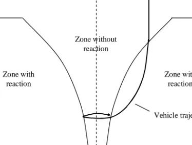
In 1963 a new approach for car-following modeling were presented, (Brackstone and McDonald, 1998). Models using this approach are clas-sified as psycho-physical or action point models. Psycho-physical models use thresholds or action points where the driver changes his/her behav-ior. Drivers are able to react to changes in spacing or relative veloc-ity only when these thresholds are reached, (Leutzbach, 1988). The thresholds, and the regimes they define, are often presented in a relative space/speed diagram of a follower–leader vehicle pair; see Figure 2.2 for an example. The bold line symbolizes a possible vehicle trajectory.

Zone without reaction 0 ∆v x ∆ Zone with reaction Zone with reaction Vehicle trajectory

Figure 2.2: A psycho-physical car-following model (Source: Leutzbach, 1988).

Representative examples of psycho-physical car-following models are those by Wiedemann (1974); Wiedemann and Reiter (1992), see Figure 2.3, and Fritzsche (1994), see Figure 2.4.

Fuzzy-logic is another approach that to some extent has been utilized in car-following modeling. Fuzzy logic or fuzzy set theory can be used to model drivers’ inability to observe absolute values. For example, human beings cannot deduce exact values of speed or relative distance, but they can give estimations like “above normal speed”, “fast”, “close”, etc. In the models described above, drivers are assumed to know their exact own speed and distance to other vehicles etc. In order to get a more human-like modeling, fuzzy logic models assume that drivers are able to

Emergency regime Following

Upper limit of reaction

0 Free driving Closing in v ∆ x ∆

Figure 2.3: The different thresholds and regimes in the Wiedemann car-following model (Wiedemann, 1974; Wiedemann and Reiter, 1992).

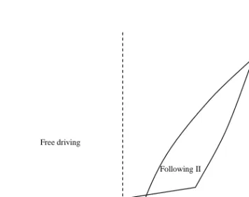
Following II Following I Closing in Free driving 0 ∆v x ∆ Danger

Figure 2.4: The different thresholds and regimes in the Fritzsche car-following model (Fritzsche, 1994).

2.3. BEHAVIORAL MODEL SURVEY

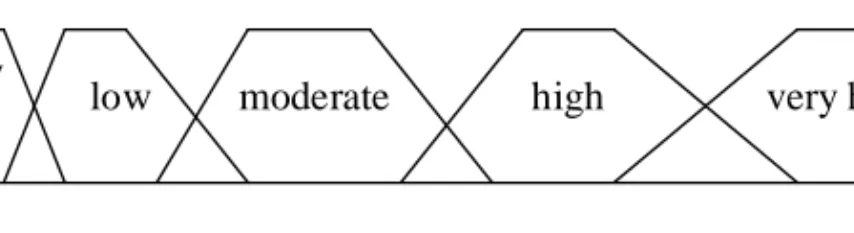
conclude only if the speed of the front vehicle is very low, low, moderate, high, or very high for example. In many cases, the fuzzy sets overlap each other. To deduce how a driver will observe a current variable value, membership functions that map actual values to linguistic values have to be specified, see Figure 2.5 for an example.

speed low moderate very high 0 1 high very low Membership value

Figure 2.5: Example of membership functions for driving speed.

The strength of fuzzy logic is that the fuzzy sets can easily be com-bined with logical rules to construct different kinds of behavioral models. A possible rule can for instance be: if own speed is “low”, desired speed is “moderate” and headway is “large”, then increase speed. As seen in the previous sentence, it is rather easy to create realistic and workable linguistic rules for a specific driving task. However, one big problem is that the fuzzy sets need to be calibrated in some way. There have been attempts to “fuzzify” both the GHR model and a model named MIS-SION (Wiedemann and Reiter, 1992). However, no attempts to calibrate the fuzzy sets have been made, (Brackstone and McDonald, 1998). Model properties

As presented in the previous section, there are different types of car-following models. Several car-car-following models, using different approach-es, have been developed since the 1950’s. Despite the number of models that have already been developed, there is still active research in the area. One reason for this is that the preferred choice of car-following model may differ depending on the application. For example, the re-quirements placed on a car-following model used to generate macroscopic outputs, e. g. average flow and speed, is lower than the requirements on car-following models used to generate microscopic output values, such as individual vehicle trajectories.

Traffic simulation models and thereby car-following models are most-ly utilized to study how changes in a network affect traffic measures such as average flow, speed, density etc. In other words, the simulation output of interest in such applications is macroscopic measures, hence the car-following models utilized should at least generate representative macroscopic results. Leutzbach (1988) presents a macroscopic verifica-tion of GHR-models. Through an integraverifica-tion of the car-following equa-tion it is possible to obtain a relaequa-tionship between average speed, flow and density. This relationship can then be compared to real data or to outputs from other macroscopic models. For a GHR-model with β = 0 and γ = 2, the integration becomes the well recognized Greenshield’s relationship (see e. g. May, 1990):

q = v · k = vdes· µ 1 − k kmax ¶ · k, (2.7)

where q is the traffic flow (vehicles/hour), k is the density (vehicles/km) and kmax is the maximal possible density (jam density). A verification

of this kind however is not possible for an arbitrary car-following model. It is for example not possible to integrate a psycho-physical model, since such models do not express the follower’s acceleration in a mathemat-ically closed form. However, macroscopic relationships can always be generated by running several simulations with different flows.

Drivers’ reaction time is a parameter which is common in most car-following models. It is assumed that with long reaction times, vehicles have to drive with large gaps between each other in order to avoid col-lisions, hence the traffic density, and thereby the flow, will be reduced. Most car-following models use one common reaction time for all drivers. This is not realistic from a micro perspective but may be enough to generate realistic macro results.

The magnitude of drivers’ reactions also influences the simulation results. How the output is affected is not as obvious as in the case of reaction time. High acceleration rates should lead to vehicles reaching their new constraint speed faster, which should decrease the vehicles travel time delay. High deceleration rates should also lead to less travel time delay, and thus the vehicles can start their decelerations later. High acceleration and deceleration rates may however result in oscillat-ing vehicle trajectories in congested situations and thereby decrease the average speed.

be-havior. Firstly, driver characteristics such as reaction time and reaction magnitude vary among drivers. Driving behavior may also vary accord-ing to country or territory, due to different formal and informal drivaccord-ing and traffic rules. For example, drivers in the USA may, for example, not drive in the same way as European or Asian drivers. Behavioral mod-els that are used to model traffic in different countries must therefore offer the possibility of using different parameter settings. The differ-ences between countries may however be so big that even with different parameter values, the same car-following model cannot be used to de-scribe the behavior in two countries with different traffic conditions. See e. g. Tapani et al. (2008) for further reading on simulation modeling of different regions. Furthermore, it may be necessary to use different pa-rameters, or even different models, for different traffic situations, for example congested and non congested traffic. There are versions of the GHR model that use different parameter values for congested and non congested situations, (Brackstone and McDonald, 1998). For example, it is important to remember that driving characteristics such as reac-tion time are often treated as parameters, but that in reality they vary depending on the driving context. Drivers may be more alert in con-gested situations and thereby have a shorter reaction time than in non congested situations. A model that does not include sub-models for how parameters such as reaction time are affected by the driving con-text consequently require different parameter values for different traffic situations.

2.3.2 Lane-changing models

Lane-changing models describe drivers’ behavior when deciding whether to change lane or not on a multi-lane road link. This type of behavioral model is essential and is important both in urban and freeway envi-ronments. When deciding whether to change lane, a driver needs to take several things into consideration. Gipps (1986) proposed that a lane-changing decision is the result of answering the questions

• Is it necessary to change lane?

• Is it desirable to change lane?

• Is it possible to change lane?

Gipps (1986) presented a framework for the structure of lane-changing decisions in the form of a decision tree. The proposed decision tree

considered for instance the driver’s desire to reach the desired speed, the driver’s intended turn, any reserved lanes or obstructions, and the urgency of the lane change in terms of the distance to the intended turn. Several lane-changing models, for example the models by Barcel´o and Casas (2002), Hidas (2002, 2005), and Yang (1997), are based on the three basic steps proposed by Gipps (1986).

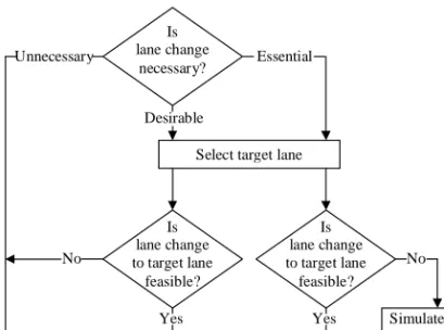
In the model by Gipps (1986) all lane changes are impossible if the gap available in the target lane is smaller than a given limit. This is a reasonable approach when a lane change is desirable. However, in situations where a lane change is necessary or essential but not possible, vehicles in the target lane often help the trapped vehicle by adjusting their speed to create a large enough gap for the trapped vehicle to enter. This behavior has been addressed for instance by Hidas (2002, 2005). Hidas (2002) describes a further developed version of the model by Gipps (1986), which also includes the cooperative behavior for vehicles in the target lane, see Figure 2.6.

Is lane change necessary? Is lane change to target lane feasible? Is lane change to target lane feasible? Select target lane

Simulate driver courtesy in target lane Change to target lane Remain in current lane Unnecessary Essential Desirable Yes No Yes No

Figure 2.6: Structure for lane-changing decisions proposed in Hidas (2002).

In the model structure proposed by Hidas (2002), the necessary and desirable steps are merged into one necessary step with the possible outcomes: unnecessary, desirable, or essential. A similar approach for modeling cooperative lane-changing was proposed by Yang and

Kout-sopoulos (1996). This model classifies a lane change as either mandatory or discretionary. Mandatory lane changes correspond to the essential statement in the model by Hidas (2002), that is lane changes which are necessary in order to pass a lane blockage, reach an intended turn, avoid restricted lanes, etc. The term discretionary lane changes refers to lane changes made in order to gain speed advantages or avoid lanes close to on-ramps, etc. The discretionary lane changes can be compared to the desirable path in the structure by Hidas (2002). In both structures, the differences between mandatory and discretionary lane changes lies in the gap-acceptance behavior and the possibility that vehicles in the target lane may renounce their right of way in favor of a vehicle performing a mandatory lane change.

Toledo et al. (2005) pointed out that in principle, all lane-changing models only consider lane changes to an adjacent lane. The models evaluate whether the driver should change to an adjacent lane or stay in the current one. Thus, most models lack an explicit tactical choice with regard to their lane-changing behavior. Toledo et al. (2005) presented a model in which a driver chooses a target lane, not necessarily an adjacent lane, that is most beneficial for him/her. In this way the driver will strive to reach the most beneficial lane, sometimes which may need several lane changes to achieve. This model follows in principle, the basic decision structure proposed in Gipps (1986). However, the necessary and desired steps are merged into one target lane choice. This is possible since lanes that are less convenient, for example due to the next turning movement, will be less beneficial for the driver. In Toledo et al. (2005) a utility function is used to calculate the benefit of each lane and a discrete choice model is used to model the lane choice. This model will be described in more detail later on in this section when a driver’s desire to change lane is discussed.

El Hadouaj et al. (2000) proposed a similar model as Toledo et al. (2005) in which drivers not only base their lane-changing decisions on the traffic situation in their own and the adjacent lanes, but instead, the decision is based on the situation in all lanes. The model considers not only the traffic situation in the driver’s vicinity but also the situation further away. The area around a driver is divided into several areas, behind, in front and beside the driver. Lane changes are then based on the benefits in the different areas. This benefit is calculated through an assessment function that considers the speed and stability in the different areas around the driver. The model is based on psychological driver

2. TRAFFIC SIMULATION

behavior studies performed at the French research institute INRETS and the Driving Psychology Laboratory (LPC), (El Hadouaj et al., 2000).

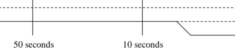
The urgency or necessity to change lane depends on the distance to an obstacle or an intended turn. This can be modeled in several different ways. Gipps (1986) used three different areas, close, middle distance, and remote, defined by two time distances to the intended turn or obstacle, see Figure 2.7 for an example.

Zone 3 - close Zone 2 – middle distance

Zone 1 – remote

50 seconds 10 seconds

Figure 2.7: The three different lane-changing zones proposed by Gipps (1986).

After trials, suitable values of 10 s and 50 s for the two time distances were proposed, (Gipps, 1986). This zone division has later been adopted and further developed by Hidas (2002) and Barcel´o and Casas (2002). A similar zone division has also been presented in Wright (2000). The basic principle is that a vehicle–driver unit in zone 1 is considered far away from its intended turning or from any obstacle, and changes lane if it desires. A vehicle–driver unit in zone 2 is closer to the intended turn and is assumed to be a little bit more restrictive in its lane changing decisions. Vehicle–driver units in zone 2 seldom or never change to lanes further away from the lane suitable for the next turning. In zone 3, all lane-changing decisions exclusively focus on getting to the suitable lane for the next turning. A vehicle in zone 3 that is not traveling in the lane suitable for its intended turning will become more aggressive and start to accept smaller gaps. This will be discussed later under the sub-section about gap-acceptance.

Yang (1997) proposed another way of modeling the urgency of a driver’s need to change lane. Instead of using different zones, vehicles are tagged to mandatory state according to a probability function. In Yang (1997) an exponential probability function was used, in which the probability of tagging a vehicle as mandatory mainly depends on the distance to the intended turning or obstacle. This strategy has also been adopted by Wright (2000), but the exponential distribution was

replaced by a linear relationship in order to save computational time. Modeling drivers’ desire to change lane

A driver’s desire to change lane can be modeled in several ways, for example by using

• A car-following model

• A pressure function

• Discrete choice theory

• Fuzzy logic

In the model proposed by Gipps (1986), a car-following model, more precisely the model presented by Gipps (1981) (see Equation 2.3 and 2.4), was used to calculate which lane has the least effect on the driver’s speed. The model also accounted for the presence of heavy vehicles in the different lanes by calculating the effect of the next heavy vehicle in each lane as if they were the just preceding vehicles in respective lane. The model in Gipps (1986) also includes a relative speed condition for deciding if a driver is willing to change lane. Gipps (1986) used values of 1 m/s and -0.1 m/s for lane changes towards the center and the curb, respectively, i. e. vehicles do not intend to change lane to the left if they are not driving 1 m/s faster than the preceding vehicle in the current lane.

The lane-changing model MOBIL (Minimizing Overall Braking In-duced by Lane change) by Kesting et al. (2007a) also utilizes a car-following model, more precisely the IDM (Treiber et al., 2000) (see Equation 2.5), for calculating the utility or gain of driving in the differ-ent lanes. The IDM is used to compare the acceleration that the driver can use in the different lanes and how a lane change will affect the accel-eration of the current and the presumptive new follower, i. e. the nearest vehicle behind the driver in the evaluated lane.

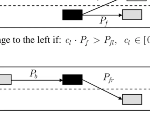
Kosonen (1999) has proposed an approach similar to using a car-following model to evaluate which lane that is preferable. Instead of using the car-following model, a pressure function was defined. This pressure function is an approximation of the potential deceleration rate caused by the leading vehicle and it is defined as

P =

¡

vdes− vobs¢2

where vdes _{is the desired speed, v}obs _{is the obstacle’s speed, and s is}

the relative distance. The pressure function is used to model drivers lane-changing decisions according to the logic described in Figure 2.8. The logic is combined with a minimum time before a new lane change is allowed. This is done in order to avoid to frequent lane-changing behavior. For lane changes to the left, the rule is also combined with a minimum difference in desired speed condition, similar to that used by Gipps (1986). fl P f P b P _Pfr

Change to the left if: c Pl ⋅ f > Pfl, cl ∈[0,1 ]

Change to the right if: c Pr ⋅ b >Pfr, cr ∈[0,1 ]

Figure 2.8: The lane-changing logic proposed by Kosonen (1999). P

is calculated according to Equation 2.8. The parameters c_l and c_r are

calibration parameters, which controls the driver’s willingness to change to the left and right, respectively.

Toledo et al. (2005) presented a model in which the necessary and the desired steps are merged together into a target lane model. The model is based on discrete choice theory and calculates the benefit of each lane by using the utility function

U_intTL = β_iTLX_intTL+ α_iTLvn+ εTLint ∀i ∈ {lane 1, lane 2, . . .} , (2.9)

where UTL

int is the utility of lane i as target lane for driver n at time t. The

vector XTL

int consists of the explanatory variables that affect the utility of

lane i, for example lane density and speed conditions, speed difference to the preceding vehicle etc. The variable vnis an individual-specific latent

variable assumed to follow some distribution in the population. βTL i

and αT L

respectively. In Toledo et al. (2005), the random terms εTL

int are assumed

to be independently identically Gumbel distributed. This leads to that the probability of choosing lane i being given by the multinomial logit model P (TLnt = i| vn) = exp¡VTL int ¯ ¯ vn ¢ P j∈TL exp¡VTL int ¯ ¯ v_n¢

∀i ∈ TL = {lane 1, lane 2, . . .} ,

(2.10)

where VTL int

¯

¯ vnare the conditional systematic utilities of the alternative

target lanes. Toledo et al. (2005) also present an estimation of the model parameters for a road section of I-395 Southbound in Arlington VA., USA.

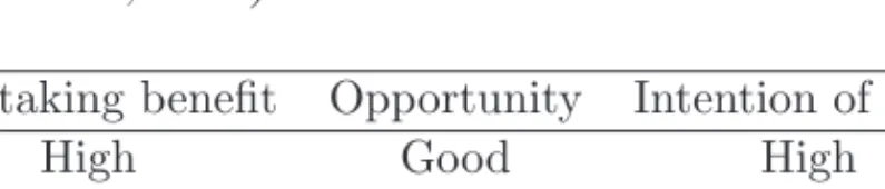
Drivers’ willingness or desire to change lane can also be modeled by using fuzzy logic techniques. Wu et al. (2000) describe a lane-changing model that use the fuzzy sets in Table 2.1 and 2.2 for modeling lane changes to the left (LCO) and right (LCN), respectively.

Table 2.1: Fuzzy sets terms for lane-changing decisions to the off-side/left, (Wu et al., 2000).

Overtaking benefit Opportunity Intention of LCO

High Good High

Medium Moderate Medium

Low Bad Low

Table 2.2: Fuzzy sets terms for lane-changing decisions to the near-side/right, (Wu et al., 2000).

Pressure from Rear Gap satisfaction Intention of LCN

High High High

Medium Medium Medium

Low Low Low

A typical lane-changing rule for changing to the left according to Wu et al. (2000) is:

If Overtaking Benefit is High and Opportunity is Good then Intention of LCO is High

In Wu et al. (2000) triangular membership functions were used for all fuzzy sets. The sets were calibrated to freeway data and quite good agreements of lane-changing rates and lane occupancies were obtained. However, the paper does not include any information about the best-fit parameter values.

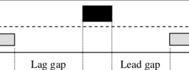
Gap-acceptance

Even if a lane change is desirable and perhaps also necessary it might not be possible or safe to perform it. In order to evaluate whether a driver safely can change lane, some kind of gap-acceptance model is generally used. A driver has to decide whether the gap between two subsequent vehicles in the target lane is large enough to perform a safe lane change. This decision-making is generally modeled as evaluating the available lead and lag gaps, see Figure 2.9.

Lead gap Lag gap

Figure 2.9: Illustration of lead and lag gaps in lane-changing situations.

The common approach is to define a critical gap that determines which gaps drivers accept and which they not accept. In reality, this critical gap varies both among drivers and over time. It also varies between lane changes to the right and to the left and between lead and lag gaps. However, critical gaps are difficult to measure, in principle, only accepted gaps and to some extent rejected gaps can be measured. Thus, it is difficult to measure how critical gaps, for example, vary among drivers and over time for a specific driver. One approach is therefore to use one critical gap for all drivers, but different critical values for lead and lag gaps and for changes to the right and left. This approach is used in the model by Kosonen (1999) for instance. Even though critical gaps are difficult to measure some models have used the approach of using critical gap distributions. For instance, in Ahmed (1999) and later in Toledo et al. (2005) critical gaps are assumed to follow log-normal distributions.

The models by Gipps (1986), Hidas (2002), and Kesting et al. (2007a) are based on a similar but to some extent different approach. Instead of looking at the available and critical gap, a ”critical” (or rather an acceptable) deceleration rate is used. In Gipps (1986) a car-following model, namely the model in Gipps (1981), was used to calculate the deceleration rate required to change lane into the available gap. This deceleration rate was compared to an acceptable deceleration rate. If the deceleration rate required was unacceptable to the driver, the lane change is not feasible. For lead gaps, the car-following model was applied on the subject vehicle with the preceding vehicle in the target lane as leader. For lag gaps, the car-following model was applied on the lag vehicle in the target lane with the subject vehicle as the leader vehicle. The gap-acceptance model also has an important role in the modeling of the urgency of a lane change. When getting closer to an obstacle or an intended turn, i. e. when in zone 2 or 3 in Figure 2.7, it is more urgent for drivers to get to the target lane. In these situations, drivers generally accept smaller gaps, or following the approach in Gipps (1986), Hidas (2002), and Kesting et al. (2007a) higher deceleration rates. In Yang and Koutsopoulos (1996) this is modeled by a linear decrease of the critical gap from a standard critical value to a minimum value, which is attained at some critical point for the lane change. The models by Gipps (1986) and Hidas (2002) use a similar approach, where the acceptable deceleration rate increases linearly with the distance left to the intended turn.

2.3.3 Overtaking models

On roads without barriers between oncoming traffic, it is not enough to consider only the actual lane change to the oncoming lane. Instead, a model that considers the whole overtaking process is required. As in the case of lane-changing decisions, overtaking decisions can be divided into several sub-models or questions. For instance, an overtaking decision can be the answer to the following questions, (Brodin and Carlsson, 1986):

• Is the overtaking distance free from overtaking restrictions?

• Is the available gap long enough?

• Is the driver willing to start an overtaking with the available gap? Drivers in general do not start overtaking when there are overtaking restrictions. However, not all drivers behave legally in this matter and depending on the proportion of lawbreakers, the model may have to ac-count for vehicles that do not obey the present overtaking restrictions. Generally, drivers do not start overtaking if the available gap is shorter than the estimated overtaking distance. Another constraint for over-taking can be the performance of the overover-taking vehicle, for example maximum acceleration or speed. Even though a vehicle might be able to conduct an overtaking maneuver, the driver will probably not exe-cute it if the overtaking distance is unreasonable long, for example more than one kilometer. Even if the driver is able to overtake, it is not sure that he/she is willing to do so in the available overtaking gap. Drivers’ willingness to accept an overtaking opportunity vary. One driver may reject a gap when another accepts the same gap, and one driver that accepts a gap at one point in time can reject an similar gap at another point in time.

A driver’s willingness to accept an available gap is generally modeled with some kind of gap-acceptance model. As in the lane-changing case, the most simple way to model this is to use one common critical gap for all drivers. This approach is used for example in the model by Ahmad and Papelis (2000). However, drivers’ willingness to accept an avail-able gap varies both among drivers and over time for a specific driver. Therefore, the modeling of overtaking behavior requires more advanced gap-acceptance models than in the lane changing case. The overtaking models are commonly based on an assumption of either consistent or inconsistent driver behavior. In an inconsistent model, drivers’ over-taking decisions do not depend on their previous overover-taking decisions, i. e. every overtaking decision is made independently. The opposite is a consistent driver model, which instead assumes that all variability in gap-acceptance are related to the variability among drivers. That is, each driver is assumed to have a critical gap, such that the driver would accept gaps that are longer and reject gaps that are shorter than the his/her critical gap at all times. According to McLean (1989), there are at least two studies which state that the variance over time for a specific driver is larger than the variance among drivers with respect to overtaking decisions. In the first study (Bottom and Ashworth, 1978), it was found that more than 85 % of the total variance in gap-acceptance is an over time variation for a specific driver. The conclusion was that

an inconsistent model would be a better representation of real overtak-ing gap-acceptance behavior than a consistent model, (McLean, 1989). The high over time variance is however questioned in McLean (1989), which means that the result could have been affected by the experimen-tal design. On the other hand, the second study (Daganzo, 1981) also found that the over-time-driver-variance is larger than the among-driver-variance. Daganzo (1981) found that about 65 % of the total variance is over-time-driver-variance, which also supports the use of an inconsis-tent model. The best way to model gap-acceptance is of course to use a model that includes both over-time and among-driver-variance. How-ever, a big problem, which is pointed out in Daganzo (1981), is that it is difficult to estimate appropriate distributions for such an approach, (McLean, 1989).

Gap-acceptance behavior does not only vary among drivers and over time, but it also varies depending, for example, on type of overtaking and the speed of the overtaken vehicle. McLean (1989) includes a pre-sentation of the following five basic descriptors, which are also used in the work of Brodin and Carlsson (1986), for classifying an overtaking decision:

• Type of overtaken vehicle: A driver behaves differently depending on the type of vehicle to overtake, a driver can for example be expected to be more willing to overtake a truck than a car.

• Speed of the overtaken vehicle: The speed affects both the required overtaking distance and the probability of accepting an available gap.

• Type of overtaking vehicle: Overtaking behavior can be expected to differ between for example high performance cars and low per-formance trucks.

• Type of overtaking: If a vehicle has the possibility to conduct a flying overtaking, i. e. start to overtake when it catches up with a preceding vehicle, a driver behaves differently compared to situa-tions where the driver first has to accelerate in order to conduct the overtaking maneuver.

• Type of gap limitation: Drivers’ willingness to start overtaking is dependent on whether the available gap is limited by an oncoming vehicle or a natural vision obstruction. For instance, drivers are

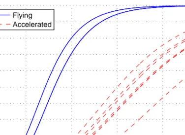
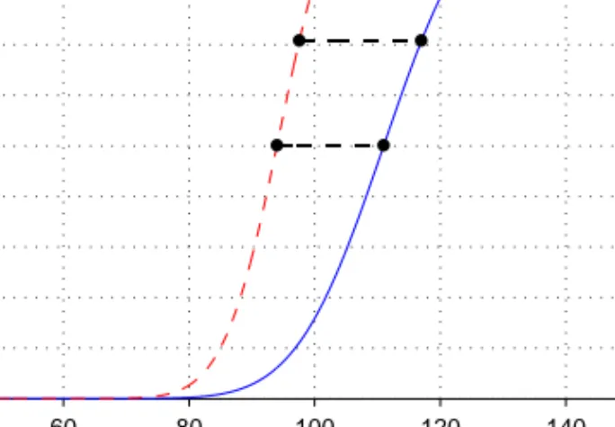
generally more willing to accept a gap limited by a natural vision obstruction than similar gaps limited by oncoming vehicles. Using these descriptors, the probability of accepting a certain overtaking gap does not only depend on the length of the gap but also on the other descriptors. This leads to one probability function for each combination of descriptors. Quite a large data bank is required to estimate all these functions. Some studies and estimations of the overtaking probability have been conducted, see McLean (1989) for an overview. Figure 2.10 shows examples of probability functions for overtaking situations with an oncoming vehicle in sight. The functions are estimations for Swedish roads which are presented in Carlsson (1993). As can be seen in the figure, the overtaking probability for a flying overtaking was estimated to be higher than the probability for an accelerated overtaking with the same available gap.

0 200 400 600 800 1000 0 0.1 0.2 0.3 0.4 0.5 0.6 0.7 0.8 0.9 1

Distance to oncoming vehicle, [m] Flying

Accelerated

Figure 2.10: Probability functions for overtaking decisions, combinations of descriptors with oncoming vehicle in sight, (Carlsson, 1993).

2.3.4 Speed adaptation models

Most traffic simulation models use some desired speed parameter to de-scribe drivers’ preferred driving speed. Generally, a normal distribution

is used to model the variation in desired speed among drivers. However, a driver’s desired speed is not constant. The desired speed varies depend-ing on the current road design. On urban roads or freeways, a driver’s desired speed mainly depends on the speed limit. However, on rural roads, like two-lane highways, the desired speed also varies with road width and horizontal curvature for example. To model that a driver’s desired speed varies depending on the road design, some kind of speed adaptation model is required.

One possible modeling approach for roads where the speed limit is the only or the main determining factor of the desired speed is to assign each driver a desired speed for each possible speed limit. This gives a flexible model which can catch the variation in desired speed with regard to speed limits. A similar but little less flexible way, is to define a relative desired speed distribution. A driver’s desired speed is then calculated by adding the assigned relative speed to the speed limit. This approach was used by Yang (1997) and Ahmed (1999) for example. In Barcel´o and Casas (2002) a similar approach was used, whereby drivers’ desired speeds were deduced by multiplying the speed limit with an individual speed acceptance parameter. The speed acceptance parameter follows a normal distribution among drivers.

On rural roads, drivers’ desired speed is also affected by the road geometry. In addition to the speed limit, the desired speed can for in-stance depend on the road width and the horizontal curvature. Brodin and Carlsson (1986) include a presentation of a speed adaptation model in which a driver’s desired speed is affected by the speed limit, the road width, and the horizontal curvature. In this model, each driver is as-signed a basic desired speed, which is adjusted to a desired speed for each road section. This is done by reducing the median speed according to three sub-models, one for each of the above mentioned factors. How-ever, in this model, a driver’s desired speed is not only the result of a shift of the distribution curve, which is the case in the models by Yang (1997), Ahmed (1999), and Barcel´o and Casas (2002). In the model by Brodin and Carlsson (1986), the desired speed distribution curve is also rotated around its median, see the example in Figure 2.11. This makes it possible to tune the model in such a way that drivers with high desired speeds are more affected by a speed limit than drivers with low desired speeds. How much the curve is rotated depends on the factors that addressed the reduction. Different rotation parameters are used for adaptation caused by the road width, the speed limit, and the horizontal

curvature. 40 60 80 100 120 140 160 0 0.1 0.2 0.3 0.4 0.5 0.6 0.7 0.8 0.9 1

Cumulative desired speed distributions

Desired speed, [km/h] Basic desired speed

Speed limit 90

simulators

It is well known that the surrounding road and traffic environment in-fluences drivers and their behavior. For example, the road environment affects drivers’ desired speed, lateral positioning, and overtaking behav-ior. Another main influence factor is of course other road users. Other vehicles certainly affect a driver’s travel speed and travel time, but they also influence a driver’s awareness. In order to be a valid representation of real driving, driving simulators need to present a realistic visualiza-tion of the driver’s environment. Thus, the road and traffic environment should affect drivers in the same way as in reality. Realism is a quite abstract word and it is not obvious what is meant with a realistic simu-lation of vehicles. In Bailey et al. (1999) and later in Wright (2000) the following requirements for a realistic traffic behavior are outlined:

• Intelligence: The individual vehicles must be able to drive through a network in a way corresponding to a possible human being.

• Unpredictability: The simulated traffic should be able to mimic the unpredictability of real traffic, e. g. dealing with the variation in driver behavior among drivers and also over time for a specific driver.

• Virtual personalities: This third category can be seen as a further specification of the unpredictability requirement. Wright (2000) suggests that a realistic traffic environment should include various driver types such as normal, fatigued, aggressive and drunk. Excluding the requirement on virtual personalities, a microscopic traffic simulation model should be able to reproduce realistic driver behavior including the variation in driver behavior both among drivers and over time for a specific driver. This implies not only intelligence and un-predictability but also unintelligence and un-predictability. It is equally important that the simulator drivers feel that they can predict other

drivers’ actions to the same extent as in reality and that other drivers act unintelligently to the same extent as in reality. In the end, it is important that the driving simulator and its sub-models induce realis-tic subject driving behavior at operational, tacrealis-tical and strategical level (using the definitions of operational, tactical, and strategical level pre-sented in Michon (1985)).

The need for a realistic representation of the traffic environment sometimes stands in contradiction to the design of useful driving simu-lator experiments. To gain a deeper understanding of the background to this dilemma, this chapter starts with a presentation of driving simu-lator experiments and scenarios. Differences between traditional appli-cations of traffic simulation and this application is discussed in Section 3.2. Section 3.3 includes a survey of common modeling approaches for the simulation of surrounding vehicles in driving simulators.

3.1

Driving simulator experiments

Driving simulators offer the possibility to conduct many different kinds of experiments. One of the strengths of driving simulator experiments is the possibility they provide to study situations or conditions that rarely occur in reality. It is also possible to study situations or conditions that are too risky or un-ethical to study in real traffic, for example fatigue or drunk drivers. Another strength is the possibility they provide for sys-tematic variation of test parameters in order to distinguish differences or correlations between different variables. A driving simulator experiment is specified through an experimental design which may involve one or several scenarios which in turn, may contain one or several events.

3.1.1 Scenarios, events and experimental designs

A driving simulator scenario is a specification of the road and traffic environment along the road. This includes a specification of the road environment e. g. specification of road geometry, road surface, weather conditions, and surroundings such as trees and houses. A scenario must also include a specification of other road users and their actions. A scenario can be seen as a constellation of consecutive traffic situations or events, which starts when a certain condition is met and ends when another condition is met, (van Wolffelaar, 1999), or following the termi-nology used in Alloyer et al. (1997), a constellation of scenes. Alloyer

et al. (1997) define a scene as a specification of: the area in which the scene will take place, which actors will be present, what is going to happen, and in which order things are going to happen.

Predefined events are often used in order to conduct accelerated test-ing. Some traffic situations or events occur seldom, and many simulator hours are thus required to study drivers’ behavior in such situations if we should wait until they arise by themselves. One of the strengths of driving simulators is that it is possible to shorten the time between these situations. An example of an event, taken from Bolling et al. (2004), is a situation in which a bus is standing at a bus stop in a low complexity urban environment. Four seconds before the simulator driver reaches the bus stop, the bus switches on its left indicator and starts to pull out into the main road. When approaching the bus stop, the driver meets a quite high oncoming traffic flow, which makes it difficult to overtake the bus. If the driver does not yield for the bus, the bus will remain at the bus stop. But if the driver yields for the bus, the bus will accelerate up to a speed of 50 km/h and then stops at the next bus stop. During the drive to the next bus stop, oncoming traffic flow is kept at a high level in order to prevent the subject from overtaking. To sum up, a scenario is a specification of the road environment and a number of events, including information about when and where the events will take place.

The experimental design for a driving simulator experiment includes the specification of how many participants should be involved in the experiment and which scenarios they should drive. The experimental design also includes the specification of which independent variables to use. The independent variables can for example be an Advanced Driver Assistance System (ADAS), the friction on the road, or road type. It is also necessary to specify how the independent variables should be varied among the participants. One possibility is to use a between group design, in which an independent variable is varied between different groups of participants. A possible between group design for the study of an ADAS is to let half of the participants drive with an ADAS letting the other half be a control group, i. e. driving the same scenario without the ADAS. Another possibility is to use a within group design, which implies that all participants drive under all premises, for example both with and without an ADAS. It is also possible to use mixed designs, for example a between group design for one independent variable and a within group design for another independent variable.