Thesis for the Degree of Master of Science in Engineering physics
Exploratory statistical study of long-term variability in
echocardiographic indices (echocardiovariability) in
healthy and diseased
Amanda Albano
February 10, 2013
Department of Physics Umeå institute of technology
Umeå University Umeå, Sweden
Exploratory statistical study of long-term variability in
echocardiographic indices (echocardiovariability) in
healthy and diseased
Amanda Albano February 10, 2013
Master Thesis
Department of Physics Umeå University
Supervisor: Christer Grönlund, Medicinsk Teknik FoU, CMTS
Examiner: Jun Yu, Department of Mathematics and Mathemathical Statistics
This thesis has been prepared using X E LATEX
Copyright ©Amanda Albano, 2013. All rights reserved
Department of Physics Umeå institute of technology Umeå University
SE-901 87 Umeå, Sweden Phone: +46(0)90 785 69 13
Author e-mail: amanda.lm.albano@gmail.com
Abstract
Exploratory statistical study of long-term variability in
echocardio-graphic indices (echocardiovariability) in healthy and diseased
Heart rate variability, HRV, has been well researched for some decades. The oscillations of the heart rate is studied over a time period of some minutes up to 24 hours, it is measured with electrocardiography, ECG. From this one has concluded that the heart rate signal oscillates in accordance with the respiration, the resistance in the vessels etc.
The most frequently used examination method of the heart is done with ultrasound, called echocardiography. One interesting variable at a time is measured and it is measured for a single heartbeat. With inspiration of the HRV studies this project focuses on some of the variables measured with ultrasound but over time and simultaneously. The variables of interest are the myocardial motion and the blood flow in the left part of the heart, they are measured over two minutes. To complement these variables the well known variables HR and Resp are measured with ECG and added to the analysis.
The methods used for analysing the variables are first of all descriptive statistics like mean and standard deviation. Secondly spectral analysis is performed to investigate in which frequencies the variables oscillates. Through coherence this is compared with the spectrum for HR where the three peaks have known origin. Finally principal component analysis, PCA, is performed as a method to compare all variables at the same time.
The analyses are performed on seven measurements from five (5) healthy persons and five measurements from four (4) patients with the disease FAP (“Skelleftesjukan”). The variables are investigated and described for the healthy persons first, then the healthy persons and patients are compared.
The result from the study shows that most of the echo-variables oscillate in accordance with the respiration and the heart rate. For a healthy person the oscillations are within normal values and the relative deviation is around 10%. The patients with FAP are most affected in the variables connected to the myocardium apart from HR, which is known since before.
The coherence between the echo-variables and HR is low in one of VLF, very low frequency, or LF, low frequency, region and high in the other. In HF, high frequency, region the coherence is high for all variables.
Finally the PCA was conducted on measurements from all healthy persons as one data set, from one of the healthy persons and from one of the patients with FAP. The analysis showed that for healthy persons respiration is the process causing most variation and all of the echo-variables have a correlation to the respiration. For a patient with FAP the respiration is not as salient. A PCA over blocks of data at different
time points however show that the signals are not oscillating in the same way multivariately over the whole time series.
Sammanfattning
Explorativa statistiska långtidsstudier av variabiliteten i
ekokardio-grafiska index (ekokardiovariabilitet) hos friska och sjuka
Hjärtfrekvensvariabilitet, HRV, är ett väl utforskat område sedan några årtionden tillbaka. Svängningarna i hjärtfrekvensen studeras över tidsperioder av några minuter upp till 24 timmar och mäts med elektrokardio-grafi, EKG. Från det har man kunnat sluta sig till att signalen för hjärtfrekvensen oscillerar enligt signalen för andningen, kärlresistans etc.
Den mest använda undersökningsmetoden på hjärtat utförs med ultraljud, ekokardiografi. De intressanta variablerna mäts en i taget och för ett hjärtslag åt gången. Med inspiration från studierna av HRV fokuserar det här projektet på några av variablerna som mäts med ultraljud, men som tidsserier och simultant mätta. De intressanta variablerna är tagna från hjärtmuskeln och blodflödet i den vänstra delen av hjärtat. Mätningarna görs över två minuter. För att komplettera dessa variabler mäts de välkända variablerna HR och Resp med EKG och läggs till analysen.
Metoderna för att analysera datat är först av allt beskrivande statistik, såsom medelvärde och standard-avvikelse. I ett andra steg görs en spektralanalys för att undersöka inom vilka frekvenser signalerna oscillerar. Genom koherens jämförs detta med spektrum för HR där de tre topparna har känt ursprung. Slutligen utförs en principalkomponentanalys, PCA, som en metod för att jämföra alla variabler samtidigt.
Analyserna utförs på sju mätninger från fem (5) friska personer och fem mätningar från fyra (4) patienter med FAP (“Skelleftesjukan”). Variablerna undersöks och beskrivs först för de friska personerna, sedan jämförs de friska och sjuka personerna.
Resultatet av studien visar att största delen av eko-variablerna oscillerar i enighet med andningen och hjärt-frekvensen. För en frisk person är svängningarna inom normala värden och den relativa avvikelsen är ungefär 10%. För patienterna med FAP påverkas framförallt variablerna kopplade till hjärtmuskeln förutom HR som man visste sedan tidigare.
Koherensen mellan eko-variablerna och HR är låg i antingen VLF-, very low frequency, eller LF-, low fre-quency, området och hög i den andra. I HF-, high frefre-quency, området är koherensen hög för alla variabler.
Slutligen görs PCA på mätningarna från alla friska personer som ett dataset, på en av de friska personerna och på en av patienterna med FAP. Analysen visar att för friska personer är andningen den process som orsakar mest variation och alla eko-variabler har en korrelation till andningen. För en patient med FAP är andningen inte lika framträdande. En PCA av block ur datat vid olika tidpunkter i signalen visar dock att signalerna inte svänger multivariat på samma sätt genom hela tidsserien.
Contents
Chapter 1 – Introduction 1 1.1 Background . . . 1 1.2 Purpose . . . 1 1.3 Goals . . . 2 1.4 Expected results . . . 2 Chapter 2 – Theory 3 2.1 HRV - Heart rate variability . . . 32.2 Heart anatomy and physiology . . . 5
2.2.1 Diastole in the left heart . . . 5
2.3 FAP - Familial Amyloidotic Polyneuropathy . . . 7
2.4 ECG - Electrocardiogram . . . 7
2.5 Ultrasound . . . 7
2.5.1 Medical ultrasound - ultra sonography . . . 8
2.5.2 Echocardiography . . . 8
Chapter 3 – Material and methods 11 3.1 Data . . . 11 3.1.1 Measurements . . . 12 3.1.2 Variables . . . 12 3.2 Dataprocessing . . . 13 3.2.1 Missing values . . . 13 3.2.2 Outliers . . . 14 iii
3.2.3 Evenly spaced time series . . . 14 3.3 Limitations . . . 14 3.4 Univariate analysis . . . 15 3.4.1 Stationarity . . . 15 3.4.2 Spectral analysis . . . 16 3.5 Multivariate analysis . . . 17 3.5.1 Spectral analysis . . . 17
3.5.2 PCA - Principal Component Analysis . . . 18
3.6 Comparison between healthy and FAP . . . 22
Chapter 4 – Results and Discussion 25 4.1 Univariate analysis . . . 25 4.1.1 Signals . . . 25 4.1.2 Stationarity . . . 27 4.1.3 Descriptive statistics . . . 28 4.1.4 Spectra . . . 31 4.2 Multivariate analysis . . . 33 4.2.1 Spectral analysis . . . 33 4.2.2 PCA . . . 40 Chapter 5 – Conclusions 49 5.1 Univariate analysis . . . 49 5.2 Multivariate analysis . . . 50 5.2.1 Development of PCA . . . 50 5.3 Continuance . . . 51 References 53 iv
Appendix 55
A Descriptive statistics . . . 55
A.1 Healthy persons . . . 55
A.2 Patients with FAP . . . 57
B Coherence . . . 59
C PCA . . . 63
C.1 Frequency regions . . . 63
Chapter 1
Introduction
1.1
Background
Since the 60’s heart rate variability, HRV, has been subject for research [18]. That is, investigating how the heart rate varies if it is measured continuously over time, some minutes up to 24h. By this it has been discovered that the heart rate is oscillating in accordance with the respiration in a healthy person. Even more important is that by looking at the HRV the function of the autonomous nervous system can be investigated.
The heart rate is measured with electrocardiography, ECG, but today the most commonly used examination method of heart function is ecocardiography, ultrasound of the heart [11]. In these examinations each variable must be measured separately and this can only be done for one heart beat at a time, not several subsequent. For example the velocity of the blood flow can be measured but not at the same time as the velocity of the myocardium, this gives a value only for the current heart beat not for several subsequent heart beats. Inspired by the research of HRV this project’s idea is to investigate how the measured variables from ecocardiography behaves when measured as a continuous time series, as well as simultaneously.
1.2
Purpose
The project aims to study variations in longer sequences of the variables and indices measured by echocar-diography, echo-variables. Our vision is that this can increase the understanding of how a healthy heart function in resting phase.
The echocardiographical measurements is hence the project core. We want to use this for exploration of the variables themselves but also the interaction among them and with respiration, Resp., and heart rate, HR.
2 Introduction
1.3
Goals
The specic goals with this thesis are presented below in the order of priority:
1. Make an inventory of and chose interesting variables
2. Describe the chosen variable’s variation univariate
3. Study variations and oscillations that are connected to HR and Resp.
4. Study variations and oscillations that are not connected to HR and Resp.
5. Describe dependencies, interactions and covariation amongst the variables, multivariate
6. Compare healthy persons with patients known to have a specific heart problem, FAP
1.4
Expected results
From what is known from previous work the following are expected results due to the physiology involving the heart and lungs.
1. The respiration should be visible in all variables since respiration is the main reason of pressure changes in the chest as well as of heart rate variability
2. The same mechanisms that give low frequency variability in HR will show in all or at least some of the echo-variables as well
Chapter 2
Theory
2.1
HRV - Heart rate variability
The research on HRV has concluded that several oscillating processes influence the HR and how it is os-cillating. In Figure 2.1 is an example of how the heart rate varies, underneath is a simultaneously measured respiratory signal.
What we can see is the heart rate oscillating in accordance with the respiration. Apart from the obvious we can also see a slower oscillation, in fact it is two slow oscillations. This is visible if a spectrum of this HR signal is viewed, see Figure 2.2.
From this research has concluded that the highest frequency is the respiratory process. The second peak is called LF, low frequency, and it is a process of the musculature of the vessel wall that causes the oscillation. Finally the lowest visible peak in this spectra is called VLF, very low frequency, and the cause is neurogenic process in the vessel wall. The peak in the LF region is usually situated around 0.1Hz and the peak in the VLF region around 0.04Hz. [13]
4 Theory
Figure 2.1: Heart rate variations with simultaneous breathing
2.2. Heart anatomy and physiology 5
2.2
Heart anatomy and physiology
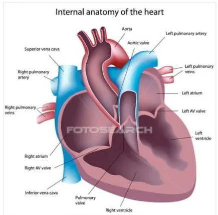
In Figure 2.3 is a schematic cross section of the heart.
Figure 2.3: A cut through of the heart showing the atria and ventricles positioning.
The heart consist of four chambers, two atrium and two ventricles which are separated in a right and left part with one of each chamber in both parts. The passages between the chambers and from the ventricles to the vessels have valves which closes and opens depending on which way the blood should flow. The walls of the heart, the heart muscle, is called myocardium. [15]
2.2.1 Diastole in the left heart
Diastole is the phase when the heart relaxes and the ventricles are filled with blood. For the left side of the heart the phase is separated into early and late diastole (atrial systole). In early diastole the myocardium of the ventricle is relaxed and since the pressure in the blood filled atrium is higher than in the empty ventricle the mitral valve opens. Due to the lower pressure and relaxation of the myocardium a suction towards the ventricle occurs which creates a high blood flow from atrium to ventricle. About 80% of the blood flows passively like this, although as more blood enters the ventricle the pressure evens out and finally an electric
6 Theory
impulse causes the atrial kick or atrial systole. Then the atrium is contracted to push the remaining 20% of blood into the ventricle. [15]
During early diastole, when a force of pressure gradient and suction is dominating, in a healthy heart the peak velocity of the myocardial motion occurs just before the peak velocity of the blood flow. The two quantities are labelled as E and Em(or E’), where E stands for early and the index m (or ’) for myocardium.
During the latter part of diastole, atrial systole, when the mechanical contraction of the atrium is the domi-nating force, there are as well a peak velocity of the blood flow and myocardial motion although not as high as the early diastole peak velocities. These are called A and Amrespectively.
The two velocity curves can be seen in Figure 2.4.
2.3. FAP - Familial Amyloidotic Polyneuropathy 7
2.3
FAP - Familial Amyloidotic Polyneuropathy
One part of this project is to compare healthy persons with patients. In particular the patients disease is FAP, familial amyloidotic polyneuropathy. It is a hereditary disease which is rare but exists all over the world although it is more common in northern Sweden (Norr- and Västerbotten), Portugal, Brazil and Japan. In Sweden it is known as “Skelleftesjukan”.
A consequence of the disease is rhythm disturbances of the heart rate. The cause of this is too much amyloidosis around the nerves which makes the autonomous nervous system loosing its capability to regulate the heart rate. Also remaining amyloidosis in the myocardium make the muscle stiff and the pumping ability impaired. Viewing the HR-signal from a FAP-patients reveals that they have very small variations and the respiration causes almost no variation at all. [6]
One of the problems with decreased pumping ability is an increased filling pressure in the left ventricle. The filling pressure is estimated non-invasively through the variables measured with ecocardiography during diastole, because of that these patients are interesting in this project. They are also interesting because of their lack of variation in heart rate due to the impaired function of the nervous system to regulate it.
2.4
ECG - Electrocardiogram
With the electrocardiogram the electric activity in the heart is measured. This can be used to identify different stages in the heart cycle and there the strongest electrical impulse occur at systole, when the ventricles are emptied. That peak is called R-peak and therefore the length of a heart beat is named RR-interval. If the RR-interval is inverted and multiplied with 60 the instant beat per minutes, or heart rate HR, is achieved. [15]
2.5
Ultrasound
Sound propagates as a longitudinal wave, that means it is not a wave as can be seen on the ocean but condensations and rarefactions of e.g. air. Every material has specific properties such as density which make the sound propagate differently in different materials. For example the speed of sound in air is about 343.2m/s but in water it is about 1484m/s.
At intersections between materials some of the sound will be reflected and heading back to the source and the remaining part will be transmitted through the new material. Also some of the energy in the sound wave will be lost by absorption in the materials, hence the materials are draining the sound wave of its energy.
Ultrasound are all sound waves above a frequency of 20kHz, as a reference humans can hear about 20-20000(20k)Hz.
8 Theory
2.5.1 Medical ultrasound - ultra sonography
Medical ultrasound is based on the reflection and transmission occurring at tissue intersections. An ultra-sound wave is sent in to the body and the echoes coming back from tissue intersections are recorded and imaged. More about the imaging can be read in Persson (2001) [11].
The devices used in clinical application has a piezoelectric crystal which is stimulated by an electric signal to start vibrating. The vibrations causes an ultrasound wave and one uses frequencies above 1MHz in clinical application. To get a 2D view a probe containing a 1D array of piezoelectric crystals creates ultrasound waves in several columns which build up a 2D image. [11]
2.5.2 Echocardiography
Ecocardiography is ultrasound of the heart, cardio, and one uses frequencies around 3MHz for cardiac imaging. It is used for many purposes, it can measure volume and thickness of the heart, reveal erroneous blood flow or malfunctioning valves etc. Also by using for instance the Doppler effect velocities of blood and myocardium can be measured.
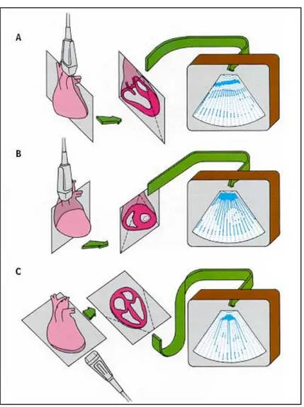
Depending on the purpose of the measurment the probe can be tilted to different angles to achieve different cross-sections, see Figure 2.5. [11]
2.5. Ultrasound 9
Chapter 3
Material and methods
The study focuses on studying the diastolic phase of the left heart in healthy persons and patients with FAP. First the variables are studied univariately, one at a time, to describe their behaviour and variations. Secondly they are studied multivariate, several at a time, to compare their behaviour and variations. The multivariate study is divided to compare first the echo-variables with HR and Resp. and then comparing all the variables at the same time. By this we try to accomplish an easily followed progression in the methods and results.
3.1
Data
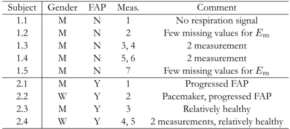
The data consists of seven (7) measurements on five (5) healthy persons, and five (5) measurements on four (4) patients with FAP. The healthy persons are age 28 to 38 and the patients with FAP 45 to 55. In Table 3.1 is information of the different persons.
Table 3.1: Data for the persons involved as subjects in the project
Subject Gender FAP Meas. Comment
1.1 M N 1 No respiration signal
1.2 M N 2 Few missing values for Em
1.3 M N 3, 4 2 measurement
1.4 M N 5, 6 2 measurement
1.5 M N 7 Few missing values for Em
2.1 M Y 1 Progressed FAP
2.2 W Y 2 Pacemaker, progressed FAP
2.3 M Y 3 Relatively healthy
2.4 W Y 4, 5 2 measurements, relatively healthy
12 Material and methods
3.1.1 Measurements
The measurements were performed with +Vivid E9 GE Vingmed with cardiac phased array probe tilted to get a view from the apical position, C in Figure 2.5. Simultaneously the electrical activity of the heart and the respiration is measured with electrodes, ECG. The measurements are approximately 120 seconds in duration and the time points when each heart beat occurs is saved together with the electrical measurements.
The person subject for a measurement lies down and is still during the whole measurement. Before the measurement he or she have been resting to stabilize their pulse. Two of the healthy persons and one of the patients with FAP are measured two times to compare if a measurement on one person can be repeated with similar results.
3.1.2 Variables
The variables comes from the blood flow and myocardial motion during diastole. Possible variables are discussed with cardiologist Per Lindqvist and the final choice can be seen in Table 3.2.
Table 3.2: Variables used in analysis Variable Unit Description
E cm/s Early peak velocity of blood flow
A cm/s Late (Atrial) peak velocity of blood flow
Em cm/s Early peak velocity of left ventricular
my-ocardium
Am cm/s Late (Atrial) peak velocity of left ventricular
my-ocardium
E/A - Ratio used for assessing the blood flow
E/Em - Ratio used for assessing the filling pressure
∆tE ms Difference in time between early peak velocities
∆tRRE ms Difference in time between heart beat and early
blood peak
∆tRREm ms Difference in time between heart beat and early
myocardial peak
∆tA ms Difference in time between late peak velocities
In Figure 3.1 is the heart with marked positions to the left and the profile of the curves from the measurement points marked with the interesting variables to the right.
For a more thoroughly description of cardiac physiology see Section 2.2. The variables were chosen to have clinical importance as well as being easy to measure although the two variables ∆tRRE and ∆tRREm are
only considered as variables for comparison between healthy and FAP-patients univariately. The variables most used in clinical assessment is E/Emwhich is used for assessing the filling pressure in the left ventricle.
3.2. Dataprocessing 13
(a) Where the different variables are measured
(b)The velocity curves of blood and myocardium
Figure 3.1: Points and curves of measurement
Both the A and Ampeak shows up in the same curve as E and Emrespectively and therefore they are taken
into the analysis as well although they are seldom used in clinic. The two time differences, ∆tEand ∆tA, are
more used in research than in clinical application but the prior might as well be a indicator of filling pressure [8], similarly to E/Em.
3.2
Dataprocessing
For the above variables some preprocessing of the signals are made before further analysis. Since the two ratios are built up of other variables the preprocessing is made on the single variables before combining them to ratios.
3.2.1 Missing values
Missing values occurs in all of the interesting variables. They are removed and new values at the same time points are interpolated with cubic splines. A cubic spline is a third order polynomial, eq. 3.1, defined on a specific interval. When using cubic splines for interpolation third order polynomials are defined at time intervals where there are missing values. Each of these splines are created under the restriction that they should be continuous up to second derivative at the end points which combine the spline with the non-missing values. [4]
y = a0+ a1x + a2x2+ a3x3 (3.1)
If there are any missing values in the beginning or end of any of the variables the series of signals are shortened to avoid extrapolation.
14 Material and methods
A point out is that for the healthy persons four of the measurements have almost 50% missing values in the variables Em, E/Em, ∆tEand ∆tRREmwhich can be a problem for the estimation of spectra. The fastest
oscillation, respiration, is for example hard to catch for those measurements.
3.2.2 Outliers
After missing values are taken care of outliers are removed. They can be removed straight away since bio-logical heart arrhythmia can occur, even in normal persons, and that is not what is intended to explain in this study. The other error that can occur is due to bad measurements which also should be taken away since it is not the true process. To avoid any distribution assumptions a non-parametric method is used. Tukey’s rule is a non-parametric method for identifying outlying and extreme observations, described in eq. 3.2. Any observations outside that interval is concerned as a outlying observation.
[Q1− d · iqr Q3+ d· iqr] (3.2)
iqr = Q3− Q1 (3.3)
Here Q1and Q3are the lower and upper empirical quartile respectively, d a proper constant and iqr, eq. 3.3,
is the inter quartile range which is the distance between Q1and Q3. The constant d is usually set to 1.5 or 3
and the two distances are called inner and outer fences where observations between the fences are counted as outliers and observations outside the second fence is counted as extreme. [5]
In this study extreme observations outside
[Q1− 3 · iqr Q3+ 3· iqr]
are removed, hence with d = 3.
3.2.3 Evenly spaced time series
Most of the methods used for analysing time series or signals, like spectral analysis, assume an evenly spaced sampling, hence that the time interval between two consecutive measured values is the same through the series. This data is sampled unevenly since the measurements of all variables are related to a heart beat and the time for a heart beat is registered as it occurs. To achieve an evenly spaced time series interpolation with cubic splines is performed. To get smoother and foremost evenly spaced time series all signals are interpolated to sample rate 4Hz, a sample rate used in HRV application [18].
3.3
Limitations
In this study the limitations are mainly in the data. First of all the data comes from two small groups of subjects with similar properties which makes it hard to draw general conclusions. Secondly the patients with FAP is a heterogeneous group regarding their disease, the first patient has a progressed disease, the second have a pacemaker and the other two have not such a progressed disease. Finally the measurements of the tissue velocity on healthy persons had poor quality in all but measurement 2 and 7 meaning that there were many missing values that needed to be interpolated.
3.4. Univariate analysis 15
3.4
Univariate analysis
Looking at the signals plotted against time is the first step of the analysis. From there descriptive statistic is produced to get quantitative measurements of the signals. The parameters derived from the samples are presented in Table 3.3.
Table 3.3: Interesting parameters for descriptive statistics Parameter Explanation Calculation
ˆ µ = ¯x Sample mean n1 n ∑ i=1 xi ˆ
σ = s Sample standard de-viation √ 1 n−1 n ∑ i=1 (xi− ¯x)2 ˆ cv = σµˆˆ Sample coefficient of variation s ¯ x 3.4.1 Stationarity
Stationarity is often a prerequisite for analysis of time series. It means that the mean of the time series, or signal, should not drift or change and that the variance should be the same all the way.
This is tested using Kwiatkowski–Phillips–Schmidt–Shin, KPSS, test which is a test for stationarity around a deterministic trend. In eq. 3.4 the processes used for testing is presented and explained. Below is the hypothesis which are tested by the KPSS test.
yt = ct+ δt + ut (3.4)
ct = ct−1+ vt (3.5)
In eq. 3.4 the variable utis a stationary process and δt a linear trend with slope δ. The process ctdescribed
in eq. 3.5 is a random walk where vt∼ IID(0, σ2). The KPSS test uses the hypothesis
H0 : σ2 = 0
against
H1 : σ2> 0.
If H0 is true the random walk ct will just be a constant intercept in the process yt. If however H1 is
true the process ctwill be a random walk with a unit root and hence the process ytwould contain a unit
root and not be stationary. The numeric calculation of the p-value for testing the hypothesis is limited to 0.010 < p < 0.100. [14]
If there is not a stationary trend in the data it is taken care of through subtracting the best linear fit from the data, called de-trending. It is necessary to have a stationary time series when for example calculating the power spectrum of a variable.
16 Material and methods
3.4.2 Spectral analysis
Spectral analysis is used to analyse in which frequency domains the variation of a signal is dominating. The power in each frequency is calculated based on fourier transform of the signal [9]. In this first exploration of the variables we prefer to use non-parametric methods as much as possible and therefore chooses fourier transform.
A spectrum is created by calculating the power in each frequency, hence the spectrum of a signal is called Power Spectral Density, PSD. In eq. 3.6 is how the average power for signal{xt} over an interval t =
1, . . . , n is defined. Pxx = 1 n n ∑ k=1 |xk|2 (3.6)
Calculation of the power of a signal in each frequency component is done by represent the signal in frequency domain using fourier series representation of the signal,{xt}t=1...n. The signal is represented as a series of
sine and cosine, which can be written in complex form as in eq. 3.7 where f = kn. The coefficients ckcan
then be written as in eq. 3.8, and from this the power of each frequency component is calculated as in eq. 3.9. [9] xt = n ∑ k=1 ckei2πkt/n (3.7) ck = 1 n n ∑ t=1 xte−i2πkt/n (3.8) Pxx(f ) = |ck|2 (3.9)
Fourier series representation of a signal is a special case of fourier transform which is a method used to convert the representation of a signal between time domain and frequency domain. The transform becomes a series when the signal is limited to a specific interval n or is periodic with periodicity n.
To estimate this numerically Welch’s method [17] is used. It is an algorithm where the signal is divided into segments of equal length, then for each segment the signal is windowed and transformed to fourier series representation using the algorithm fast fourier transform. The estimated PSD, eq. 3.10, is calculated based on the numerically estimated coefficients ˆck.
ˆ
Pxx=|ˆck|2 (3.10)
This is called short time fourier transform and the final PSD for the whole signal is calculated as the mean of the segment’s PSD. The segments can be chosen as overlapping to get a more complete representation of the signal. The averaging makes the PSD smoother since only the main frequencies present in every segment will give high peaks. The windowing is used to reduce the effect of non-periodic boundary values. [9]
3.5. Multivariate analysis 17
In this study spectra of the signals are produced using Welch’s method with a hamming window of length one fourth of the signals length, n/4, and overlapping (n/4)/1.05. This is chosen to make the spectra as free from noise as possible but still narrow enough bands to make the strongest peaks visible, mainly the spectra for HR has been used to try this out since it is known to have three clear peaks in its PSD.
Important when analysing the spectra is to have in mind the spectra of the HR and respiratory signal which is produced in the same manner. It is well known that these should contain three and one peak respectively [18].
3.5
Multivariate analysis
The multivariate analysis consists of two parts, first there is a comparison in frequency between each of the echo-variables and the HRV. Second is a PCA performed on all of the variables.
3.5.1 Spectral analysis
The multivariate analysis starts with a visual comparison between the signals PSD’s. It is a qualitative inves-tigation with focus on comparing echo-variables with HR and respiration. From this similarities are derived to a quantitative measure as 1 or 0 depending on if a peak exists in the same frequency as HR or not. The three frequency regions are
VLF: frequencies below 0.05Hz
LF: frequencies around 0.10Hz
HF: frequencies at the respiration frequency, around 0.25 or 0.35Hz
Since qualitative description of the variables similarities and differences is a goal in the study the visualiza-tion of the spectra for comparison is important. This is taken care of by normalizing the spectra with the maximum value, ie. divide every power value with the maximum power. Then all the spectra are plotted from above as surface plots.
One tool for investigating the similarity between two variables in frequency is coherence. It is used to get a feeling of in which frequencies the variables are coherent. Since similar noise also can be coherent it should be verified that there actually is a peak in the PSD at this frequency and not just the same kind of noise.
Coherence, Cxy, is the correlation in frequency domain, hence between the PSD of signal{xt}t=1...n, Pxx,
and signal {yt}t=1...n, Pyy. It uses the information from the cross-PSD, Pxy. In eq. 3.11 is how the
coherence is calculated and in eq. 3.12 is the estimate of Cxy.
Cxy(f ) = |Pxy (f )|2 Pxx(f )Pyy(f ) (3.11) ˆ Cxy(f ) = | ˆ Pxy(f )|2 ˆ Pxx(f ) ˆPyy(f ) (3.12)
18 Material and methods
The notation Pxy is cross power spectral density (CPSD) and it is the PSD of the cross correlation. The
mathematical formula can be seen in eq. 3.13 and the estimator in eq. 3.14.
Pxy(f ) = ∞ ∑ h=−∞ Rxy(h)e−i2πfh (3.13) ˆ Pxy(f ) = ∞ ∑ h=−∞ ˆ Rxy(h)e−i2πfh (3.14)
Cross correlation is the correlation between two time series,{xt} and {yt} based on lag, h. So it is correlation
coefficient between every value in x and yt, for every value of t. The true cross correlation is as in eq. 3.15,
with the cross covariance in eq. 3.16 and the estimator of it in eq. 3.17. The estimator of the cross correlation can finally be seen in eq. 3.18
ρxy(h) = γxy(h) σxσy = √ γxy(h) γxx(0)γyy(0) (3.15) γxy(h) = E((Xt− µX)(Yt+h− µY)) (3.16) ˆ γxy(h) = cxy(h) = 1 n n∑−h t=1 (xt− ¯x)(yt+h− ¯y) if h≥ 0, 1 n n ∑ t=h+1 (xt− ¯x)(yt+h− ¯y) if h < 0, 0 if h >|n| (3.17) ˆ ρxy(h) = rxy(h) = cxy(h) √ cxx(0)cyy(0) (3.18)
In these equations h represents time lag, γxx(h) the auto-covariance function of signal{xt} which at lag 0
is the variance of the signal. The signals are of length n with mean µxand µyrespectively which is estimated
by the sample mean, ¯x and ¯y. [16]
The coherence is calculated using Welch’s method [17] with windowing as in the univariate PSD calculation.
Multiplying the coherence with the PSD is a technique we believe show both where high coherence occur but also if there actually is energy in that frequency instead of just noise. In this project this method is used to investigate the coherence between echo-variables and HR. In the same manner as with the original PSD a quantitative value of the coherence at its highest peak within the HR-frequencies is extracted.
The coherence is also visualized by plotting it together as surface plots. For the multiplication between coherence and PSD a normalization with maximum power is done first.
3.5.2 PCA - Principal Component Analysis
The focus of the spectral analysis is to investigate the relation between the echo-variables and HR. To keep on investigating the relationship between the echo-variables in a similar way would mean many pairwise comparisons which is both time consuming and difficult to get an overview of for interpretation.
3.5. Multivariate analysis 19
A method that consider all variables at the same time is principal component analysis, PCA. It is a multivariate method often used to reduce the dimensionality of data sets with many variables, hence concentrate the information in several variables to a just a few.
Data matrix X consists of n observations and p variables ordered as n× p. The PCA finds the direction in the data with the largest variance and creates a new coordinate axis as a linear combination of the original variables in that direction, the first principal component, PC 1. Next PC is placed in a similar matter but with the condition of being orthogonal to the former and hence uncorrelated with it. This is illustrated in Figure 3.2 with two variables, p = 2 and in equation 3.19-3.20.
Figure 3.2: A scatter plot of two variables can be described by a new coordinate system based on the direction of maximal variance
y1 = pc1 = a11x1+ a12x1 (3.19)
y2 = pc2 = a21x1+ a22x1 (3.20)
The direction of the largest variance is in the direction of the first principal component y1. The direction is
determined by a1= (a11, a12) which is the first eigenvector of the covariance matrix Σ or the correlation
matrix ρ. The following principal components are built up of the following eigenvectors in ascending order. When the original variables are of different magnitude or unit the correlation matrix is used instead of the covariance matrix. All variables are then given equal importance in the analysis. If all variables have the same unit the covariance matrix can be used to capture difference in variance. [7]
The eigenvector aithat constitutes principal component yiconsists of loadings. These loadings are between
-1 and 1 if the correlation matrix is used and shows which of the variables that are important for different directions in the data. If the observed values are put into the equation of each PC new “observations” are created in the tilted coordinate system and they are called scores.
The eigenvalues, λi of each eigenvector, ai, is how much variance each principal component explain.
20 Material and methods each PC as λi p ∑ i=1 λi
and the cumulative variance as
k<p ∑ i=1 λi p ∑ j=1 λj ,
meaning the amount of explained variance for the first k PC’s.
In this study PCA is used to investigate how the variables group in the first components and therefore the loadings are studied. The hope is that such analysis can reveal how the physiologically related variables are grouped with the processes that are related to the respiratory activity and the known processes of HRV. It would also be interesting if the echo-variables show something that are not related to the known processes.
First of all, all the healthy persons are considered as one data set and analysed with
7
∑
meas=1
nmeas
ob-servations in one PCA. Secondly one of the measurements on a healthy person with few missing values, measurement 7, is analysed with PCA. The second analysis is then compared to the first. Also a typical patient with FAP is analysed and the similarities and differences to the PCA made on one healthy person is examined.
The analysis have focus on looking at how the loadings group when plotted for two PC’s against each other, not to interpret the meaning of the principal components. An interpretation of the PC’s would require deep knowledge in physiology and the entire cardiovascular system.
Since the variables units are different the correlation matrix is used to find loadings and eigenvalues. The number of principal components chosen for analysis is based on some thumb rules which are all components with eigenvalue larger than one and/or as many components needed to explain 80% of the total variation [7].
Data processing
The data used in the analysis is the data that has been preprocessed according to the steps in Section 3.2, missing values are removed and new interpolated, outliers are removed and new interpolated and last inter-polation to create an evenly spaced time vector.
The variables included are selected to be ten, namely E, A, Em, Am, ∆tE, ∆tA, HRV LF, HRLF, HRHF
and Resp. The ratios, E/A and E/Em, are excluded since they consists of other variables and the other
two time differences, ∆tRRE and ∆tRREm, were just interesting for the descriptive statistics. The three
variables HRV LF, HRLF and HRHF are the HR signal filtered with bandpass filters to represent the three
different frequency bands in the HR signal. The exact frequency bands are chosen individually for each of the measurements and can be seen in Appendix C. They are filtered like this to make interpretation of the principal components easier.
After all the variables are extracted the data is detrended with a linear trend then centred and scaled, ie. subtraction with mean and division by standard deviation for each variable, see eq. 3.21. This corresponds
3.5. Multivariate analysis 21
to using the correlation matrix in the PCA. [7]
zi =
xi− ¯x
σx
(3.21)
A PCA is then performed on the data and the T2-statistic calculated accordingly to eq. 3.22 where i is observation, ˆyi the vector of scores of all principal components for observation i and the matrix S is the estimated covariance matrix.
Ti2 = ( ˆyi− ¯y)′S−1( ˆyi− ¯y) = = (ˆyi1− ¯y1) 2 λ1 + . . . + (ˆyp1− ¯yp) 2 λp (3.22)
Since the principal components are uncorrelated the final expression is just a sum of squares divided by the eigenvalues, hence the amount of variance. This statistic is commonly used to identify multivariate outlying observations by using that for large samples, > 50 observations, this statistic is approximately χ2-distributed with p degrees of freedom. [7]
In this study the aim is to describe the ordinary process and therefore outlying observations are not of interest and χ2p(α) with α = 0.10 is used as a limit for removing multivariate outliers.
After this a new PCA is performed and the loadings from that analysis is interpreted.
Dependent data
An obstacle for performing a PCA on this data is that the n observation are dependent since they are measured as a time series. It is however not a problem for performing the analysis although the information that lies within the correlation among observations will be lost.
A more thoroughly discussion about possible ways of handling the dependency can be seen in chapter 5.2.
Bootstrap
Bootstrap is a method of re-sampling the sample already obtained to get several estimates of a desired parameter, and hence get a sample of observations for that parameter. The good thing with this is that no distribution assumption for the original sample is needed to get an impression of the distribution for the parameter. [12]
In this study the bootstrap method will be used to calculate confidence intervals for the amount of explained variance and compare this for the different analyses.
An assumption of the bootstrap approach is that the original observations are independent and identically distributed [12]. This mean that the dependence in this data need to be taken care of. The method of resampling observation with blocking has been used previously to take care of this dependence structure [19]. Blocking is that one observation is drawn randomly from the original sample and with it follows the k0 following observations. In this study this is done with replacement, one observation can be drawn several
22 Material and methods
times, and the blocks can be overlapping. The total sample is always of the same size as the original and blocks of k = 20 is used since the dependence in the data is approximately five seconds, which is the slowest respiration period.
From the bootstrapped sample a PCA is performed. The direction of each PC can be both positive and negative, consider Figure 3.2 and if there is any difference with the arrow pointing in any of the directions. To achieve the same direction as the original sample gave, correlation between the bootstrapped PC’s scores and the original PC’s scores is calculated. If the correlation is positive for a PC all loadings keep their sign, but if the correlation is negative the sign is changed for all those loadings. Further the correlation between principal components is calculated since they have similar eigenvalues and therefore PC 1 in the bootstrapped sample can sometimes correspond to PC 2 in the original sample and so forth. If that is the case the bootstrapped PC 1 and 2 are swapped. This is a procedure tried before with good results, [10]. An important remark is that the scores of the original sample need to be re-scrambled in the same way as the re-sampling for the correlation comparison to be correct.
The re-sampling and estimate of loadings is made N = 20000 times and 95% confidence intervals are created according to the basic intervals, see eq. 3.23. [3]
2ˆθn− ˆθ∗0.975< θ < 2ˆθn− ˆθ0.025∗ (3.23)
Here θ is the parameter we desire to estimate and ˆθn is the estimate of θ from the original sample, in
our case the original amount of explained varianc. From the sample created with bootstrap ˆθ0.975∗ is the empirical percentile of the sorted bootstrap sample with 2.5% of the observations above it and ˆθ∗0.025is the corresponding percentile with 2.5% of the data below it.
Verification over time
Since the data are time series a verification is made to see if the PCA give the same result for every segment in time of the signals. A segment length of 25s (in 4Hz signal that is 100 values) is used and a PCA is performed on each of these segments in the same manner as above except for the bootstrap part.
The loadings are then plotted against lag to see how they change depending on where the segment is chosen. This is only done for the PCA performed on one of the healthy person, measurement 7.
3.6
Comparison between healthy and FAP
The same analysis made on the data from healthy persons will be performed on the data from patients with FAP with some minor differences. Thereafter the results are compared to the results from healthy persons.
Focus lies within the univariate analysis and on the descriptive statistics. A Wilcoxon rank-sum test [1] is performed to compare mean values from healthy persons with FAP patients. The samples compared consists of the mean values of all the signals for healthy and patients respectively, the mean values since they are independent which is a prerequisite for the test. This gives 7 observations in the sample for healthy persons and 5 observations in the sample for the patients with FAP. Wilcoxon’s rank-sum test is a non-parametric test and it is used since normality cannot be assumed for the mean values via central limit theorem due to dependent observations [1].
3.6. Comparison between healthy and FAP 23
The Wilcoxon rank-sum test orders each samples observations, of size n = 7 and m = 5, in ascending order. The observations are then numbered according to size, 1 for the smallest and n + m = 12 for the largest. If there is no difference in distribution the sum of the ranks in each sample should not be to extreme. The hypothesises are
H0: The distribution of means for healthy persons and patients with FAP is the same
against
H1 : The distribution of means for FAP patients is shifted
and they are tested with test-statistic as in eq. 3.24.
RF = m=5∑
i=1
R(F )i (3.24)
The test statistic RF is the rank-sum of the ranks, R(F )i , of the observations from the FAP-group (F) since
it is the smaller group. If H0 is correct then the ranks of the observations in the FAP-group could be any
five out of twelve and hence a p-value for the estimated rank, rF, can be calculated as in eq. 3.25. [1]
p = P (RF ≤ rF) =
Number of rank combinations giving R( F ≤ rF
12 5
) (3.25)
This p-value is then compared to the confidence level requested, α, which in this study is set to 0.005, 0.01, 0.05 and 0.1.
The coherence calculation is not performed on FAP-patients since their HR does not have any variations, coherence would then be pointless and probably just show coherence in noise. Instead the qualitative in-spection is about localizing frequency bands where the echo-variables have similar activity not visible in the spectra for HR.
Chapter 4
Results and Discussion
4.1
Univariate analysis
4.1.1 Signals
In Figure 4.1 is an examle of how the signals of the variables can look like for a healthy person. Missing values and outliers are removed and the sampling rate is interpolated to 4Hz.
A first view shows that all of the signals seems to oscillate in accordance with the respiration, which is the signal in the bottom right corner. Also one can notice that the two ratios resembles their denominator more than their numerator. For a healthy person one expect E/Em < 8, 1 < E/A < 3 and ∆tE > 0, which is
fulfilled all the time.
The signals are oscillating just as the heart rate but none of the signals seems to have a trend over time, which they should not when measured on a subject that is lying still.
Figure 4.1 can be compared to a patient with FAP for which the signals looks as in Figure 4.2.
The heart rate looks very different compared to the healthy person, every other heart beat is short and every other is long. This is not noticeable in the echo-variables where however the respiratory oscillations seems to have influence. For the variables E/Em, E/A and ∆tE the values clearly oscillate between both good
and poor according to the boundaries described above.
For the FAP patient the ratio E/Emoscillate between 8 and 13, compared to 4 and 6 for a healthy person.
This means that the value of an important ratio for assessment of this patient oscillate between normal and poor. The same holds for the ratio E/A which oscillate between 0.95 and 1.15 for the patient. The time difference ∆tEis also markedly shorter than for the normal person. This confirm that ∆tE is also affected
in patients with increased filling pressure, apart from E/Emthat was known to be affected since before.
26 Results and Discussion
Figure 4.1: Measurements of all variables for one healthy person
4.1. Univariate analysis 27
4.1.2 Stationarity
The test for stationarity of the signals from the healthy persons give p-values as in Table 4.1 with p-values high enough to not reject H0, stationarity, at any α-level≥ 0.01 marked as bold face.
Table 4.1: Test for stationarity of healthy persons, p-values of KPSS-test
Meas E A Em Am E/A E/Em
1 0.010 0.010 0.010 0.010 0.010 0.010 2 0.010 0.010 0.010 0.010 0.010 0.010 3 0.010 0.010 0.010 0.010 0.010 0.010 4 0.010 0.010 0.010 0.010 0.010 0.010 5 0.010 0.010 0.010 0.010 0.010 0.010 6 0.022 0.010 0.010 0.091 0.010 0.010 7 0.010 0.010 0.010 0.010 0.010 0.010 Meas ∆tE ∆tRRE ∆tRREm ∆tA HR Resp
1 0.010 0.010 0.010 0.010 0.010 NaN 2 0.010 0.010 0.016 0.010 0.010 0.100 3 0.010 0.010 0.010 0.010 0.010 0.100 4 0.010 0.010 0.010 0.010 0.010 0.100 5 0.010 0.010 0.010 0.022 0.010 0.100 6 0.010 0.010 0.010 0.016 0.010 0.100 7 0.010 0.010 0.010 0.010 0.010 0.100
In Table 4.2 are the p-values from the test for the patients with FAP.
Table 4.2: Test for stationarity for patients with FAP, p-values of KPSS-test
Meas E A Em Am E/A E/Em
1 0.050 0.010 0.010 0.083 0.010 0.010
2 0.010 0.011 0.010 0.096 0.010 0.023
3 0.010 0.010 0.010 0.010 0.010 0.010 4 0.010 0.010 0.010 0.010 0.010 0.010 5 0.010 0.010 0.010 0.010 0.023 0.010 Meas ∆tE ∆tRRE ∆tRREm ∆tA HR Resp
1 0.010 0.010 0.010 0.023 0.100 0.100
2 0.010 0.010 0.010 0.010 0.010 0.100
3 0.010 0.010 0.010 0.010 0.010 0.100
4 0.010 0.010 0.010 0.010 0.010 0.100
28 Results and Discussion
The result clearly show that these signals are not stationary except for the respiration. Despite this the analyses described in Chapter 3 are fulfilled but the data is de-trended and the problems of non-stationarity are discussed in concerned tasks.
4.1.3 Descriptive statistics
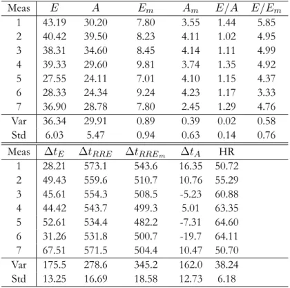
The sample mean of all variables and measurements from the healthy persons are presented in Table 4.3. The variance and standard deviation between the measurements are presented at the bottom of each column.
Table 4.3: Sample mean per variable and measurement for healthy persons
Meas E A Em Am E/A E/Em
1 43.19 30.20 7.80 3.55 1.44 5.85 2 40.42 39.50 8.23 4.11 1.02 4.95 3 38.31 34.60 8.45 4.14 1.11 4.99 4 39.33 29.60 9.81 3.74 1.35 4.92 5 27.55 24.11 7.01 4.10 1.15 4.37 6 28.33 24.34 9.24 4.23 1.17 3.33 7 36.90 28.78 7.80 2.45 1.29 4.76 Var 36.34 29.91 0.89 0.39 0.02 0.58 Std 6.03 5.47 0.94 0.63 0.14 0.76
Meas ∆tE ∆tRRE ∆tRREm ∆tA HR
1 28.21 573.1 543.6 16.35 50.72 2 49.43 559.6 510.7 10.76 55.29 3 45.61 554.3 508.5 -5.23 60.88 4 44.42 543.7 499.3 5.01 63.35 5 52.61 534.4 482.2 -7.31 64.60 6 31.26 531.8 500.7 -19.7 64.11 7 67.51 571.5 504.4 10.47 50.70 Var 175.5 278.6 345.2 162.0 38.24 Std 13.25 16.69 18.58 12.73 6.18
The sample means of the healthy persons are all within normal range but varies a lot between persons. Looking at measurement 3 and 4 as well as 5 and 6, which are person 3 and 4 respectively, we can see that the mean values are for some variables different for a single person but mostly they are very similar.
This should be seen together with the coefficient of variation, cv, which is the standard deviation related to
the mean of each variable and measurement, presented in Table 4.4.
The relative standard deviation seems to be low for all of the variables except for ∆tE and ∆tA. For
4.1. Univariate analysis 29
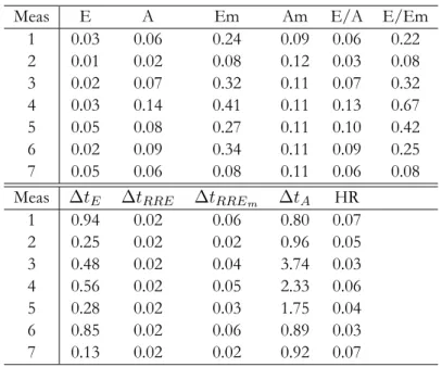
Table 4.4: Coefficient of variation per variable and measurement for healthy persons
Meas E A Em Am E/A E/Em
1 0.03 0.06 0.24 0.09 0.06 0.22 2 0.01 0.02 0.08 0.12 0.03 0.08 3 0.02 0.07 0.32 0.11 0.07 0.32 4 0.03 0.14 0.41 0.11 0.13 0.67 5 0.05 0.08 0.27 0.11 0.10 0.42 6 0.02 0.09 0.34 0.11 0.09 0.25 7 0.05 0.06 0.08 0.11 0.06 0.08
Meas ∆tE ∆tRRE ∆tRREm ∆tA HR
1 0.94 0.02 0.06 0.80 0.07 2 0.25 0.02 0.02 0.96 0.05 3 0.48 0.02 0.04 3.74 0.03 4 0.56 0.02 0.05 2.33 0.06 5 0.28 0.02 0.03 1.75 0.04 6 0.85 0.02 0.06 0.89 0.03 7 0.13 0.02 0.02 0.92 0.07
E/Em, ∆tE and ∆tRREm. For the cv the different measurements on the same person also show that
every measurement does not give the same result for some of the variables.
The mean values of the patients with FAP are presented in the same way as for healthy in Table 4.5.
Table 4.5: Sample mean per variable and measurement for patients with FAP
Meas E A Em Am E/A E/Em
1 29.37 28.55 2.46 3.24 1.03 12.09 2 43.29 36.26 2.22 2.99 1.20 19.59 3 11.44 10.75 5.52 4.57 1.07 2.13 4 11.81 11.16 3.52 6.88 1.06 3.52 5 11.86 11.39 3.39 6.46 1.04 3.60 Var 206.2 143.7 1.70 3.21 0.005 56.19 Std 14.36 11.99 1.30 1.79 0.069 7.50 Meas ∆tE ∆tRRE ∆tRREm ∆tA HR
1 -1.81 514.9 522.8 11.53 72.94 2 -6.50 563.9 570.3 14.78 60.00 3 36.10 535.9 499.9 39.64 61.35 4 38.9 572.8 537.5 38.91 62.11 5 39.68 572.3 536.4 39.27 62.10 Var 543.0 655.4 656.8 206.0 27.44 Std 23.30 25.60 25.63 14.35 5.24
30 Results and Discussion
The first two patients have a more progressed disease than the other two (measurement 4 and 5 is the same patient). There is a clear difference between the first two measurements and the other three, E/Em is at
bad levels (too high) and the mean values of ∆tE is negative for the first two. For the last three this is not
the case however E is much lower than for the healthy persons.
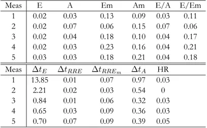
In Table 4.6 is the coefficient of variation for the patients with FAP.
Table 4.6: Coefficient of variation per variable and measurement for patients with FAP
Meas E A Em Am E/A E/Em
1 0.02 0.03 0.13 0.09 0.03 0.11
2 0.02 0.07 0.06 0.15 0.07 0.06
3 0.02 0.04 0.18 0.10 0.04 0.17
4 0.02 0.03 0.23 0.16 0.04 0.21
5 0.03 0.03 0.18 0.21 0.04 0.18
Meas ∆tE ∆tRRE ∆tRREm ∆tA HR
1 13.85 0.01 0.07 0.97 0.03
2 2.21 0.02 0.03 0.54 0
3 0.84 0.01 0.06 0.32 0.03
4 0.65 0.03 0.09 0.36 0.03
5 0.70 0.07 0.09 0.39 0.05
For the first two patients the most noticeable difference, comparing to the healthy persons, is the large variation that ∆tEexperience. Looking at the individual time differences for the E and Empeak, ∆tRRE
and ∆tRREm, the variance in ∆tE may be caused by larger variation in occurance of the myocardial peak
but it is not very clear. The variable ∆tAexperience a decreased variation for the patients relative to the
healthy.
For the patients with FAP there are some clear differences to the healthy persons in mean values. Variables
E and Em seems to have a lower mean for FAP patients than for healthy persons. The ratio E/Em is
markedly higher for the first two measurements and the opposite for the last three. Looking at E and Em
it seems as peak velocity Em has decreased for all patients. For variable E the first two patients does not
seem to be very different from the healthy persons but the last three are much lower, almost a third or a fourth of a healthy persons value. The same pattern shows for A, the late blood peak velocity, as for E. This influence the ratio E/A which is closer to one for the patients with FAP than for the healthy persons.
The time differences ∆tE and ∆tAis clearly different for the FAP patients. The first difference is negative
and the second positive for the first two patients, which was not the case for the healthy persons. For the last three patients ∆tEis still positive but ∆tAis positive as well in opposite to the healthy persons.
By looking at ∆tRREand ∆tRREmfor the patients with FAP one can guess which of the peaks that occurs
earlier or later than for the healthy. It looks as the peak velocity of the myocardium, Em, occurs later rather
4.1. Univariate analysis 31
stiffened heart muscle patients with FAP experiences.
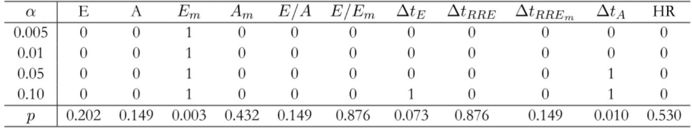
A test for equal mean between the healthy and the patients reveals p-values according to Table 4.7.
Table 4.7: Indication if H0or H1is assumed depending on α-level together with p-values
α E A Em Am E/A E/Em ∆tE ∆tRRE ∆tRREm ∆tA HR
0.005 0 0 1 0 0 0 0 0 0 0 0
0.01 0 0 1 0 0 0 0 0 0 0 0
0.05 0 0 1 0 0 0 0 0 0 1 0
0.10 0 0 1 0 0 0 1 0 0 1 0
p 0.202 0.149 0.003 0.432 0.149 0.876 0.073 0.876 0.149 0.010 0.530
The test for equal means clearly show that Emand ∆tAare different between the two groups. At a
confi-dence level of 90% also ∆tE is significantly different between the two groups. Especially Emand ∆tE are
variables known to be affected for patients with FAP, it is connected to the stiffening of the heart muscle. Important to remember is that the two groups, healthy and patients, are also different age groups and as we grow older we also get a stiffer heart. By this the significant differences in Table 4.7 could be a result of the age difference between the groups instead of the healthy/ill relationship.
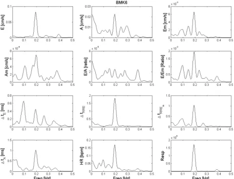
4.1.4 Spectra
In Figure 4.3 are the spectra of all variables for one of the measurements on a healthy person.
Here it is clear that the respiration spectrum is dominated by one peak at 0.2Hz, which is expected and means the breathing has a period of around 5 seconds. The spectrum of the HR-signal has three clear peaks, as should be expected. One for respiration, one in the LF region and one in the VLF region.
For the echo-variables we can see that there is more activity going on, although there is a peak in the same frequency as respiration visible in almost all of the variables. Bare in mind though that due to the signals being non-stationary some of the peaks might only be frequencies present in parts of the signal.
For a patient with FAP the same figure looks as in Figure 4.4.
The HR signal has clearly a different profile. There is neither VLF, LF or HF oscillations in that signal, the only peak occurs because of the “every-other-beat”-profile of this particular patient, Figure 4.2. Looking at the echo-variables reveals that those variables although have energy in all of the normal HR frequencies, however it is not very consistent.
The spectra of the echo-variables shows that the expected processes are present in many of the variables with respiration as the most prominent. Comparing the patients with FAP and the healthy there is not a very big difference in the echo-variables, the difference is mainly in the heart rate.
32 Results and Discussion
Figure 4.3: Spectra of all variables for one of the healthy persons
Since the signals were not stationary an alternative approach would be to use the short time fourier transform but not average over the different segments. Instead it can be used to illustrate how the energy changes over time in the different frequencies. Also there are other methods for estimating the PSD. One alternative would be to base it on an autoregressive, AR, model and hence a transfer function. The advantage is that the peaks would then be exactly at the estimated poles but the disadvantage is that a model order need to be chosen and there will be a problem with the non-stationarity. Further wavelet analysis is also a method one could use for estimating the PSD, in particular as an alternative to short time fourier transform. This was tried in this study but the result was hard to illustrate and present, although it is a strong possible development of the spectral analysis. Read more about different methods used for estimating PSD in HRV application in Wiklund (2001) [18].
4.2. Multivariate analysis 33
Figure 4.4: Spectra of all variables for one of the patients with FAP
4.2
Multivariate analysis
4.2.1 Spectral analysis
The spectra of all the variables for one of the healthy persons are presented in Figure 4.5 as a surface plot. The colours are “Hot and cold” meaning deep red is a high value and dark blue a low value. The lines represent the location of the three peaks in the HR spectrum.
The peaks does not occur at exactly the same places for all of the variables, but it is approximately in the same regions. This may again be an indication of the non-stationarity of the signals, but the frequency of the respiration is clearly a frequency found in all of the variables.
In Figure 4.6 is a summary of in how many measurement a peak is visible divided into the HR regions, each variable is plotted as a separate line. This is created by dividing the spectra for each measurement into three regions based on the HR spectrum (the lines in Figure 4.5) and count for every variable in how many measurement there is a peak for each region.
The spectra in Figure 4.5 shows similarities between the echo-variables and HRV, this is confirmed by the summary in Figure 4.6. However if we look at a measurement where the healthy person’s respiration is at a higher frequency there is more activity between LF and HF peaks in some of the echo-variables than in the HRV, see Figure 4.7.
34 Results and Discussion
Figure 4.5: Spectra of all variables for one of the healthy persons plotted as surfaces (from above) with the variables ordered according to blood and muscle
There seem to be additional processes influencing the echo-variables compared to HR. Further analysis of this should be made, especially since this might be oscillations only present in parts of the signal due to non-stationarity.
In Figure 4.8 is the coherence for each echo-variable with HR as surface plots with the spectrum for HR at the top. Subsequent, in Figure 4.9, is the coherence with HR times the spectrum of each variable illustrated with a surface plot.
The highest coherence in each of the HR regions is presented per variable in Figure 4.10 for one of the measurements.
The pattern shows a possible decline in coherence for the LF region and in general the highest coherence is in the HF region, the region of the respiration frequency. The same figure but for one of the variables, E, and all measurements can be seen in Figure 4.11. The mean coherence for the variable in each region is also presented.
The other variables coherence curves are presented in Appendix B and there is a clear consistent pattern that the coherence is either low in the LF or the VLF region and high in the HF region for all variables. This
4.2. Multivariate analysis 35
Figure 4.6: Number of peaks in the HR frequency regions from the spectra of every measurement
is expected since the respiration should have strong impact on all the variables. The VLF and LF oscillations on the other hand are processes not as salient as the respiration and they might need to be enforced through sudden change in a subjects position for it to really be visible in the PSD [18].
36 Results and Discussion
4.2. Multivariate analysis 37
38 Results and Discussion
4.2. Multivariate analysis 39
Figure 4.10: Coherence at different regions per variable for one of the healthy persons
40 Results and Discussion
4.2.2 PCA
All healthy persons
In Figure 4.12 are the loadings for the first 4 PC’s from the PCA performed on all the healthy persons as one data set.
Figure 4.12: Loadings plotted for two principal components at a time of all healthy persons
The loadings in the first sub figure show what was expected, the respiration and HF oscillations of the heart rate are strongly correlated. Also the blood and myocardial velocities are correlated with the respiration but in different ways. There is one direction with the myocardial velocities and another with the blood velocities and time differences.
PC 2 against 3 does not give much more information than the first plot. In PC 1 against 3 although a division in early and late (ventricular and atrial) velocities can be seen where the atrial velocities pairs with the low frequency oscillations of the heart rate.
4.2. Multivariate analysis 41
The last plot have two clear directions, the blood velocities and HRV LF constitute one and ∆tE and ∆tA
with HRLF the other.
The analysis made on all of the healthy persons show many of the things expected in advance. The respiration is causing the largest variation and we get physiological separation of the variables into blood and myo as well as early and late. One interesting result is that the blood velocities and the time differences show a strong correlation, meaning that the peak velocity of the blood and the inter occurrence time between the peaks are related. If there is a fast blood flow there is also a longer time between the peak velocities.
Important to remember is that this analysis with measurements from different persons only capture the general relations and interactions. There are many other features than these variables that varies between persons, the size of the heart, how well the autonomous nervous system controls HR, myocardial thickness etc.
In Figure 4.13 is the explained variance for the first four principal components, separately and the cumulative variance. It is presented as histograms from the bootstrap sampling with the point estimate from the original sample as a red line and its confidence interval as blue lines.
42 Results and Discussion
The first component explain around 20% of the variation and totally four components explain around 55% of the variation in the data. The low amount of explained variance could be an indicator that there are just as big differences between persons as there are within one persons heart.
One healthy person
The loadings derived from the PCA for measurement 7 are presented in Figure 4.14 for the first four principal components.
Figure 4.14: Loadings plotted of two principal components at a time for measurement 7
The grouping of loadings are consistent with the result in Figure 4.12, although with some slight differences.
In the first sub figure there are two clear directions, one with HRHF and the blood velocities and another
with respiration and the myocardial velocities. The time variables seem to take their own direction but still are positively correlated to the respiration. The blood velocities are negatively correlated to the heart rate in the respiratory frequency. This could mean that it is the changing in heart rate which controls the blood flow at diastole. The myocardial velocities on the other hand are directly correlated to the respiration and