Performance analysis of the Swedish Pension Fund Market using CAPM

B

ACHELOR

T

HESIS IN

E

CONOMICS

Performance analysis of the Swedish Pension Fund Market

using CAPM

A

BSTRACT

The Capital Asset Pricing Model (CAPM) is frequently used in the world of finance to predict the price of various securities. In this thesis, the model will be examined on the Swedish pension fund market to evaluate three main questions. If CAPM holds on the Swedish pension fund market, to examine selected funds with various performance measurements and to

predict the values for a smaller selection of funds and make a comparison to the actual returns. To achieve the aims, historical data has been used for the period of 2009-2017 selecting fifteen Swedish based pension funds from the four largest banks in Sweden. Time series regression was performed and also calculations for Sharpe, Treynor and Jensen’s Alpha. The result of the analysis is that CAPM holds for 9 of the 15 funds that was evaluated. Handelsbanken Svenska Småbolag was the top ranked fund in the ranking system, with highest position in all the performance measurements. The result of the prediction test was that the funds with the highest betas yielded the most accurate return.

C

ONTENT

1. INTRODUCTION ... 1

1.2 Aim of the study ... 1

1.3 Limitations ... 2

2. THEORY ... 3

2.1 Capital Asset Pricing Model ... 3

2.2 Security Market Line ... 4

2.3 Beta ... 5

2.4 Jensen’s Alpha ... 7

2.5 Treynor Measure ... 8

2.6

Sharpe Ratio ... 9

3.1

Data selection ... 10

3.2

Sample selection ... 10

3.3 Variables ... 11

3.4

Time series regression ... 12

3.5

Hypothesis test on alpha ... 14

3.6

Prediction with CAPM ... 15

4. RESULTS &ANALYSIS ... 17

4.1

Hypothesis test on alpha ... 17

4.2

Performance measurements ... 19

4.3

Prediction of the returns ... 22

5. CONCLUSION AND SUMMARY ... 23

6. REFERENCES ... 25

1.

I

NTRODUCTION

The pension system in Sweden has attracted interest worldwide because of its generation-neutrality and is funded over time. There are two types of pensions in the Swedish economy, namely the income pension and the premium pension. Income pension – also known as pay-as-you-go pension – is based on the actively working population who pay pensioners in the same time period, whereas premium pension is practiced by individuals who choose their own investment funds.1 Investment banks in Sweden provide numerous opportunities for the ones who want to invest in securities.

When investing in pension funds, one of the main perspective to consider is how much risk the investor is willing to take for the respective return they would like to receive. There are several pricing models that are used to find the relationship between risk and return, one of them is the Capital Asset Pricing Model (CAPM), which implies that the returns on the certain assets are linearly related to the risk. The linear model can be obtained through linear regression, where beta 𝛽 represents the slope of the regression line and is expected to be positive, meaning that higher risk tends to generate higher return. It is a measure of the covariance of returns between the asset and the market portfolio over the variance of the return on the market portfolio. This implied that a beta of 1 is equivalent to holding the market portfolio, a beta coefficient above 1 has an over-average effect on the portfolio and a low beta coefficient being less than 1 shows an under-average effect on the risk-return trade-off.

1.2AIM OF THE STUDY

In this study, the CAPM model will be applied on Swedish pension funds using historical data collected from the top four banks in the Swedish market, namely from Swedbank, Nordea, Handelsbanken and SEB. The aim of the paper is to analyse if CAPM holds on the premium

pension funds market, thus whether higher beta yields higher expected return and linear relationship exists between the return on the asset and the return on the market portfolio. The computation of the model will be through time-series regression. The performance of the specific funds chosen will be compared according to other measures such as Sharpe ratio, Treynor measure and Jensen’s alpha. We will also predict the annual return for 2017 applying the CAPM model and use the historical data until 2016 to compare with the actual annual return of 2017.

1.3LIMITATIONS

The selection of funds is a fairly small since the aim was for Swedish based invested funds combined with the fact that we only chose funds from the four largest banks in Sweden, hence making our research very narrow.

Choosing the risk-free rate and the market return is always a limitation since it can be hard to select an adequate rate and return. The fact that risk-free rate has been negative since 2015 contributes to a problem, namely that the risk-free rate is not really risk-free. Why save money when you can borrow and get “free return”?

Our regression has generated some high values of Durbin Watson meaning that we have negative autocorrelation, considering the time frame we have not had the time to correct this. The historical changes of the value of Beta could have also affected the final result of our analysis, and could be also considered as a limitation.

2.

T

HEORY

2.1CAPITAL ASSET PRICING MODEL

The Capital Asset Pricing Model (CAPM) provides a framework for one of the most

fundamental subjects in finance: how the expected return of an investment is affected by the risk. The model was developed by Jack Treynor (1962), William Sharpe (1964), John Lintner (1965) and Jan Mossin (1966) in the 1960s2. Although the validity of the model is widely discussed among economists due to some of its unrealistic assumptions, five decades later it is still one of the most common asset pricing model taught in finance. Although, there are

several researches that have proven that a huge fraction of returns is left unexplained by CAPM3

The model is based on simplifying some of the assumptions of Markowitz’s portfolio management model that uses diversification to maximize the portfolio’s return and reduce risk. Markowitz’s model states that an investor selects a portfolio at time 𝑡 − 1, and the portfolio produces a stochastic return at time 𝑡. The first assumption of the model is that the investors are risk averse, meaning that decisions are based on the risk determination

demanding a higher return for higher volatility. The second assumption is that investors are willing to base their decisions on the expected return and the variance (or standard deviation) of returns when choosing among portfolios for one investment period. The model is also called the “mean-variance model”, which was extended by Sharpe (1964) and Lintner (1965) by adding the following assumptions creating the Capital Market theory4:

1. All investors can borrow or lend any amount of money at the risk-free rate of interest. 2. All investors have homogeneous expectations and idealized uncertainty for the future

rates of return.

3. All investors hold the investments for the same “one-period” time horizon. 4. Possibility of buying and selling portions from shares of any security. 5. No transaction costs or taxes for trading securities exists.

2

The Capital Asset Pricing Model, André F. Perold 2004, page 3 3

The CAPM: Theory and Evidence. Journal of Economic Perspectives, 18, 25-46. 4

6. Returns are not affected by the inflation rate.

7. The capital market is in equilibrium and investors cannot affect price.

8. The market portfolio contains all assets in the world in the proportion they exist.

The Capital Asset Pricing model describes the relationship between risk and return and is mainly used for pricing securities. CAPM insinuate two things, that investors need to be compensated in two ways, namely time value and risk. The formula for CAPM is as follows:

𝑅_& = 𝑅₍+ 𝛽(𝑅₊− 𝑅₍) Where:

𝑅_& = Expected return of the portfolio 𝑝 𝑅₍ = Risk-free rate

𝛽 = Beta of the portfolio

𝑅₊ = Excepted return of the market

Our task is, with the help of historical values, to evaluate if CAPM holds on our selected funds.

2.2SECURITY MARKET LINE

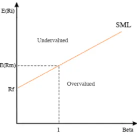
The Security Market Line (SML), or the “Characteristic Line” is a graphical representation of the Capital Asset Pricing Model. SML shows different levels of systematic risk, beta, of different funds at a particular time period which are plotted against the expected return of the market.

Figure 2.1 SML

The graph above represents the SML, where the beta coefficient is the independent variable and the expected return on the asset is the dependent variable. If the fund lies above the line, then it can be said that the fund is undervalued since it performs better than the market, more expected return with equal risk. If the fund lies below the line, then the fund can be

overvalued since it performs worse than the market, lower expected return with equal risk. The SML is often used by investors to evaluate if a fund should be included in a portfolio or not. They usually want to see if the security offers a desirable expected return contrary to the level of risk.

SML is also used often to compare two funds that yield similar returns. It can be seen which fund has the least amount of risk and which fund should be used in the portfolio or funds with similar expected returns can be compared to see which of the funds have higher or lower risk. One should be cautious while using SML, since most of the values except the risk-free rate are historical. Values such as beta and market risk premium have to be calculated while using the SML and these vary frequently over time. This is often considered a disadvantage.

2.3BETA

In finance, beta coefficient 𝛽 indicates whether the investment is more or less volatile than the whole market. It is used to measure the volatility and systematic risk of a portfolio.

Sometimes beta signifies how the returns of an asset respond to sudden changes and swings in the market5.

The value of the beta can be calculated with regression analysis or by dividing the covariance of the returns on the asset and the returns on the market by the variance of the market return. The formula is as follows,

𝛽 =

Covariance is used to see how two different stocks move together. It can be used to measure the relationship between two assets with high risk. The standard deviation, also known as sigma, measures how far each observation is from the mean and sigma squared is equal to the variance. It can be used to calculate the volatility of the stock over a period of time.

Beta has many disadvantages, one of them being that it changes over time. Changes in security beta differ from security to security and some go up and some go down6. The

accuracy of historical betas is hard to estimate, but we could say that these changes most often cancel out in a portfolio and we notice less change in the actual beta on the portfolios than on the funds7. Beta does not include new information, the historical beta cannot capture new substantial risks a company will take on it. It is also said that the pricing movements in the past are not very reliable to predict future values of beta. It is also been suggested by financial advisors that markets do not always provide reliable information and should not be

completely relied on8.

Since risk is affected by numerous factors, it is widely debated among researchers whether beta is an adequate measure for the level of risk. In the late 1970s, researchers have uncovered other variables affecting the average returns provided by beta, such as size, various price ratios and momentum. Fama and French (1998) have done significant research on the validity

5

http://www.diva-portal.org/smash/get/diva2:656578/FULLTEXT01.pdf 6 _{Modern Portfolio Theory and Investment Analysis. (9}th _Edition)

7_{https://www.theseus.fi/bitstream/handle/10024/114240/Postnikova_Ekaterina.pdf?sequence=1}

8_{Accounting based risk measurement: An alternative to CAPM derived discount factors. York: University of} York: The York Management School.

of the CAPM and found that the high average returns observed on stocks with high book-to-market or high earnings-price ratios cannot be explained by the betas for global stock book-to-market portfolio. They argue that the estimate of the beta premium is surrounded by statistical uncertainty and other variables capture variation in expected return. This created a major problem for the CAPM, since portfolios produced a wide range of average returns that are not positively related to market betas (Fama and French, 1998).9

2.4JENSEN’S ALPHA

Jensen’s Alpha, also known as Jensen’s Measure is a performance measure based on CAPM which measures the risk-adjusted performance in relation to expected market return. It was first introduced by Michael Jensen in 1968, and was intended to help evaluate managers in predicting if it is possible to out-do the market but Jensen disagreed10.

Jensen’s alpha is measured by the following equation derived from CAPM, 𝛼_& = 𝑟_&− 𝑟₉+ 𝛽_& 𝑟₊− 𝑟₉

Where, 𝑟_& is the expected return of the portfolio or investment, 𝑟₊ is the expected return of the appropriate market index, 𝑟9 is the risk-free rate of return for the time period and 𝛽& is the

beta of the portfolio of investment with respect to the chosen market index.

If the value of the Alpha is higher, then the portfolio has earned more than it was predicted. It is important since investors need to look at the total return and the total risk of the portfolio that is needed to gain the returns wanted. This measure is also very close to CAPM, because it divides the portfolio in two different parts namely,

1) Focusing on the managers’ ability to forecast future returns and prices with a certain amount of risk.

2) The second part uses efficient diversification to minimize risk.

9_{The Capital Asset Pricing Model: Theory and Evidence, Eugene F. Fama and Kenneth R. French, Journal of} Economics Perspectives, 2004

10

There are some drawbacks on the Jensen’s alpha performance. It is said that managers who earn excess returns are usually derived from luck instead of skill, as referred to in EMH (Efficiency Market Hypothesis) that was founded by Eugene Fama.

2.5TREYNOR MEASURE

The Treynor Measure or Treynor ratio is a reward to volatility ratio. This ratio was named after Jack L. Treynor and is used to measure returns that have been exceeded by those that have made profits on an investment no risk in comparison per unit of market risk. It is similar to the Sharpe Ratio since it is also a return to variability type of ratio. The difference is that Treynor Ratio uses the Beta instead of standard deviation to measure market risk.

Portfolios with a higher return with a risk-free systematic rate have higher Treynor ratio. Short term performances are compared usually by ratios that include Beta in the ratios, especially Treynor. If there is a high value, it signifies that the investment has generated high returns on market risks taken. But it is said that the lower the systematic risk, the better the performance of the ratio11.

The ratio can be expressed in the following way,

𝑇𝑅𝐸𝑌𝑁𝑂𝑅_& = 𝑟&− 𝑟9 𝛽_&

Where 𝑟_& is the average return from portfolio 𝑝, 𝑟₉ is the risk-free rate of interest and 𝛽_& is the beta of the portfolio.

There are some weaknesses with the ratio since it is somewhat backwards. For example, stocks usually perform differently in the future than the past- If a stock will have a Beta of two or three that does not mean that the volatility will be twice or thrice of the market for a long time.

11

2.6 SHARPE RATIO

Sharpe ratio was derived by William Sharpe in 1966 and since then, it has been referred to and used in finance as one of the most referenced risk-return measures. The Sharpe ratio determines the excess return of the portfolio in comparison with the risk-free rate per unit of volatility. If the ratio of the fund is higher, then the returns are said to be better in relation to the amount of investment risk taken. Lower standard deviation and high returns yields high Sharpe ratios. But there could be a controversy about this, because in some cases, having funds with a lower standard deviation can yield a higher Sharpe ratio if they have consistent decent returns12.

The Sharpe ratio focuses on maximizing returns and minimizing volatility. It can be used to calculate the total expected returns in contrast to the risk that investors can take. It is a risk adjusted measure and hence, the relative performance of a portfolio can be permitted since the risk is already taken into consideration.

The ratio is calculated by the following equation:

𝑆𝐻𝐴𝑅𝑃𝐸_& = 𝑟&− 𝑟9 𝜎_&

Where 𝑟_& is the average return from portfolio 𝑝, 𝑟₉ is the risk-free rate of interest and 𝜎_& is the standard deviation of returns for portfolio 𝑝. The nominator 𝑟&− 𝑟9 is also referred as the risk

premium for the portfolio 𝑝.

3.

M

ETHODOLOGY

In this paper empirical analysis will be used to approach our aim. Firstly, time-series

regression to investigate if CAPM holds on the Swedish pension fund market, that is, if alpha is equal to zero. This will be followed by applying the performance measurements, namely the Sharpe ratio, Treynor ratio and Jensen’s alpha to rank the selected funds and analyse the results. Lastly we will use CAPM to predict four of the fund’s annual return and compare it with the actual return. We will use historical from 2009-2016 to make the prediction for 2017. In this section, the method of data selection will be introduced followed by a brief summary of key information on each selected pension funds. We present all the different variables included in the regression, the performance of the regression, how to understand the Durbin Watson and how we will interpret the value of alpha. The quantitative analysis and the

regression is done in Excel on the imported daily closing net asset value for the time period of 2009 to 2017.

3.1 DATA SELECTION

To perform the time series regression on CAPM we set the period from January 2009 to December 2017. The selection of the time period is to avoid abnormal values of beta that might have been caused by the financial crisis 2007-2008. We have collected daily data for all the selected funds.

3.2 SAMPLE SELECTION

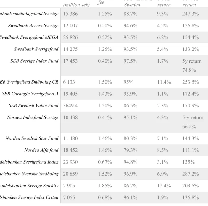
Pension funds based in Sweden has been our goal to find. We initially wanted to find 10-15 funds from each bank but we realized after some research that it was not possible to find that many Swedish based pension funds. We ended up selecting 3-4 funds from each of the four largest banks, Handelsbanken, Swedbank, Nordea and SEB. Mutual funds, pension funds, exist in different shapes, for example index funds, which focus on investing in companies that are part of a major stock indices. We also have stock funds, bond funds and money market funds. Index funds and stock funds are the most common in our selection. We will introduce the funds by displaying a table of key variables. The information was collected Morningstar.13

13

Table 3.1 The selected funds key information

3.3VARIABLES

The daily returns of the funds and the index are calculated by the following formula:

ReturnK=

P_M PMNO− 1

where P_M stands for the value of a fund at time t. P_MNO stands for the value at time t − 1.

Choosing the risk-free rate and the return of the market can be problematic. Since the historical data collected on the funds is based on the Swedish market, it is reasonable to use the Swedish index OMX Stockholm 30 (OMX30), which includes all the four banks

Pension fund Fund value (million sek)

Yearly

fee % invested in _Sweden 1-year _return 10- year _return Swedbank småbolagsfond Sverige 15 386 1.25% 88.7% 9.3% 247.3%

Swedbank Access Sverige 12 007 0.20% 94.6% 4.2% 126.8% Swedbank Sverigefond MEGA 25 826 0.52% 93.5% 6.2% 154.4% Swedbank Sverigefond 14 275 1.25% 93.5% 5.4% 133.2% SEB Sverige Index Fund 17 453 0.40% 97.5% 1.7% 5y return

74.8% SEB Sverigefond Småbolag CR 6 133 1.50% 95% 11.4% 253.5%

SEB Carnegie Sverigefond A 19 405 1.43% 95.9% 1.1% 172.4% SEB Swedish Value Fund 3649.4 1.50% 86.5% 2.3% 170.9% Nordea Indexfond Sverige 10 438 0.41% 95.1% 4.3% 5-y return

66.2% Nordea Swedish Star Fund 11 480 1.46% 80.3% 7.1% 144.3%

Nordea Alfa fond 18 452 1.46% 79.3% 8.5% 111.1% Handelsbanken Sverigefond Index 23 930 0.67% 94.8% 3.1% 135% Handelsbanken Svenska Småbolag 20 859 1.52% 96.9% 6.9% 287.2%

Handelsbanken Sverige Selektiv 2 905 1.85% 86.7% 12.4% 203.5% Handelsbanken Sverige Index Critea 7 055 0.68% 96.1% 1.9% 136.8%

investigated as its components. OMX30 contains of the 30 most traded shares on Nasdaq Stockholm. We collected the data from Vafinans.se.14

The risk-free rate was calculated by taking the daily closing rates of 1-month treasury bill for the time period investigated and taking the average per month of all the daily closing prices. Meaning that the risk-free rate was changed to a new average for every month during the regression. The data was extracted from Riksbank.se.15

3.4 TIME SERIES REGRESSION

Time series analysis is frequently used in world of science to forecast models, estimate dynamic casual effects and measure the price of a stock on the stock market for instance. Time series also comes with some technical issues as time lags and autocorrelation. To perform time series regression, we need to have a data set of 𝑇 observations of a random variable. The observations need to be evenly distributed over time, monthly, daily etc. We will introduce some new variables that we use in the regression:

The excess return of an asset at time 𝑡 is 𝑅_P,QR = 𝑅P,Q− 𝑅9,Q, the return of an asset at time 𝑡

minus the return of the risk-free rate at time 𝑡. The excess return of the market at time 𝑡 is 𝑅_S,QR _{= 𝑅}

S,Q− 𝑅9,Q, the return of the market at

time 𝑡 minus the return of the risk-free rate at time 𝑡.

We have collected historical data for the excess return of the asset 𝑅_P,QR and the excess return of the market 𝑅_S,QR _{over our time horizon. To perform the time series regression, we assume}

the following:

1. We assume that expected returns on the asset, 𝐸[𝑅_P], is constant over the time-period. The actual returns may not be constant but we assume that the expectations are.

14_{https://www.vafinans.se/index/historik/omx/2.1.2009_29.12.2017}

2. We construct a linear regression model: 𝑅_P,QR _{= 𝛼 + 𝛽𝑅}

S,QR + 𝑢Q, where u is some error

term. We assume IDD (independent and identically distributed) across t, that 𝐸 𝑢 = 0 and that 𝐸 𝑢 and 𝑅_SR _{is uncorrelated.}

This regression is performed on all the assets to estimate alpha, beta and u for each fund. If we take expectation of both sides of the regression equation, we obtain the CAPM equation, if alpha is equal to zero.

3.4.1 DURBIN WATSON

The Durbin Watson is a statistical test that measures the autocorrelation in the residuals of a statistical regression analysis. The test looks for a specific type of serial correlation only. It is slightly complex but it includes residuals from a least squares regression on a set of data.

1) The fundamental assumptions in regression is that the error terms have a mean value of zero and constant variance.

2) Regression involves a regressor and response variables that have a natural sequential order with time. This is known as time series data.

3) This test has a base assumption that any error in the regression model is generated by an autoregressive process that is a first order process. It is seen at equally spaced time periods.

The test reports a statistic with common values from 0 to 4, - If the value is at 2, then there is no autocorrelation. - Between 0 and 2 is positive autocorrelation. - Between 2 and 4 is negative correlation.

A main rule is that if there are values between 1.5 and 2.5 in the test, then results are relatively normal.

Hypothesis,

𝐻_X: No first order correlation.

Assumptions,

- The errors normally have a mean distribution of zero - The errors are stationary.

The test uses this formula, where 𝑒_Q are residuals from OLS regression.

𝐷𝑊 =

𝑒

− 𝑒

𝑒

3.5 HYPOTHESIS TEST ON ALPHA

The prediction of the CAPM is that alpha equals zero, which means that the intercept of the regression line is zero. To investigate that, null hypothesis test is applied to see whether Jensen’s alpha is insignificant, i.e. alpha is zero, with the alternative hypothesis of a significant alpha. The null hypothesis is as follows:

𝐻X: 𝛼 = 0

𝐻_O: 𝛼 ≠ 0

In case we fail to reject the null hypothesis the model holds and indicates that high return is caused by systematic risk. If the null hypothesis is rejected, meaning that alpha is significantly different from zero, then CAPM does not hold and the investment has generated a lower or higher return than it was compensated for the volatility risk.

There are two approaches to test null hypothesis: the critical value approach and the P-value approach. The critical value is using test statistic (also known as t-statistic) which is compared to the critical value set by the confidence level and the degrees of freedom of the sample. In this case, the confidence level is set to the most commonly used level of 0.05%. Using a t-distribution table16 for the largest degrees of freedom, we get the critical value of 1.960. This value will be compared to the t-statistic of the alpha for each fund to see if we can reject the null hypothesis or not. The null hypothesis 𝐻X is rejected in favour of the alternative

16

hypothesis 𝐻_{_} if the t-statistic is less than -1.960 or greater than 1.960, which means that alpha is significantly different from zero. Alternatively, using the P-value approach with confidence level 0.05%, we reject the null hypothesis if the P-value of alpha is less than 0.05 in favour of the alternative hypothesis.

3.6 PREDICTION WITH CAPM

CAPM is a recognised tool for investors to predict returns of securities. There exist some limitations concerning this, for example, choosing the risk-free rate, market return and the fact that beta is unstable thorough time.17 We will use our historical data from 2009-2016 to predict the annual return of 2017. We have selected four funds, one each from the four banks. The selection was made based on the betas, leading us to choose two funds with the highest and lowest beta and then two more with values in-between.

To make the prediction we run a new time series regression over our new time period to extract a new beta. Continuing we calculated the arithmetic mean of the return of the market using the formula:

𝐴𝑟𝑖𝑡ℎ𝑚𝑒𝑡𝑖𝑐 𝑚𝑒𝑎𝑛 =𝑋O+ 𝑋g+ ⋯ + 𝑋i 𝑁

In our case when we have daily returns, we added all our daily returns up (𝑋_O+. . +𝑋_i), where s is the total number of observation for the daily return, and divide with the number of years (N) to attain the annual average arithmetic mean.

The risk-free rate is collected from the Swedish Riksbank, selecting the yearly average of one month treasury bills from 2016.18 The motivation for this is that we believe that the risk-free rate from 2016 should not differ much for the next year (2017).

Now we have all the variables we need to perform the prediction through the CAPM equation given below: 𝑅_P = 𝑅₍+ 𝛽(𝑅₊− 𝑅₍) 17 https://hbr.org/1982/01/does-the-capital-asset-pricing-model-work 18 riksbanken.se

To investigate how good this prediction is and how well the funds are preforming we will compare it to the actual annual return of 2017. To attain the annual return, we sum up the daily returns of 2017. We will use the same market return and risk-free rate for all the funds namely, 12% and -0.64%.

4.

R

ESULTS

&

A

NALYSIS

In this section, we will first present and analyse the result from the regression to see if CAPM holds on the Swedish pension fund market. This will be followed by the ranking of the funds using the performance measurements. Lastly, we demonstrate results of the prediction of the future return in 2017 to see whether CAPM is applicable for predictions and if the funds have over-performed or under-performed based on previous years.

4.1 HYPOTHESIS TEST ON ALPHA

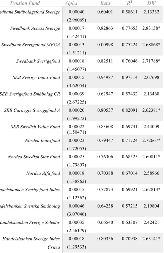
Using the time series regression on the selected funds, we attained certain values for alpha that is the hypothetic intercept of the regression line. To determine whether these values are statistically significant or not, we did null hypothesis test using the t-statistic and the P-value. These values are represented in the table below together with the 𝑅g _{and Durbin Watson}

statistic. The Durbin Watson statistic will be discussed further on to see whether there is any autocorrelation in the residuals of a statistical regression analysis.

Pension Fund Alpha Beta 𝑅𝟐 _DW

Swedbank Småbolagsfond Sverige 0.00040 (2.96069)

0.60401 0.58611 2.13332

Swedbank Access Sverige 0.00017 (1.42441)

0.82863 0.77653 2.83138*

Swedbank Sverigefond MEGA 0.00013 (1.51211)

0.00998 0.75224 2.68868*

Swedbank Sverigefond 0.00018 (1.45077)

0.82511 0.76046 2.71788*

SEB Sverige Index Fund 0.00015 (3.62054)

0.94987 0.97314 2.07698

SEB Sverigefond Småbolag CR 0.00039 (2.67225)

0.62947 0.57432 2.13468

SEB Carnegie Sverigefond A 0.00020 (1.99272)

0.80537 0.82091 2.62381*

SEB Swedish Value Fund 0.00022

(1.50471) 0.83608 0.69731 2.44009 Nordea Indexfond 0.00023

(1.72053)

0.79447 0.71724 2.72667*

Nordea Swedish Star Fund 0.00025 (1.79897)

0.76306 0.68525 2.60811*

Nordea Alfa fond 0.00018 (1.38862)

0.70388 0.67014 2.58966

Handelsbanken Sverigefond Index 0.00015 (1.12362)

0.77873 0.69921 2.62813*

Handelsbanken Svenska Småbolag 0.00046 (3.07046)

0.64238 0.57215 2.19804

Handelsbanken Sverige Selektiv 0.00035 (2.56179)

0.66540 0.63307 2.42421

Handelsbanken Sverige Index Critea

0.00018 (1.29533)

0.80356 0.70938 2.63141*

The t-statistics for the alpha values are represented in parentheses in the table above. We conclude using the null hypothesis test that the following funds do not reject the null hypothesis, meaning that alpha is statistically insignificant (i.e. is zero):

§ Swedbank Access Sverige § Swedbank Sverigefond MEGA § Swedbank Sverigefond

§ SEB Swedish Value Fund § Nordea Indexfond

§ Nordea Swedish Star Fund § Nordea Alfa fond

§ Handelsbanken Sverigefond Index § Handelsbanken Sverige Index Critea

The rest of the funds have rejected the null hypothesis with their t-statistic being greater than the critical value of 1.96. This means that the value of alpha is not zero for those funds. Since the assumption of CAPM is that alpha is zero, we can conclude that CAPM holds for 9 of the 15 funds that have been evaluated. Since alpha is a measure of the excess returns from the asset, funds with alpha value being equal to zero are correctly priced and did not yield returns above or below the risk premium. The funds that rejected the null hypothesis have alpha value greater than 0, which means that they have positive excess return for its level of

undiversifiable risk and were under-priced.

The funds that contain slightly high values of Durbin Watson are marked with a *. Eight out of the fifteen funds indicate slight negative autocorrelation, meaning that a positive error for one observation is often followed by a negative error and vice versa. Field (2009)19 states that values under one and more than three are definite cause for concern and a thumb role is that values between 1.5-2.5 a relatively normal.

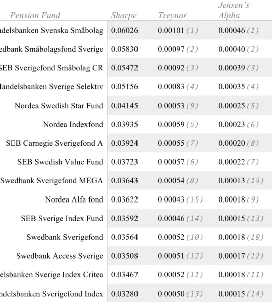
4.2 PERFORMANCE MEASUREMENTS

The table 4.2 represent the ranking of the performance of the funds according to each measurement. All of the funds examined have a reasonable and expected beta, they are

positive which means that the relationship between the risk and return is positively linear. The

19

value of beta also represents the responsiveness of the asset to any change in the index. The three performance measurements - namely the Sharpe ratio, Treynor measure and Jensen’s alpha – have shown a reasonable result: the four top ranked funds are in the same place according to the performance measurement. The rest of the funds are also ranked at a relatively similar place.

Pension Fund Sharpe Treynor Jensen’s Alpha Handelsbanken Svenska Småbolag 0.06026 0.00101(1) 0.00046(1)

Swedbank Småbolagsfond Sverige 0.05830 0.00097(2) 0.00040(2)

SEB Sverigefond Småbolag CR 0.05472 0.00092(3) 0.00039(3)

Handelsbanken Sverige Selektiv 0.05156 0.00083(4) 0.00035(4)

Nordea Swedish Star Fund 0.04145 0.00053(9) 0.00025(5)

Nordea Indexfond 0.03935 0.00059(5) 0.00023(6)

SEB Carnegie Sverigefond A 0.03924 0.00055(7) 0.00020(8)

SEB Swedish Value Fund 0.03723 0.00057(6) 0.00022(7)

Swedbank Sverigefond MEGA 0.03643 0.00054(8) 0.00013(15)

Nordea Alfa fond 0.03622 0.00043(15) 0.00018(9)

SEB Sverige Index Fund 0.03592 0.00046(14) 0.00015(13)

Swedbank Sverigefond 0.03564 0.00052(10) 0.00018(10)

Swedbank Access Sverige 0.03508 0.00051(12) 0.00017(12)

Handelsbanken Sverige Index Critea 0.03467 0.00052(11) 0.00018(11)

Handelsbanken Sverigefond Index 0.03280 0.00050(13) 0.00015(14)

Table 4.2 Ranking of the funds

This result is not surprising since, these investment performance measures tend to rank funds similarly, despite the fact that Sharpe ratio takes into account the standard deviation of the return on the asset whereas Treynor ratio is measured using the beta coefficient.

To decide which measure is more adequate for ranking the performance of the funds, there are several factors to consider. Firstly, Treynor measure is rather sensitive to the market index used to estimate the beta coefficient, but on the contrary it is preferable due to its systematic risk measures which is sometimes more important than total risk in particular cases.

Systematic risk is very important from the investor’s point of view, therefore it is widely used indicator for the evaluation of the asset. The Sharpe ratio is considered as a less precise measurement when volatilities are too diverse. It uses the historical returns for a given time period without evaluating the risk, therefore it is a less desirable measurement used by

investors. The Jensen’s alpha is positive for every fund, and was determined to be statistically insignificant for 9 of the funds that were mentioned in the previous section. This measure also takes into account the systematic risk and contains the benchmark, unlike the previous two measures. It is considered to be useful for evaluating the performance but is not equally preferred for rankings as the other measurements because does not allow assets with different risk to be compared.20 The results of the performance measurements are represented on the graph below.

20

Figure 4.1 Performance of the funds

4.3 PREDICTION OF THE RETURNS

In the table 4.3 we display the results for the prediction of the fund’s annual return 2017 when applying CAPM. The values for return of the market and the risk-free rate was set to 12% and -0.64%. The two columns to the right represents the beta values first for the regression until 2016, which is used in the prediction, the second for the regression until 2017. We can note that in the table the betas only differ very slightly from the previous year, which was

expected. We can also conclude that the higher the beta, the higher predicted return, which is in line with the CAPM theory. Note that the predictions with the two highest betas has yielded the most accurate prediction compared to the actual annual return of 2017.

Prediction test Prediction Actual 𝜷_{𝟐𝟎𝟏𝟔} 𝜷_{𝟐𝟎𝟏𝟕} SEB Sverige Index Fund 11.38% 9.1% 0,95141 0.94987

Handelsbanken Sverige index criteria 9.53% 7.81% 0,80436 0.80356

Nordea Alfa Fund 8.23% 15.08% 0,70167 0.70388

Swedbank småbolagsfond sverige 7.02% 12.11% 0,60569 0.60401

Table 4.3 The prediction test

For the funds with the lowest betas, the prediction is much lower than the actual return. The difference between the expected and the actual return could be questioned. This can be due to many reasons, for example, more active or better fund managers leading to over performing funds.

We should also be aware that these results should be considered with caution since it has limitations, for example the choices of the risk-free rate and the return of the market. It might be more reasonable to compare Swedbank Småbolagsfond Sverige with an index containing smaller cap companies than the OMX30. There are also some limitations with the regression and some possible negative autocorrelation that can be further investigated as mentioned before.

5.

C

ONCLUSION AND SUMMARY

The Capital Asset Pricing Model is used most often to predict returns of securities by investors. We have applied this model and other measures to analyse fifteen funds from the four biggest banks in the Swedish Pension market. A regression analysis was performed to calculate the values of beta and alpha. With these values, we further calculated the Sharpe and Treynor measures. These measurements were used to analyse the performance of the funds and to see if CAPM holds for majority of the funds. A t-statistic test was run to see if the values of alpha was significant or not. The hypothesis test was rejected by six of the funds since the t-statistic value was greater than the critical value, which we found out to be 1.96. We concluded in this section that the value of alpha for these 6 funds was not zero and hence, CAPM does not hold for these funds. If the value of alpha is statistically insignificant, or zero then the model can be applied to the funds. We can thus say, that the funds that don’t have an insignificant value of alpha are under-priced and the funds with alpha that are equal to zero are correctly priced.

In our research work, we have also decided to rank all the funds based on its performance. The ranking is formulated based on the three measurements that were calculated, mainly Jensen’s alpha, Sharpe and Treynor. The values of beta that we calculated turned out positive and thus we can deduce that there is a positive relationship between risk and return. We have seen that the four top ranked funds are in the same place according to the performance measurement. On average most of the funds follow a similar pattern, with all the three measurements. We have calculated that the Handelsbanken Svenska Småbolag has the best ranking with all the three measurements. The Swedbank Smålbolagsfond Sverige and the SEB Sverigefond Småbolag CR rank number two and three respectively.

In the third part of our research we have performed a prediction test on four of our funds for the year 2017. We calculated new betas with historical data until 2016. We found that there was not a very significant difference in the value of beta from 2016 and the beta in the year 2017. Choosing the risk-free rate as -0.6409% from 2016 and the annual average market return of the time period 2009-2016 was 12%. These values were used in CAPM equation to calculate the expected returns of 2017. Two funds namely, SEB Sverige Index Fund and Handelsbanken Sverige index Criteria have higher values of Beta which means there was higher predicted return. Hence, the accuracy of these predictions was the most accurate in relations to the actual values in 2017.

Choosing a risk-free rate for the prediction test was a limitation because one does not know what the real value is and there are many risk-free rates available. Another limitation faced was the negative autocorrelation or the Durbin Watson value during the calculation of the regression. A big problem faced while doing the research was also picking a market return that matches every fund. These values are most often subjected to error.

We could see that the CAPM has some unrealistic assumptions – using beta as a measure of risk is a very big problem since all the values are historic and it is often difficult to see the empirical effects. The model falls short of the expected behaviour of the market, and hence cannot be completely relied on. The theoretical and practical shortcomings of the model cannot prohibit the application of the model since every model in the world of finance has a certain set of limitations. In this research paper we have seen that the model could be applied to predict the performance of the funds and delivered somewhat positive values.

6.

R

EFERENCES

Amenc, N., Le Sourd, V. (2003). Portfolio Theory and Performance Analysis.West Sussex, England: Wiley Finance Series

Fama, E., & French, K. (2004). The Capital Asset Pricing Model: Theory and Evidence.

Journal of Economic Perspectives, 18(3), 25-46.

Field, A. (2009). Discovering Statistics Using SPSS. (3rd ed.). London, England.: Sage Publications.

Francis, J. C., Ibbotson, R. (2002).Investments: A Global Perspective. New Jersey, NJ.

French, Craig W. (2003). The Treynor Capital Asset Pricing Model. Journal of Investment

Management, 1(2), 60-72. Retrieved from: https://ssrn.com/abstract=447580

Goetzman, W. N., Brown, S. J., Gruber, M. J., Elton, E. J. (2014). Modern Portfolio

Theory and Investment Analysis (9th _ed.).

Khalil, M. (2013). Exploring Beta's Changing Behaviour of Swedish Real Estate Stocks. (Master's Thesis, Kungliga Tekniska Högskolan, Stockholm). Retrieved from

http://www.diva-portal.org/smash/get/diva2:656578/FULLTEXT01.pdf

Le Sourd, V. (2007). Performance Measurement for Traditional Investment. Nice, France.: EDHEC Risk and Asset Managment Research Center; Literature Surveys. Morningstar. (2018). Alla Fonder. Retrieved from:

https://www.morningstar.se/Funds/Quickrank.aspx?cb=on

Mullins, D. W. (1982). Does The Capital Asset Pricing Model Work?, Harvard Business

Review. Retrived from: https://hbr.org/1982/01/does-the-capital-asset-pricing-model-work

Pensionsmyndigheten. (2018). Välja fonder i premiepensionen. Retrieved 10.05.2018 from https://www.pensionsmyndigheten.se/forsta-din-pension/valj-och-byt-fonder/valja-fonder-i-premiepensionen

Perold, A. F. (2004). The Capital Asset Pricing Model. Journal of Economic Perspectives, 18(3), 3-24. Retrieved from:

http://www1.american.edu/academic.depts/ksb/finance_realestate/mrobe/Library/capm_P erold_JEP04.pdf

Postnikova, E. (2016). Theoretical and Empirical Analysis of Accounting and Market Betas of Finnish and UK companies. (Bachelor's thesis, JAMK University of Applied Sciences, Jyväskylä). Retrieved from:

https://www.theseus.fi/bitstream/handle/10024/114240/Postnikova_Ekaterina.pdf?sequen ce=1

Sharpe, W. F. (1966). Mutual Fund Performance.The Journal of Business.39(1). 119-138. Retrieved from: http://www.jstor.org/stable/2351741

Statistics How To. (2018). T-Distribution Table. Retrieved from:

Sveriges Riksbank. (2018). Sök räntor & valutakurser. Retrieved from:

https://www.riksbank.se/sv/statistik/sok-rantor--valutakurser/

Toms, S. (2012). Accounting- based Risk Measurement: An Alternative to Capital Asset Pricing Model Derived Discount Factors. Australian Accounting Review, 22(4), 398-406 Va Finans. (2018). Index. Retrieved from:

A

PPENDIX

Selection of funds

We present the funds with some more information.

• Handelsbanken Sverigefond index

Handelsbanken Sverigefond Index is invested 95% in Sweden. The two largest branches are industry and financial service. They strive to mimic the index SIXRX, this index includes 250-300 companies on Stockholm’s stock exchange. Fund assets of 22 949,77 million SEK.

• Handelsbanken Svenska Småbolag

Placement is in smaller and midsized companies in Sweden. Main areas are industry, real estate and consumer cyclical. Fund assets of 19 931,77 million SEK.

• Handelsbanken Sverige Selektiv

Concentrates on a smaller amount of stocks. Long term placements in 16-25 Swedish

companies that has stable profits and strong balance sheets. Industry, technique and consumer cyclical are the largest braches. 86% invested in Sweden. Fund assets of 2 594,65 million SEK

• Handelsbanken Sverige index Criteria

Follows the index SIX SRI Sweden index GI, contains companies reviewed based on ethical criteria’s such as environment, human rights and business ethics. The Fund is invested 96% in Sweden and the main areas are industry and financial service. Fund assets of 6 889,89 million SEK

• Swedbank Robur Småbolagsfond Sverige

Mainly placed in smaller and midsized companies in Sweden. Main areas are industry, consumer cyclical and technique. The fund has assets of 15 386,92 million SEK and are 89% invested in Sweden.

Invests mainly in mid to large cap Swedish companies. Long term horizon with industry, financial service and consumer cyclical as their biggest investment areas. Fund assets of 25 826,12 million SEK.

• Swedbank Robur Sverigefond

Fund assets of 14 275,14 million SEK. Invests in mid and large sized companies, focuses on company selection rather than branches.

• Swedbank Robur Access Sverige

The three biggest branches investments are placed in are industry, financial service and technique. Strive to alike the index OMX Stockholm Benchmark CAP GI, which is an index formed by the largest and most traded stocks on Nasdaq OMX Stockholm AB. Fund assets of 12 007,66 million SEK

• Swedbank Penningsmarknadsfond

Fund assets of 18 067,86 million SEK. This is a money market fund, invests in securities with short maturity and high credibility. Uses mainly money market instruments and obligations issued by the Swedish State.

• Nordea Indexfond

Fund assets of 10 437,93million SEK. Follows the index OMX Stockholm Benchmark cap 100%. It’s 95% invested in Sweden and the main areas are industry, financial service and technique.

• Nordea Alfa Fond

Mainly place investments in Sweden (79%), the rest is placed in the Nordic stock market. Does a thorough analysis of companies to find undervalued stocks. Placements are long term and the fund consists of approximately 30 different stocks. The largest areas are financial service, industry and consumer cyclical.

• Nordea Swedish Star fund

Like the fund Nordea Alfa, Nordea Swedish star fund has the same set up, the difference is the selection. The choosing of the companies is made by a combination of financial analysis

and analysis on how the companies manages risk and opportunities regarding the

environment, social questions and business moral. Fund assets of 11 479,75 million SEK.

• SEB Sverige Index Fund

Does placements in stocks and stock related instruments that are traded on Swedish stock market. The goal is to follow the index SIX Return Index. The management team strive to trade cost efficient and at the same time avoid risk. The main branches of investment are in financial service, industry and consumer cyclical. Fund assets of 17 453,64 million SEK.

• SEB Sverigefond Småbolag CR

Fund assets of 6 133,46 million SEK. This stock fund mainly place in Swedish small cap companies. In the process of selecting companies the management team put effort in the fundamental analysis and meeting the companies they invest in. The largest areas are industry, technique and real estate.

• Carnegie Sverigefond A

Carnegie Sverigefond is an actively managed stock fund that invests long term on the

Swedish stock exchange. They look for stable companies with strong balance sheets etc. The fund is 100% invested in Sweden and two biggest branches are industry and financial service. Fund assets of 18 818,81 million SEK.

• SEB Swedish Value Fund

Mainly invests in mid to large cap companies. The placements are 87% in Sweden and the main areas are industry and financial service. Fund assets of 3 649,4 million SEK.

T-statistic analysis

Swedbank Småbolagsfond Sverige – Reject (2.96>1.96) – Alpha is NOT zero

Swedbank Access Sverige – Do not reject – Alpha is zero

Swedbank Sverigefond MEGA – Do not reject – Alpha is zero

Swedbank Sverigefond – Do not reject – Alpha is zero

SEB Sverige Index Fund – Reject – Alpha is NOT zero

SEB Carnegie Sverigefond A – Reject – Alpha is NOT zero

SEB Swedish Value Fund – Do not reject – Alpha is zero

Nordea Indexfond – Do not reject – Alpha is zero

Nordea Swedish Star Fund – Do not reject – Alpha is zero

Nordea Alfa fond – Do not reject –Alpha is zero

Handelsbanken Sverigefond Index – Do not reject – Alpha is zero

Handelsbanken Svenska Småbolag – Reject – Alpha is NOT zero

Handelsbanken Sverige Selektiv – Reject – Alpha is NOT zero

Graphs

The graphs below represent the regression line for each fund that has been analysed in this paper. The graphs show the linear relationship between the excess return on the market (horizontal axis) and the excess return on the fund (vertical axis). The equation of the regression line is shown in each figure, including the value of beta (slope) and the alpha (intercept). y = 0,7787x + 0,0002 R² = 0,69921 -0,08 -0,06 -0,04 -0,02 0 0,02 0,04 0,06 0,08 0,1 -0,1 -0,05 0 0,05 0,1

Handelsbanken Sverigefond Index

y = 0,6424x + 0,0005 R² = 0,57215 -0,08 -0,06 -0,04 -0,02 0 0,02 0,04 0,06 0,08 -0,1 -0,05 0 0,05 0,1

y = 0,6654x + 0,0003 R² = 0,63308 -0,08 -0,06 -0,04 -0,02 0 0,02 0,04 0,06 0,08 -0,1 -0,05 0 0,05 0,1

Handelsbanken Sverige Selektiv

y = 0,8035x + 0,0002 R² = 0,70938 -0,08 -0,06 -0,04 -0,02 0 0,02 0,04 0,06 0,08 0,1 -0,1 -0,05 0 0,05 0,1

Handelsbanken Sverige index

y = 0,604x + 0,0004 R² = 0,58611 -0,08 -0,06 -0,04 -0,02 0 0,02 0,04 0,06 -0,1 -0,05 0 0,05 0,1

Swedbank Småbolagsfond

y = 0,8248x + 0,0002 R² = 0,75224 -0,08 -0,06 -0,04 -0,02 0 0,02 0,04 0,06 0,08 -0,1 -0,05 0 0,05 0,1

Swedbank Sverigefond MEGA

y = 0,8251x + 0,0002 R² = 0,76046 -0,08 -0,06 -0,04 -0,02 0 0,02 0,04 0,06 0,08 -0,1 -0,05 0 0,05 0,1

Swedbank Sverige Fond

y = 0,8286x + 0,0002 R² = 0,77653 -0,08 -0,06 -0,04 -0,02 0 0,02 0,04 0,06 0,08 -0,1 -0,05 0 0,05 0,1

y = 0,7945x + 0,0002 R² = 0,71725 -0,08 -0,06 -0,04 -0,02 0 0,02 0,04 0,06 0,08 0,1 -0,1 -0,05 0 0,05 0,1

Nordea Indexfond

Nordea swedish stars

y = 0,7039x + 0,0002 R² = 0,6701 -0,08 -0,06 -0,04 -0,02 0 0,02 0,04 0,06 0,08 -0,1 -0,08 -0,06 -0,04 -0,02 0 0,02 0,04 0,06 0,08

Nordea Alfa

y = -0,0001x - 1E-04 R² = 2,2E-05 -0,001 -0,0005 0 0,0005 0,001 0,0015 -0,1 -0,08 -0,06 -0,04 -0,02 0 0,02 0,04 0,06 0,08

Nordea Swedish Bond Stars

y = 0,9499x + 0,0002 R² = 0,97314 -0,1 -0,08 -0,06 -0,04 -0,02 0 0,02 0,04 0,06 0,08 -0,1 -0,08 -0,06 -0,04 -0,02 0 0,02 0,04 0,06 0,08

SEB Sverige indexfund

y = 0,6295x + 0,0004 R² = 0,57432 -0,08 -0,06 -0,04 -0,02 0 0,02 0,04 0,06 -0,1 -0,05 0 0,05 0,1

Durbin Watson

The Durbin Watson is a statistical test that measures the autocorrelation in the residuals of a statistical regression analysis. The test looks for a specific type of serial correlation only. It is slightly complex but it includes residuals from a least squares regression on a set of data.

4) The fundamental assumptions in regression is that the error terms have a mean value of zero and constant variance.

5) Regression involves a regressor and response variables that have a natural sequential order with time. This is known as time series data.

y = 0,8054x + 0,0002 R² = 0,82091 -0,08 -0,06 -0,04 -0,02 0 0,02 0,04 0,06 0,08 -0,1 -0,05 0 0,05 0,1

Carnegie Sverigefond A SEB

y = 0,8361x + 0,0002 R² = 0,69731 -0,08 -0,06 -0,04 -0,02 0 0,02 0,04 0,06 0,08 -0,1 -0,05 0 0,05 0,1

6) This test has a base assumption that any error in the regression model is generated by an autoregressive process that is a first order process. It is seen at equally spaced time periods.

The test reports a statistic with common values from 0 to 4, - If the value is at 2, then there is no autocorrelation. - Between 0 and 2 is positive autocorrelation. - Between 2 and 4 is negative correlation.

A main rule is that if there are values between 1.5 and 2.5 in the test, then results are relatively normal. If there are other values then there should be some certain. Hypothesis,

𝐻_X: No first order correlation. 𝐻_O: First order correlation exists.

Assumptions,

- The errors normally have a mean distribution of zero - The errors are stationary.

The test uses this formula, where 𝑒_Q are residuals from OLS regression.

𝐷𝑊 =

𝑒

− 𝑒

𝑒