The accuracy of the LSTM model for predicting the S&P 500 index and the difference between prediction and backtesting

(1)

IN

DEGREE PROJECT TECHNOLOGY, FIRST CYCLE, 15 CREDITS

,

STOCKHOLM SWEDEN 2018

The accuracy of the LSTM model

for predicting the S&P 500 index

and the difference between

prediction and backtesting

WAR AHMED

(2)

The accuracy of the LSTM model for predicting the S&P 500

index and the diﬀerence between prediction and backtesting

War Ahmed Mehrdad Bahador

Supervisor: Arvind Kumar Examiner: Örjan Ekeberg

A thesis submitted in fulfillment of the requirements for the degree of Bachelor in Computer Science in the

(3)

Abstract

In this paper the question of the accuracy of the LSTM algorithm for predicting stock prices is being researched. The LSTM algorithm is a form of deep learning algorithm. The algorithm takes in a set of data as inputs and finds a pattern to dissolve an output. Our results point to that using backtesting as the sole method to verify the accuracy of a model can fallible. For the future, researchers should take a fresh approach by using real-time testing. We completed this by letting the algorithm make predictions on future data. For the accuracy of the model we reached the conclusion that having more parameters improves accuracy.

(4)

Referat

Med hur stor noggrannhet kan man med en LSTM-model

förutsäga S&P 500 index och skillnaden mellan förutsägelse och

backtesting

I detta arbete forskas det kring hur bra prognoser man kan ge genom att använda sig av LSTM algoritmen för att förutspå aktiekurser. LSTM-algoritmen är en form av djupinlärnigsmetod, där man ger algoritmen en del typer av data som input och hittar ett mönster i datan vilket ger ett resultat. I vårt resultat kom vi fram till man ej ska förlita sig på backtesting för att verifiera sina resultat utan även använda modellen till att göra prognoser på framtida data. Vi kan även tillägga att tillförlitlighet ökar om man använder sig av flera faktorer i modellen.

(5)

1 Introduction

1.1 Definition of the research space

In the last decades the financial landscape has changed dramatically, in all sub sectors of the financial sector there is today some form of combination with technology. The investing busi-ness, compromised of hedge funds, pension funds, mutual funds and sovereign wealth funds have adapted to the uprising of technology in finance, by investing in it and incorporating it in their investment process. What once seemed to be an investment technique used by the few is now used by the masses, the technique referred to is known as quantitative investing. In the financial markets investors are chasing higher returns, the funds specialized in this field are the quantitative hedge funds. In the Quantitative investing landscape there is a myriad of strategies, the one which is the focus of this report is the Neural Network model, with the type of model being a Recurring Neural Network (RNN). Under the RNN scope there are the LSTM algorithms that have recently been incorporated in various stock predicting algorithms and strategies because of their eﬀectiveness compared to other neural algorithms.

Making predictions in stock prices are in fact solving a time series prediction problem. For any algorithms to be able to have a reasonable eﬀectiveness in predicting time series there must be a pattern in the time series, for example there can be a seasonality pattern in the time series or other forms of anomalies. If the time series data is completely random, there can not be a prediction made.

As mentioned earlier there are a wide variety of Quantitative methods to predict stock prices, the method discussed in this report is simply focused on making time series predictions. In our view the final output of the prediction will be more accurate the more data we can feed the model. By this we mean that instead of inputting only the stock prices, other factors that can move the stock price should be inputted as well.

Finally, LSTM is according to research one of the most suitable algorithms for time series pre-dictions compared to CNN (Convolutional Neural Networks), we hold the same view based on our results and the logic behind the usage of both algorithms, where CNN is favored for other usages.

(8)

1.2 Aim and research questions

Our main focus is to study the effectiveness of the LSTM algorithm for prediction of stock prices. Hence the question is not whether they are effective or not, but how accurate a LSTM model can predict the S&P 500 index adjusted closing price through a backtesting method and see how much the deviation was from the real data. We also have the goal of using the Predict function to make real predictions with the algorithms and not just take backtesting data. The reason for this is that there is a risk for overfitting in the models. A lot of individ-uals building their own models use backtesting to claim that they have very high accuracy, if things were that simple, there would be many wealthy data scientists. Their reports often do not mentioned the backtest overfitting which leads to that they look good on paper but a real time simulation will not even be near the accuracy of the backtest result (Bailey et al., 2016a). Thus our final goal is to measure the real effectiveness of LSTM models, using real-time pre-dictions and backtesting. And find methods to improve the accuracy.

Specifically, the goal of the study is to answer the following questions:

• How accurate can an optimized LSTM model predict S&P 500 index price based on back-testing?

• How eﬀective is the LSTM when comparing backtesting with real-time prediction?

1.3 Scope

In the beginning of this project we reached the conclusion that our scope must be as clear and defined as possible, given the large landscape of options that we can study. The main focus of this report will be on LSTM algorithms. The reason we choose LSTM is because of the algo-rithms abilities to consider long-term dependabilities thus making it a good algorithm for time series predictions.

(9)

2 Background

In the research report we have been covering ground on various diﬀerent scientific topics, the background section is divided into sections consisting of mathematical background and a com-puter science background. The fields of comcom-puter science and mathematics are closely inter-twined. As an example in the field of neural networks the usage of mathematics is paramount to the field, hence the reader needs a certain aptitude of mathematics to cope with the com-puter science concepts.

2.1 Artificial Intelligence

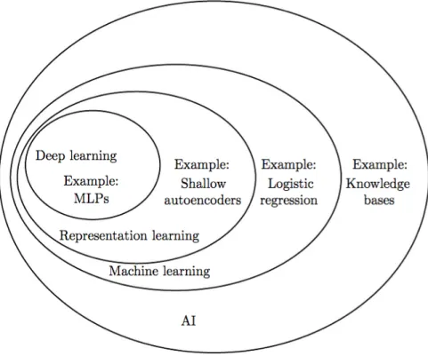
Artificial intelligence also known as AI, is a term used in business, science and nearly any field that it can be applied to. Artificial intelligence has the goal of building and understanding intelligence, this means entities that are intelligent in a way that they can analyze data and recognize patterns. With artificial intelligence predictive analytical methods can be created (Russell and Norvig, 2016).

Figure 1: Venn diagram showing how machine learning, AI, Deep Learning etc. correlate (Singh, 2017)

2.2 Machine learning

Machine learning, also referred to as ML, is a tool for processing and finding patterns in data. Machine learning algorithms focus on optimizing and finding regularities in the data. A big part of machine learning consists of mathematics, the mathematics used is statistical learning and optimization of the data.

A big risk factor in machine learning is the risk of overfitting. Overfitting is when the algo-rithms relay too much on the sample and historical data, placing an all too high weight on the

(10)

historic parameters, and eventually overfitting the data. The problem occurs when the pre-diction is being made of unknown data, the result is a high error rate due to the overfitting. Therefore most scientists and researchers work with hybrid methods on machine learning to minimize this risk as much as possible. Another important aspect related to machine learning that one needs to take into consideration is the representation of data. The data needs to be represented in a structured and accessible manner. The structure is important because it can help the algorithm to process the data correctly (Nasrabadi, 2007).

2.3 Neural networks

Neural networks (NN) is a technological concept capturing the scope of machine learning and the biological brain. The neural networks are built up by a network of neurons or nodes. The lines connecting the nodes are named edges. The nodes in the network receive information as an input from the edges in the network. The information inputted into the nodes is multiplied by the weight set by the constructor of the network. The weight is used to adjust the impor-tance of diﬀerent computational results from the given node. The non-linear function is then added to the result, this function is referred to as the activation function. Typically the acti-vation function is a tan(h) function, and regulates how much of the weighted result from the neurons is added to the output, which can be the final output or an output passed on to more neurons or nodes in the network, in such a case our network will have multiple layers (Schmid-huber, 2015).

2.3.1 Recurrent neural networks

RNN are a class of neural networks that have the ability to have memory, which makes them more similar to how we humans process information and it is an eﬃcient way to solve vari-ous scientific problems. In a traditional neural network the data is processed independently. RNN are better than traditional neural networks in the case of predicting the next word in a sentence thanks to their ability to have a memory and recognize the context (Zaremba et al., 2014).

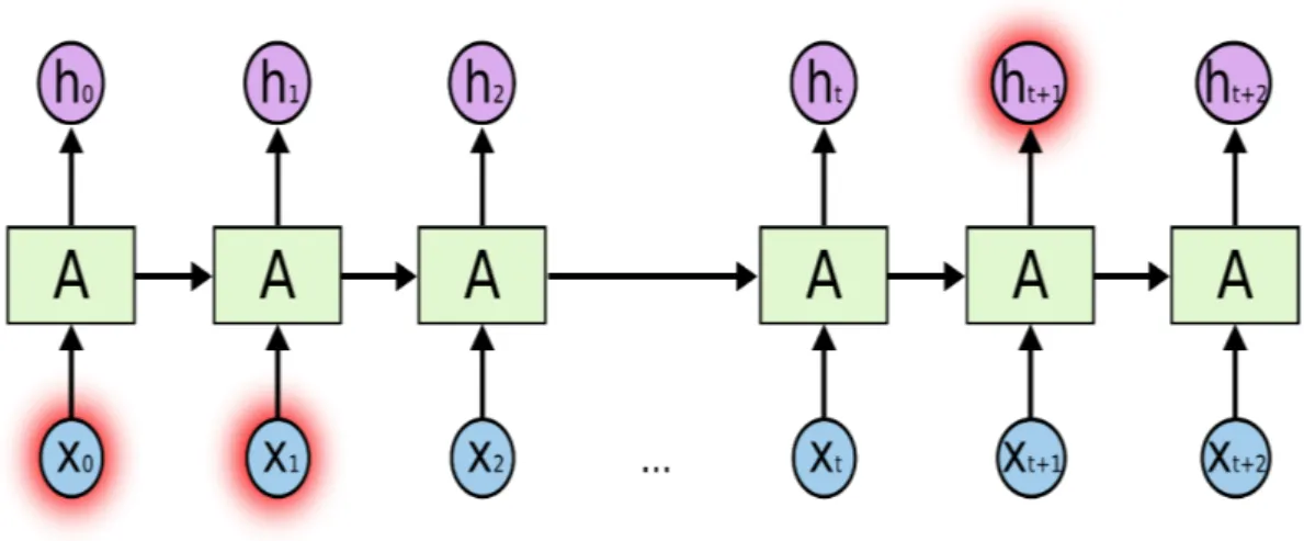
2.3.2 Long-term dependencies

Long-term dependency is a problem that occurs in RNN when the network is in the need of making a prediction that requires context. In a regular RNN the need of understanding the context can be handled but this is dependent on how far back the memory needs to save the information for the context. In a case of predicting a context in a simple sentence where the RNN has to look back a series of words it is doable for the RNN. However, in a situation where the algorithm is required to have memory of a paragraph, it is much more diﬃcult. In theory this can be still achieved in an RNN, if the parameters are adjusted correctly by hand. Fortunately, scientist do not need to put their time info adjusting parameters of a classic RNN and can instead use an LSTM (Gers et al., 1999).

(11)

Figure 2: Long-term dependencies (Olah, 2015) 2.3.3 Long short-term memory (LSTM)

LSTM is a kind of RNN, that has the ability to consider the long term dependability. LSTM was developed by two scientists, Schmidhuber and Hochreiter in 1997. What sets LSTM’s apart from other RNN approaches is that LSTM’s have the ability to remember information for a longer time period and avoid the long term dependabilities. LSTM’s have a chain struc-ture and on the inside they operate using gates and layers of neural networks like other RNN approaches. The structure of the LSTM is constructed in a manner of a cell state that runs through the entire LSTM, the value is changed by the gates that have function by either al-lowing or disalal-lowing data to be added to the cell state. There are also components by the name of gated cells that allow the information from previous LSTM outputs or layer out-puts to be stored in them, this is where the memory aspect of LSTM’s kick in (Hochreiter and Schmidhuber, 1997).

Figure 3: Long short-term memory algorithm (Olah, 2015)

2.4 Data mining

Data mining is the process of extracting valuable data and analytic insights from a large data set. The motives behind this is to predict trends and extract valuable insights from the data (Hand, 2007).

(12)

2.5 Statistics

2.5.1 Regression Analysis

In mathematics the goal of regression analysis is to find correlations and model the relation between one or more dependent or independent variables. The strength of the relationships

vary and it is an important part of the final result to be aware of the relationship and its strength. There are diﬀerent forms of regressions, the most simple form is the linear regression. Linear regression states that there is a linear relationship between the variables, meaning that the relationship can be summarized in a formula: y = ↵ + x.

To represent more complex relations that the linear model does not cover, we can use a simple regression model.

yi= ↵ + xi+ ✏i (1)

where ↵ and represents the parameters, xi the independent variable and ✏i the error term. If the simple linear model does not suits for finding the correlations then the linear regression model can be expanded further by adding additional variables to the model, if we assume that we have a parabola function, we will get the following model.

yi = 0+ 1xi+ 2x2i + ✏i (2)

where 0 2 represents the parameters.

The error is calculated by calculating the diﬀerence between the true value and the predicted value, where Yi is the actual value and ˆYi is the predicted value.

✏i= Yi Yˆi (3)

2.5.2 Mean Squared Error (MSE)

MSE is another method if computing the accuracy and the error in the predictive models used. M SE = 1 n n X n=1 ⇣ Yi Yˆi ⌘2 (4) ˆ

Yi is the ith predicted value and Yi is the ith actual/observed value. 2.5.3 Root-mean-square deviation (RMSE)

RMSE is a method to calculate the error or accuracy in the prediction of ones models. The RMSE calculates the error based on standard deviations. The final output is given in a stan-dard deviation of the magnitude of the error, the individual calculations are outputted as residuals. (Willmott and Matsuura, 2005)

RM SE = v u u tPnn=1 ⇣ Yi Yˆi ⌘2 n (5) ˆ

(13)

Alternatively

RM SE =pM SE (6)

2.5.4 Mean absolute percentage error (MAPE)

MAPE is a mathematical formula that gives us the ability to calculate the accuracy of our forecast. This is an important part of our report given the fact that we rely heavily on fu-ture estimates and are making active predictions of fufu-ture data sets, thus giving ourselves and other constituents the ability to know the accuracy of the prediction is paramount. The cal-culation is done by taking the diﬀerence between the actual value and the forecast value and dividing the diﬀerence by the actual value. In the later stage it is multiplied by the number of data points and 100 to yield the percentage error. (De Myttenaere et al., 2016)

M AP E = 100 n n X n=1 At Ft At (7)

where At is the actual value and Ft is the forecast/predicted value.

2.6 Trading Strategy

A trading strategy can be designed in various ways, there are a large selection of strategies ranging from technical indicator to fundamental indicators. In the fundamental indicators the categories can be divided in bottoms up or tops down. These two terms refer to the way fun-damental parameters are viewed, the bottom up parameters are the basic company metrics such as how much the company is making in earnings and how much debt the company has. The top-down approach is focused on how the economy in general is evolving, as an example that would be if we see the BNP per capita in Sweden increasing we would assume that the people in Sweden have a higher disposable income thus companies selling consumer products are going to increase sales.

In our case our trading strategy is revolving around a technical strategy, this might not pro-duce the most optimal results because historical backtesting has displayed that the hybrid version of a fundamental and technical strategies yield the best results. However, our goal is not to get the best trading results but to research the technology driving it. The reason our strategy is purely technical is because we are looking at indicators such as the volume and the historical price to find buy and sell signals in the patterns (Conrad and Kaul, 1998).

2.6.1 Volume

Trading volume is a measure used in the financial markets on all securities that are traded on an exchange to measure how many contracts or shares have been transacted both on the buying and selling side during a given time period (Conrad and Kaul, 1998).

(14)

3 Method

For measuring the accuracy of LSTM for predicting the S&P 500 Index, a model was imple-mented using the Keras framework and trained using a dataset that contained data about the price of the index. Furthermore this chapter describes how the diﬀerent hyperparameters of the LSTM model were chosen.

3.1 Data Collection

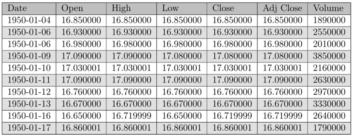
The data of the S&P 500 index price was collected from Yahoo! Finance in the file format comma-separated value (.csv) (Finance, 2018). The dataset contained data about the prices from 1950-01-03 to 2018-03-09, where it was presented in tabular form. Below is a sample of the index price.

Date Open High Low Close Adj Close Volume

1950-01-04 16.850000 16.850000 16.850000 16.850000 16.850000 1890000 1950-01-06 16.930000 16.930000 16.930000 16.930000 16.930000 2550000 1950-01-06 16.980000 16.980000 16.980000 16.980000 16.980000 2010000 1950-01-09 17.090000 17.090000 17.080000 17.080000 17.080000 3850000 1950-01-10 17.030001 17.030001 17.030001 17.030001 17.030001 2160000 1950-01-11 17.090000 17.090000 17.090000 17.090000 17.090000 2630000 1950-01-12 16.760000 16.760000 16.760000 16.760000 16.760000 2970000 1950-01-13 16.670000 16.670000 16.670000 16.670000 16.670000 3330000 1950-01-16 16.650000 16.719999 16.650000 16.719999 16.719999 2640000 1950-01-17 16.860001 16.860001 16.860001 16.860001 16.860001 1790000

Table 1: Dataset from Yahoo! Finance 3.1.1 Description Of Each Data Feature

• Date: The date of that trading day.

• Open: The price of the stock at the very beginning of that trading day but opening price does not need to be equal to the previous day’s closing price.

• High: The highest price the stock had during that trading day. • Low: The lowest price the stock had during that trading day. • Close: The price of the stock at closing time of that trading day.

• Adj Close: The adjusted closing price is the closing price of the stock that has been changed to include any distributions and corporate actions that occurred during that trading day.

• Volume: The number of stocks that were traded during that trading day.

3.2 Data formatting

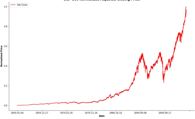
3.2.1 Normalization

Before the dataset that we collected from Yahoo! Finance is used by the LSTM model we en-coded all data in the used categories as numbers. For improving the accuracy of various

(15)

ma-chine learning methods/models, normalization was applied to all data in the features (James et al., 2013).

Figure 4: Normalized Adjusted Closing Price

The data of each feature that is used by the LSTM model is normalized and table below shows that in tabular form.

Date Open High Low Close Adj Close Volume

1950-01-04 0.000070 0.000063 0.000071 0.000071 0.000063 0.000071 1950-01-05 0.000098 0.000091 0.000099 0.000099 0.000091 0.000099 1950-01-06 0.000116 0.000109 0.000116 0.000116 0.000109 0.000116 1950-01-09 0.000154 0.000147 0.000152 0.000152 0.000144 0.000152 1950-01-10 0.000133 0.000126 0.000134 0.000134 0.000126 0.000134 1950-01-11 0.000154 0.000147 0.000155 0.000155 0.000147 0.000155 1950-01-12 0.000039 0.000032 0.000039 0.000039 0.000032 0.000039 1950-01-13 0.000007 0.000000 0.000007 0.000007 0.000000 0.000007 1950-01-16 0.000000 0.000018 0.000000 0.000000 0.000018 0.000000 1950-01-17 0.000074 0.000067 0.000074 0.000074 0.000067 0.000074

Table 2: Normalized Data 3.2.2 Percentage Change

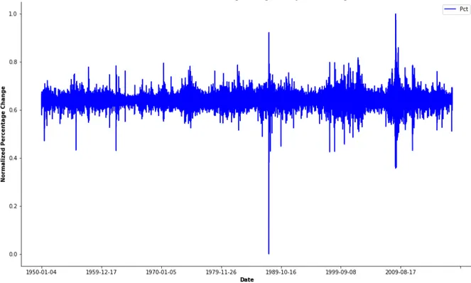
The figure below shows the normalized percentage change of adjusted closing price, this fig-ure indicate how volatile the S&P 500 have been during its time. The more volatile the index is then that corresponds to a more aggressive price change over a explicit time period. Over the time the S&P 500 index have been relative stable with a low volatile price change during

(16)

long periods (Harris, 1989), which we can also see from the Figure 5 that the index have been stable except from the years 1987-1988 and 2007-2009.

Figure 5: Normalized Percentage Of Change Of the Adjusted Closing Price 3.2.3 Necessary Index Features

All the features that are included in the data set are not necessarily fundamental for the LSTM model to have as input for predicting the adjusted closing price with great accuracy. We cal-culated the coeﬃcient of determination for each data features the index has, the table below shows what each feature scored. The coeﬃcient of determination score is between 0 and 1, where 1 indicates that the model of that feature is a perfect fit.

We split the data into sets of training and testing using each given feature as target, we then created a decision tree with the depth set to maximum and fit it to the training set. We then got a coeﬃcient of determination for each feature which is shown in the table below.

Feature R2_Score Open 0.999916 High 0.999957 Low 0.999947 Close 0.999997 Adj Close 0.999997 Volume 0.440008 Table 3: R2_Score

Table 3 conclude the coeﬃcient of determination score, it looks like the features Open, High, Low, Close and Adj Close, where Close and Adj Close has the highest relevancy.

(17)

Vol-umehas the lowest score and will not be included in the prediction because the model of that feature could not fit when predicting them using the other features.

3.2.3.1 Visualization Of Feature Distributions

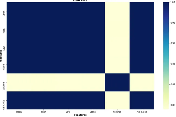
For our visualization and getting a better understanding of the coeﬃcient of determination score that we got we created a heat map over the index features. We can see that it is a cor-relation between features Open, High, Low, Close and Adj Close from 6. If we look at the feature Volume we see that the heat map does not show any correlation, there is no linear correlation between the rest of the features and should therefore be excluded in the prediction.

Figure 6: Heat Map Of The Six Index Features

3.3 Frameworks

The LSTM model was constructed and trained with the Keras neural network API (Keras, 2018a). The API is a open source deep learning library written in Python and uses Tensor-flow as backend. TensorTensor-flow is also an open source machine learning framework for numerical computations (Tensorflow, 2018). Keras fast learning curve and together with its easy imple-mentation of deep learning models made a great tool for us to use for this project.

3.4 LSTM Structure

The LSTM model’s performance depends solely on the hyperparameter settings and the amount of training. The settings of the model are presented below.

(18)

3.4.1 Input

We represent every trading day in our dataset as a vector of the size 1x5, where 5 is equal to the number of features that we would include in our prediction. Together with all of the trading days and their features which are included in the prediction we constructed a ma-trix and split all of the trading days into windows of a fixed size length. Then we reshape the all the vectors in the matrix so that we get a numpy array that is now a 3D vector of the shape (W ⇥ l ⇥ f), where W = Number Of W indows, l = Length Of A W indow and f = N umber Of F eatures. This partitioning of the dataset was done in order to calculate the output easier and to support the input format of our framework Keras.

We then split the dataset into train and test sets where the training set contained 90% of the dataset (trading days) and the rest (10%) were the test set. We then train the LSTM Model to determine the price of the adjusted closing price for each training day because it has the highest relevance according to table 3.

3.4.2 Layer

3.4.2.1 Hidden Layer

When constructing the LSTM model we have to take into consideration how many hidden lay-ers the model will contain, the amount of LSTM cells that should be included in every layer and what the dropout should be. There is no right or wrong way of choosing the number of hidden layers or the number of cells within each layer, we have seen successful models where one model contained 4 layers and 1000 cells (Sutskever et al., 2014) and the other model con-tained 3 layers and 2 cells (Gers et al., 2000). These number depends on what application the LSTM model is going to be used on, so the number of cells and layers can diﬀer but the layers are often from 1 to 5 and the cells in each layer should contain the same amount of cells for finding an optimal structure.

3.4.2.2 Dense Layer

A dense layer is a densely connected NN layer (Keras, 2018b), where a dense layer connects each cell to another in the next layer. We have seen successful models using dense layer by building their model of hidden layers followed by multiple dense layer (Goodfellow et al., 2013). 3.4.2.3 Number Of Layers

We have decided that our LSTM model will contain four layers, two hidden layers and two dense layers. The output of the first hidden layer is connected to another hidden layer than that layer is connected to a dense layer and that dense layer is lastly connected to another dense layer, i.e. hidden layer ! hidden layer ! dense layer ! dense layer, where ! rep-resent the connection between layers. Dropouts are used after each hidden layer for preventing the risk of overfitting (Reimers and Gurevych, 2017).

3.5 Optimal Hyperparameters

While building the LSTM model there are hyperparameters that have to be setup properly and adjusted so that we can get an accurate prediction when backtesting our model. This pa-per by (Reimers and Gurevych, 2017) have inspired us on how we could do empirical tests for finding the optimal hyperparameters that will lead to higher accuracy and minimize the risk of overfitting the data, compared to if no empirical test was done to our model and data.

(19)

When doing the empirical test we will build our LSTM model with default hyperparameters that fit our case best according to diﬀerent papers that we find highly valuable. We will then take each hyperparameter one by one and try to find a optimal value to that hyperparameter. The best value for a hyperparameter is found by evaluating the LSTM model by backtesting it with the test data. We will then calculate the MSE between the model’s prediction on the adjusted closing price and the actual closing price for that day. After all potential values for that specific hyperparameter has been evaluated we will plot on the x-axis the hyperparameter value and on the y-axis the MSE value. We can then see that the hyperparameter value with lowest MSE is the most optimal one.

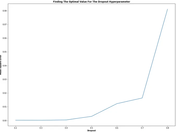
3.5.1 Dropout

The dropout is an important technique that reduces overfitting by randomly choosing cells in a layer according to the probability chosen and set their output to 0 (Srivastava et al., 2014). An empirical test was done to find the optimal amount of dropout and was then applied to all of the hidden layers. We built our LSTM model and trained the model, we then set the dropout to diﬀerent values where the diﬀerence between the consecutive dropout value is con-stant. From fig. 7 the we can see that the optimal dropout value in our case is 0.3 because that value has the smallest MSE, hence the dropout is set to 30%.

While doing this empirical test the epoch was set to 220, the LSTM cells in each layer was set to 128, 128, 64 , 1, decay to 0.2 and the length of window to 22.

(20)

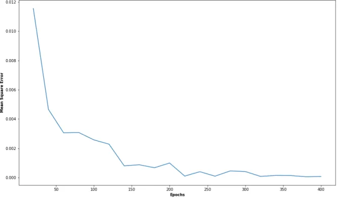
3.5.2 Number Of Epochs

An epoch is when the whole training data has been passed through the network, hence one epoch is one iteration of the whole training data being passed through the network (Kaastra and Boyd, 1996). When the training data are being propagated through the network we split the training data into a batch size, where we defined the batch size as 512. This means that first the 512 samples are being taken from the training data (0-511) and trained on the net-work, then it takes the next 512 samples (512-1023) and trains the network. The epoch con-tinues until all samples are propagated through the network hence then one epoch had been passed through the network (Reimers and Gurevych, 2017).

From fig. 8 we can see that the optimal epoch value in our case is 380 because that value has the smallest MSE. While doing this empirical test the dropout was set to 0.3, the LSTM cells in each layer was set to 128, 128, 64 , 1, decay to 0.2 and the length of window to 22.

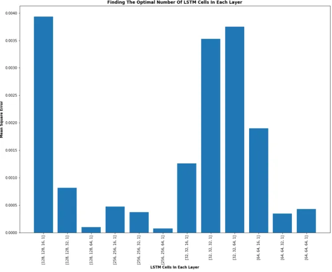
Figure 8: Illustrating empirical testing for finding the optimal epoch value 3.5.3 Number Of LSTM Cells In Each Layer

Every hidden and dense layer has a number of LSTM Cells, we want to find the most optimal number of cells for each layer. We find a successful report that had the same number of cell (250 cells) in each hidden layer (Graves et al., 2013). We trained the network with diﬀerent values on each cells in the hidden and dense layer, from fig. 9 we can see that the cells in each layer in our case should be set to 256, 256, 64, 1 because that value has the smallest MSE. While doing this empirical test the dropout was set to 0.3, epoch to 380, decay to 0.2 and the length of window to 22.

(21)

Figure 9: Illustrating empirical testing for finding the optimal value for the neurons. 3.5.4 Decay

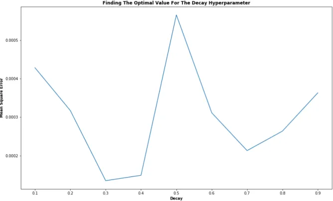
When using an optimizer there is an additional parameter that can be given to the optimizer that reduces the learning rate gradually when the network approaches optimal values. This additional parameter is called decay (Gers et al., 2000), we chose to use Adam as an opti-mizer because it was recommended to use as default (Stanford University) from fig. 10 we can see that the optimal value for the decay in our case is 0.3 because that value has the smallest MSE.

While doing this empirical test the dropout was set to 0.3, epoch to 380, the LSTM cells in each layer was set to 256, 256, 64 , 1 and the length of window to 22.

(22)

Figure 10: Illustrating empirical testing for finding the optimal value for Decay hyperparame-ter

3.5.5 Window

We then do an empirical test for finding the optimal length of a window, we do not want a to short window size because then the model will not acquire the longer dependencies hence neglecting important information. There is also a downside with a window size that is too large, it will then add a larger amount of redundant noise hence will overfit the training data (Graves and Schmidhuber, 2005). The best way to find the most suitable window size is to do an empirical test on diﬀerent window size (Gers et al., 2002) and find what value has the smallest MSE on the training data while training the LSTM model. From fig. 11 we can see that the optimal length for the window in our case is 45 training days.

While doing this empirical test the dropout was set to 0.3, epoch to 380, decay to 0.2, the LSTM cells in each layer was set to 256, 256, 256, 1.

(23)

Figure 11: Illustrating empirical testing for finding the optimal length for the window hyper-parameter

3.6 LSTM Loss Function

Loss function measures the distance between the LSTM model’s output and desired output during training for expedite learning. The desired output is the validation data that is set by the user, we have chosen to set the validation data to be 10% of the training data. This can then prevent overfitting by stopping the model when training because after each epoch the training data output is compared to the validation data. If the loss on the training is decreas-ing and at the same time the validation is increasdecreas-ing then we may be overfittdecreas-ing.

We have chosen the MSE as our loss function because it is widely used for time series forecast-ing when choosforecast-ing a loss function (Makridakis and Hibon, 1991).

3.7 LSTM Evaluation

For measuring the accuracy of predicting the S&P 500 price movement based on our trading strategy and LSTM model, we have set a side like describe before 10% of the trading days as the test data. We have normalized the adjusted closing price and that will be compared to the LSTM Models prediction when backtesting the test data. When backtesting the data we can see if the model that is build is overfitting (Bailey et al., 2016b), where this problem happens when the model is memorizing the data in our case adjusted closing price instead of learning the patterns (Stanford University).

3.7.1 Optimizer

When building the LSTM model we used the optimizer Adam because of its high performance and fast convergence compared to other alternative optimizer (Reimers and Gurevych, 2017)

(24)

and it was recommended to use it as default. When using the optimizer Adam we set the de-cay to 0.3.

3.7.2 Error Calculation

We then will evaluate the MSE and RMSE when evaluating the LSTM model’s train score and test score, where the score is the evaluation of our chosen loss function which in our case is MSE. The MAPE will also be calculated during the backtest of the data for ensuring that the model is predicting with high accuracy.

3.7.3 Measuring The Prediction 3.7.3.1 Hit Ratio

The accuracy of a model’s prediction can be measured with Hit ratio, where it is evaluated through this equation (Qiu and Song, 2016):

1 n n X n=1 pi (i = 1, 2, . . . , n) (8)

where pi denotes the prediction result on the ith _{trading day. The variable n is the number of} test data samples. The variable pi is defined by the equation:

pi = (

1, (yt+i yt)(ˆyt+i yˆt> 0)

0, Otherwise (9)

where yt denotes the actual adjusted closing price of the index at the ith _{trading day and ˆyt} _is the predicted adjusted closing price of the index at the ith _{trading day.}

3.7.3.2 Measurements

The accuracy of the backtesting will calculated with the hit ratio formula where we calculate the success of a prediction on the price movement based on our trading hence where our trad-ing strategy is based on a five day tradtrad-ing. But the hit ratio will only show us the accuracy of the model for predicting price movement. With a confusion matrix we can get a better un-derstanding of how our model is performing. The most common performance metric when evaluating the accuracy of a model are the metrics accuracy, precision, recall and F1-Score (Sokolova et al., 2006). We compare the model’s price movement prediction against the ac-tual price movement for a trading day, we can then classify those pairs as one out of these four comparison classification classes: True Positive, False Positive, True Negative and False Negative. The table below describes the confusion matrix classification.

Predicted Price Movement

Increase: Decrease: Actual Price

Movement Increase:Decrease: False Positive True NegativeTrue Positive True Negative Table 4: Confusion matrix for binary classification The comparison classification classes from the binary comparison are:

(25)

• True Positive is a correct positive price movement prediction. • False Positive is an incorrect positive price movement prediction. • True Negative is a correct negative price movement prediction. • False Negative is an incorrect negative price movement prediction.

Accuracy is a statistic measurement for how correctly a model predicts a price movement on a trading day corresponding to actual price movement on a trading day. The accuracy is the same as the hit ratio, the following equation describes how accuracy is calculated:

Accuracy =

P

(T rue P ositive) +P(T rue N egative) P

(T rue P ositive) +P(T rue N egative) +P(F alse P ositive) +P(F alse N egative) (10) Precision is the proportion between correctly predicted (positive) prediction in relation to all (positive) predictions. The following equation describes how precision is calculated:

P recision =

P

(T rue P ositive) P

(T rue P ositive) +P(F alse P ositive) (11) Recall describes the percentage of correctly predicted (positive) predictions that were identi-fied by the model, this evaluation is done by taking the fraction of (positive) predictions di-vided by all (positive) predictions. The following equation describes how recall is calculated:

Recall =

P

(T rue P ositive) P

(T rue P ositive) +P(F alse N egative) (12) F1 Score describes the harmonic between the recall and precision. The following equation de-scribes how F1-score is calculated:

F 1 Score = 2⇤ Recall ⇤ P recision

Recall + P recision (13)

3.7.4 Real Prediction

For measuring how accurate our LSTM model is we will make a prediction based on the past data to make prediction of the future history data. This will be done by feeding the LSTM model the last prediction that was feed to the LSTM model, which will be the last entry data of the training set, we will then make a prediction which will represent the next adjusted clos-ing price. We then save that predicted adjusted closclos-ing price which we can call P0 and start-ing to predict the next adjusted closstart-ing price by feedstart-ing P0 to the LSTM model we will get the predicted adjusted closing price P1. This iterative process will continue stepwise until we have predicted the number of trading days data as we want. When we then have predicted the price over a certain amount of trading days, we will plot the future price movement prediction for 5 trading day and the real adjusted closing price during that time. In this case we can see if our model has overfitted the data during the backtesting because if the plot of the predic-tion is not near the backtesting then we will know that our model has overfitted.

(26)

4 Results

4.1 Denormalized Prediction On Test Data

We denormalize the predicted adjusted closing price that we receive during the backtest with our LSTM model, the reason why we have to do that is because as describe earlier we had to normalize all input values to the LSTM model. In figure 12 we can see the LSTM model’s prediction for the adjusted closing price (red line) compared to the actual adjusted closing price (blue line).

(27)

4.2 MSE Loss

Figure 13 shows the training and validation loss of our LSTM model with optimal hyperpa-rameter setting, where the dropout is set to 30% and the decay of the optimizer Adam is set to 0.3. From the figure we can see that we are overfitting the data, the MSE loss does not de-crease for larger epoch values hence we can than see how the model starts to overfit the data heavily for larger epochs. The model does not learn any pattern or context instead is just memorize the training data we have. This will lead to that out validation loss will increase for longer epochs. The validation error is always larger then the training error which we try to avoid. This is a normal behavior when overfitting the data because the LSTM model has already seen the data during the training and the model was optimized for this training data.

Figure 13: MSE and RMSE Scores

4.3 Train And Test Score

Table 5 shows the obtained average MSE and RMSE values after evaluating the training and backtesting. We obtained the MAPE = 4.50574288% for our prediction accuracy of the model.

MSE RMSE

Train Score 2e-05 0.004 Test Score 0.00056 0.024

(28)

4.4 Absolute Percentage Error

Figure 14 displays the absolute percentage error of the prediction compared to the actual price. We can see compared to figure 5 that the largest percentage error for the prediction occurred on those trading days when the index was most volatile during that specific time pe-riod.

Figure 14: Absolute Percentage Error

4.5 Accuracy On Predicting The Test Data

Table 6 show the metrics obtained when backtesting our model with actual test data where we checked the price movement accuracy while using a trading strategy of trading every day in the end of the week hence after five trading days.

Index Accuracy/Hit Ratio Precision Recall F1-score

S&P 500 0.806 0.78 0.82 0.80

Table 6: Measurements Metrics

4.6 Real Prediction (No Backtesting)

Figure 15 shows the prediction made by the LSTM model on the price movement for 5 trad-ing days at a time when iteratively fed unseen data. We see that the prediction compared to backtesting is not even close. It shows the price movement right in some cases but in the other cases it is not even close.

(29)

(30)

5 Discussion

5.1 Discussion of the results

Our results have lead us to some interesting understandings. Initially our goal was to mea-sure the accuracy of LSTM to predict the stock market. To meamea-sure this accuracy we used a wide range of statistical models but most importantly we relied on the technique of backtest-ing that is seen as an industry standard in the scientific community when it comes to makbacktest-ing predictive models. Looking back at our findings in the result we first had a naive understand-ing of the workunderstand-ings of the LSTM algorithm when predictunderstand-ing data.

In figure 12, we ran our LSTM algorithm based on backtesting data. Our naive conclusion based on the accuracy measured during the backtest as table 6 show that our LSTM model has approximately 80% accuracy on predicting the adjusted closing price with a low training and test MSE & RMSE score as table 5 indicate. But as mentioned it is a naive conclusion to make that the LSTM can do an excellent prediction of the market, unknowing of the fact that the algorithm was converging towards a certain point and increasing the overfitting of the data as time progressed in the time series analysis as figure 13 indicates.

Our tests for accuracy using diﬀerent statistical measures such as the MSE loss and RMSE scores. In this case we were notified of the risk of overfitting and thus used an optimal hyper-parameter, however this did not help us. An issue might be that our hyperparameter was not optimized correctly. However, we used the conventional approach of optimizing a hyperparam-eter by looking at similar papers and using the MSE error for finding the most optimal hyper-parameter. There is also a risk of overfitting in the hyperparameter optimization, when one is looking back at the past data and running the MSE error function. There might be other more eﬃcient ways to approach this problem, but to highlight this is a crucial part of the re-sult to get the most optimized backtest rere-sult.

When looking at the absolute percentage error (figure 14) between our LSTM model’s pre-diction and the actual adjusted closing price we can see that the percentage error was larger when the S&P 500 adjusted closing price tended to be more volatile (figure 5). Just using an LSTM model will not help us to minimize the error during volatile periods of the index be-cause the volatility happens when e.g. during financial crisis or if some negative news concern-ing the index comes out to the public. Then the LSTM will not be able to predict with high accuracy. We would say that it is foolish to predict the adjusted closing price solely based on the open, high, low, close and adjusted closing price as input parameters when building a deep learning model. Financial markets are very complex and there are many factors involved in a stock/index price movement e.g. macro events, market noise, investor sentiment etc. also play an important part of the stock/index price.

In figure 15, we used the LSTM algorithm to make real predictions with no backtesting data. As the data shows the predictions did not performed well when feeding unseen data in a itera-tively process and this is by no means a prediction.

Looking at our results, there are two components that need more attention, the first is doing a more rigorous optimization of the hyperparameter and the second is an error in how we make the prediction. In the latter case the reason one can assume that there might be a problem in the prediction function is that the prediction is accelerating towards high values at a high pace, the function is not even attempting to predict even remotely close values.

(31)

5.2 Future Work

For future works in this field, there are several components that we believe other researchers should adopt to their frameworks of scientific work. The first part would be optimizing a hy-perparameter to deal with the problem of overfitting when backtesting the data. The second aspect of that would be to always do a prediction and compare that to the real time data. In-stead of just presenting backtested graphs in the paper. The third aspect would be to create a hybrid model where we use e.g. sentiment analysis to predict the volatility of the index price because we saw that the error of the prediction was larger when the index price tended to be volatile. We would then have considered more factors than just historical data about the price of the index.

(32)

6 Conclusion

The conclusion that we reached in this work was diﬀerent from the conclusion that we origi-nally had set out to achieve. I believe our conclusion is rather important and can assist other scientific works in this field, the field we refer to are the computational mathematics and com-putational finance where models are built and accuracy is measured for predictions. In the recent decade it has become almost a standard that a backtested data is a given and a mea-sure of accuracy. If one reads some papers written by other scientists in this field, one will be amazed by the overall high accuracy in all the models. Our conclusion leads us to question these results if they solely contain backtested data. Thus our recommendation is to always do a prediction based on real time data and measure that in complement with the backtested data results, because of the risk of overfitting. Even when deploying certain risk-management techniques to combat overfitting such as optimizing a hyperparameter we realized that overfit-ting is still present as a risk in the accuracy of the model.

(33)

References

David Bailey, Jonathan Borwein, Marcos Lopez de Prado, Amir Salehipour, and Qiji Zhu. Backtest overfitting in financial markets. 2016a.

David H Bailey, Jonathan M Borwein, Marcos Lopez de Prado, and Qiji Jim Zhu. The proba-bility of backtest overfitting. 2016b.

Jennifer Conrad and Gautam Kaul. An anatomy of trading strategies. The Review of Finan-cial Studies, 11(3):489–519, 1998.

Arnaud De Myttenaere, Boris Golden, Bénédicte Le Grand, and Fabrice Rossi. Mean absolute percentage error for regression models. Neurocomputing, 192:38–48, 2016.

Yahoo! Finance. S&P 500 (ˆGSPC), 2018. URL https://finance.yahoo.com/quote/ %5EGSPC/history/[Accessed:2018-03-11].

Felix A Gers, Jürgen Schmidhuber, and Fred Cummins. Learning to forget: Continual predic-tion with lstm. 1999.

Felix A. Gers, JÃÃrgen Schmidhuber, and Fred Cummins. Learning to forget: Continual pre-diction with lstm. Neural Computation, 12(10):2451–2471, October 2000. ISSN 0899-7667. Felix A Gers, Douglas Eck, and Jürgen Schmidhuber. Applying lstm to time series predictable

through time-window approaches. In Neural Nets WIRN Vietri-01, pages 193–200. Springer, 2002.

Ian J Goodfellow, David Warde-Farley, Mehdi Mirza, Aaron Courville, and Yoshua Bengio. Maxout networks. arXiv preprint arXiv:1302.4389, 2013.

Alex Graves and JÃrgen Schmidhuber. Framewise phoneme classification with bidirectional lstm and other neural network architectures. Neural Networks, 18(5):602–610, 2005. ISSN 0893-6080.

Alex Graves, Abdel-rahman Mohamed, and Geoﬀrey Hinton. Speech recognition with deep recurrent neural networks. March 2013.

David J Hand. Principles of data mining. Drug safety, 30(7):621–622, 2007.

Lawrence Harris. Sp 500 cash stock price volatilities. The Journal of Finance, 44(5):1155– 1175, 1989. ISSN 00221082, 15406261. URL http://www.jstor.org/stable/2328637. Sepp Hochreiter and Jürgen Schmidhuber. Long short-term memory. Neural computation, 9

(8):1735–1780, 1997.

Gareth James, Daniela Witten, Trevor Hastie, and Robert Tibshirani. An introduction to sta-tistical learning, volume 112. Springer, 2013.

Iebeling Kaastra and Milton Boyd. Designing a neural network for forecasting financial and economic time series. Neurocomputing, 10(3):215–236, 1996. ISSN 0925-2312.

Keras. Keras: The python deep learning library, 2018a. URL https://keras.io[Accessed: 2018-03-12].

(34)

Spyros Makridakis and MichÃle Hibon. Exponential smoothing: The eﬀect of initial values and loss functions on post-sample forecasting accuracy. International Journal of Forecasting, 7(3):317–330, 1991. ISSN 0169-2070.

Nasser M Nasrabadi. Pattern recognition and machine learning. Journal of electronic imaging, 16(4):049901, 2007.

Christopher Olah. Understanding lstm networks. 2015. URL http://colah.github.io/ posts/2015-08-Understanding-LSTMs/[Accessed:2018-03-19].

Mingyue Qiu and Yu Song. Predicting the direction of stock market index movement using an optimized artificial neural network model. PloS one, 11(5):e0155133, 2016.

Nils Reimers and Iryna Gurevych. Optimal hyperparameters for deep lstm-networks for se-quence labeling tasks. arXiv preprint arXiv:1707.06799, 2017.

Stuart J Russell and Peter Norvig. Artificial intelligence: a modern approach. Malaysia; Pear-son Education Limited„ 2016.

Jürgen Schmidhuber. Deep learning in neural networks: An overview. Neural networks, 61: 85–117, 2015.

Tanya Singh. How is artificial intelligence diﬀerent from ma-chine learning, 2017. URL https://www.linkedin.com/pulse/

how-artificial-intelligence-different-from-machine-learning-singh[Accessed: 2018-03-28].

Marina Sokolova, Nathalie Japkowicz, and Stan Szpakowicz. Beyond accuracy, f-score and roc: A family of discriminant measures for performance evaluation. In Abdul Sattar and Byeong-ho Kang, editors, AI 2006: Advances in Artificial Intelligence, pages 1015–1021, Berlin, Heidelberg, 2006. Springer Berlin Heidelberg. ISBN 978-3-540-49788-2.

Nitish Srivastava, Geoﬀrey Hinton, Alex Krizhevsky, Ilya Sutskever, and Ruslan Salakhutdi-nov. Dropout: A simple way to prevent neural networks from overfitting. The Journal of Machine Learning Research, 15(1):1929–1958, 2014.

Stanford University. Cs231n convolutional neural networks for visual recognition. URL http: //cs231n.github.io/neural-networks-3/[Accessed:2018-03-23].

Ilya Sutskever, Oriol Vinyals, and Quoc V Le. Sequence to sequence learning with neural net-works. In Advances in neural information processing systems, pages 3104–3112, 2014. Tensorflow. An open-source machine learning framework for everyone, 2018. URL https:

//www.tensorflow.org[Accessed:2018-03-12].

Cort J Willmott and Kenji Matsuura. Advantages of the mean absolute error (mae) over the root mean square error (rmse) in assessing average model performance. Climate research, 30 (1):79–82, 2005.

Wojciech Zaremba, Ilya Sutskever, and Oriol Vinyals. Recurrent neural network regulariza-tion. arXiv preprint arXiv:1409.2329, 2014.

(35)