DISSERTATION
ACTIVE RADIATION DETECTORS FOR USE IN SPACE BEYOND LOW EARTH ORBIT: SPATIAL AND ENERGY RESOLUTION REQUIREMENTS AND METHODS FOR HEAVY
ION CHARGE CLASSIFICATION
Submitted by Rafe A. McBeth
Department of Environmental and Radiological Health Sciences
In partial fulfillment of the requirements For the Degree of Doctor of Philosophy
Colorado State University Fort Collins, Colorado
Summer 2017
Doctoral Committee:
Advisor: Thomas Borak Alexander Brandl Andrew Ray
Copyright by Rafe A. McBeth 2017 All Rights Reserved
ABSTRACT
ACTIVE RADIATION DETECTORS FOR USE IN SPACE BEYOND LOW EARTH ORBIT: SPATIAL AND ENERGY RESOLUTION REQUIREMENTS AND METHODS FOR HEAVY
ION CHARGE CLASSIFICATION
Space radiation exposure to astronauts will need to be carefully monitored on future missions beyond low earth orbit. NASA has proposed an updated radiation risk framework that takes into account a significant amount of radiobiological and heavy ion track structure information. These models require active radiation detection systems to measure the energy and ion charge Z.
However, current radiation detection systems cannot meet these demands. The aim of this study was to investigate several topics that will help next generation detection systems meet the NASA objectives. Specifically, this work investigates the required spatial resolution to avoid coincident events in a detector, the effects of energy straggling and conversion of dose from silicon to water, and methods for ion identification (Z) using machine learning.
The main results of this dissertation are as follows: 1. Spatial resolution on the order of 0.1 cm is required for active space radiation detectors to have high confidence in identifying individual particles, i.e., to eliminate coincident events. 2. Energy resolution of a detector system will be limited by energy straggling effects and the conversion of dose in silicon to dose in biological tissue (water). 3. Machine learning methods show strong promise for identification of ion charge (Z) with simple detector designs.
ACKNOWLEDGEMENTS
I would like to thank Dr. Thomas Borak for allowing me to participate in his group at Colorado State University. Dr. Borak has forever changed my life and greatly contributed to my scientific development. He inspires me to be a better scientist and it has been a great honor to work with him over these years. I would also like to thank Dr. Alexander Brandl for always being there for me to talk with and for his very careful and thoughtful review of this dissertation. I also want to thank Dr. Thomas Johnson for his constant support over my graduate school career. He always found a way to help me, even when he told me he might not be able to. Finally, I would like to thank Dr. Susan LaRue for allowing me to work with her group in the Radiation Oncology Department at the CSU Veterinary Teaching Hospital. My time with Dr. LaRue confirmed and grew my passion for medical physics and I wouldn’t be on the path I am without her help.
A special thanks to my wife, Carly, who has stood by my side for all of this journey. We have built a beautiful family over these years and I will never forgot all the fun we had together in Fort Collins. To my daughter, Emery for always making me smile and laugh when I was at home, and to our newest addition Harlow for giving me strong motivation to finish this project before she arrived.
I would also like to thank my parents, Roger and Kathy, for their constant support over the years. You have always believed in my abilities and gave me the confidence to chase my dreams. To my extended family, you have all helped to mold who I am as a person in your own way. Although I often lose myself in my work, you are always in my thoughts and I’m thankful to have you in my life.
I am also very grateful to all the students and staff in the ERHS department that I have worked with over the years. You have all contributed to my growth in one way or another. I am particularly grateful for John Brogan and the friendship we have built over the years. Beating you at video games and basketball has always been great fun and a welcome distraction from hard work.
DEDICATION
To my amazing wife, Carly, for her unwavering support, it would have been impossible to complete this without you by my side. To my daughters, Emery and Harlow, being your dad will
TABLE OF CONTENTS
ABSTRACT . . . ii
ACKNOWLEDGEMENTS . . . iii
DEDICATION . . . iv
LIST OF TABLES . . . vii
LIST OF FIGURES . . . ix
Chapter 1 Introduction . . . 1
Chapter 2 Space radiation physical principles and protection . . . 7
2.1 Physical principles of radiation . . . 7
2.1.1 Fundamental Quantities . . . 7
2.1.2 Stopping power . . . 9
2.1.3 Linear Energy Transfer (LET) . . . 10
2.1.4 Nuclear fragmentation . . . 12
2.1.5 Energy straggling . . . 12
2.2 Biological effects of radiation . . . 14
2.3 Quality Factor and Radiation Protection . . . 15
2.4 Space Radiation Environment . . . 16
2.4.1 Solar Particle Event (SPE) . . . 17
2.4.2 Galactic Cosmic Rays (GCR) . . . 17
2.4.3 Radiation protection and quality factors for space . . . 18
2.5 Active radiation detectors . . . 22
2.6 Conversion of stopping power in silicon to stopping power in water . . . . 24
Chapter 3 Radiation transport methods and simulation designs . . . 26
3.1 Radiation Transport and Monte Carlo methods . . . 26
3.2 Geant4 Monte Carlo Toolkit . . . 27
3.2.1 Physics list selection . . . 28
3.2.2 Computer hardware and data size . . . 29
3.3 Simulation design . . . 29
3.3.1 General geometric setup . . . 30
3.3.2 Spectrum incident on shielding . . . 32
3.3.3 Particles tracked . . . 32
3.3.4 Idealized system . . . 33
3.3.5 Real detector system . . . 33
3.3.6 Particle identification system . . . 34
Chapter 4 Detector spatial resolution . . . 35
4.1 Detector spatial resolution analysis methods . . . 35
4.2 Detector spatial resolution results . . . 38
4.2.2 Stopping power distributions . . . 46
4.2.2.1 Ideal stopping power distributions . . . 46
4.2.2.2 Coincident stopping power distributions . . . 54
4.3 Spatial resolution conclusions . . . 61
Chapter 5 Detector energy resolution . . . 62
5.1 Detector energy resolution methods . . . 62
5.2 Detector energy resolution results . . . 64
5.2.1 Distributions of stopping power in real detectors . . . 64
5.2.2 Stopping power conversion results . . . 69
5.3 Energy resolution conclusions . . . 72
Chapter 6 Ion classification with machine learning . . . 73
6.1 Introduction . . . 73
6.2 Background . . . 73
6.2.1 Machine learning in radiation detection . . . 74
6.3 Machine learning methods . . . 75
6.3.1 Machine learning algorithm . . . 77
6.4 Results . . . 77
6.4.1 Data set basics . . . 78
6.4.2 Single detector machine learning . . . 79
6.4.3 Dual detector machine learning . . . 84
6.5 Machine Learning Conclusions . . . 86
Chapter 7 Conclusion . . . 93
LIST OF TABLES
2.1 ICRP 26, 1977, Quality factor as a function of LET1 . . . 15 2.2 ICRP 60, Quality factors as a function of LET1 . . . 16 2.3 Career whole body dose equivalent limits based on a lifetime excess risk of cancer
mortality of 3 ⇥ 10 2 . . . 19 2.4 Short term dose equivalent and career limits for protection against non-stochastic
ef-fects (Sv) to the blood forming organs (BFO), lens of the eye and the skin. . . 20 3.1 Geant4 simulation settings: range cuts and energy production thresholds for various
particles in water and silicon . . . 29 4.1 Dose mean stopping power [keV/µm] in silicon and water for incident He ions of
varying energies. 5.4 g/cm2, 13.5g/cm2, 54 g/cm2 Al shielding and 10 cm downstream 48 4.2 Dose mean stopping power [keV/µm] in silicon and water for incident C ions of
vary-ing energies. 5.4 g/cm2, 13.5g/cm2, 54 g/cm2Al shielding and 10 cm downstream . . . 50 4.3 Dose mean stopping power [keV/µm] in silicon and water for incident silicon ions of
varying energies, 5.4 g/cm2, 13.5g/cm2and 54 g/cm2Al shielding and 10 cm downstream 52 4.4 Dose mean stopping power [keV/µm] in silicon and water for incident Fe ions of
vary-ing energies. 5.4 g/cm2, 13.5g/cm2, 54 g/cm2Al shielding and 10 cm downstream . . . 52 4.5 Dose mean stopping power [keV/µm] in Si for the ideal, 5 cm pixel and 0.1 cm pixel
cases for incident He ions of varying energies. 5.4 g/cm2, 13.5g/cm2, 54 g/cm2 Al shielding and 10 cm downstream . . . 56 4.6 Dose mean stopping power [keV/µm] in silicon for the ideal, 5 cm pixel and 0.1 cm
pixel cases for incident C ions of varying energies. 5.4 g/cm2, 13.5g/cm2, 54 g/cm2Al shielding and 10 cm downstream . . . 56 4.7 Dose mean stopping power [keV/µm] for incident Si ions for the ideal, 5 cm pixel and
0.1 cm pixel cases in silicon of varying energies. 5.4 g/cm2, 13.5g/cm2, 54 g/cm2 Al shielding and 10 cm downstream . . . 59 4.8 Dose mean stopping power [keV/µm] for incident Fe ions for the ideal, 5 cm pixel and
0.1 cm pixel cases in silicon of varying energies. 5.4 g/cm2, 13.5g/cm2, 54 g/cm2 Al shielding and 10 cm downstream . . . 61 5.1 Dose mean stopping power [keV/µm] in silicon for the ideal and real case for incident
helium ions of varying energies after 5.4 g/cm2, 13.5g/cm2, 54 g/cm2 Al shielding. The physical detector system is 10 cm downstream from the back of the shielding . . . 66 5.2 Dose mean stopping power [keV/µm] in silicon for the ideal and real case for incident
carbon ions of varying energies after 5.4 g/cm2, 13.5g/cm2, 54 g/cm2 Al shielding. The physical detector system is 10 cm downstream from the back of the shielding . . . 66 5.3 Dose mean stopping power [keV/µm] in silicon for the ideal and real case for incident
silicon ions of varying energies after 5.4 g/cm2, 13.5g/cm2, 54 g/cm2Al shielding. The physical detector system is 10 cm downstream from the back of the shielding . . . 69
5.4 Dose mean stopping power [keV/µm] in silicon for the ideal and real case for incident iron ions of varying energies after 5.4 g/cm2, 13.5g/cm2, 54 g/cm2 Al shielding. The physical detector system is 10 cm downstream from the back of the shielding . . . 69 5.5 Table of mean stopping power ratio, stopping power in water over stopping power in
silicon for the various shielding thicknesses simulated . . . 72 6.1 Performance summary of the machine learning algorithm for the single detector case. . 90 6.2 Performance summary of the machine learning algorithm for the two detector system. . 91
LIST OF FIGURES
2.1 Graphical representation of the quality factor as defined by the ICRP 26 (Table 2.1) and ICRP 60 (Table 2.2). Quality factor is shown as a function of unrestricted LET, LET1. Adapted from ICRP 92 Figure 1.1 (ICRP, 2003) . . . 16 2.2 Galactic Cosmic Radiation (GCR) spectrum in free space. The abscissa of the plot
is the ion charge Z ranging from proton (Z = 1) to Iron (Z = 26). The ordinate is the energy of the ions in MeV per nucleon. The colors represent the fluence rate of particles. . . 18 2.3 Contribution of absorbed dose from Galactic Cosmic Radiation (GCR) spectrum in
free space. The abscissa of the plot is the ion charge Z ranging from proton (Z = 1) to Iron (Z = 26). The ordinate is the energy of the ions in MeV per nucleon. The colors represent the contribution to radiation dose. Note, the units for this plot are a surrogate for radiation dose and are not converted to J/kg in tissue. . . 19 2.4 Contribution of dose equivalent from Galactic Cosmic Radiation (GCR) spectrum in
free space. The abscissa of the plot is the ion charge Z ranging from proton (Z = 1) to Iron (Z = 26). The ordinate is the energy of the ions in MeV per nucleon. The colors represents the contribution to radiation dose equivalent. Note, the units for this plot are a surrogate for radiation dose equivalent and are not converted to the unit of Sv. . . 21 3.1 Geometric setup for experiment showing ion normally incident on shielding material
with detector downstream. The detector segmentation and size shown are representa-tive and were not used in the final design, discussed later in this paper. . . 30 3.2 Inverse cumulative flux of GCR ions in free space. Based on the Badhwar-O’neill
2010 GCR model. Solar minimum and solar maximum values are based on 2010 and 2001 solar cycle respectively. Vertical dashed lines show the energy selections for this project. Horizontal dashed lines show the 75, 50 and 25 percentile. . . 32 4.1 Proximity matrix flow chart: A matrix of distances between particles is created. The
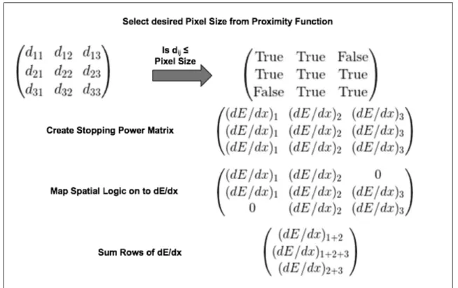
diagonal vector of the matrix is always zero and the lower triangle is taken to remove duplicate events. The resultant matrix is then used to create the proximity and inverse cumulative distributions. . . 37 4.2 Coincident matrix flow chart: A matrix of each particle from its neighboring particles
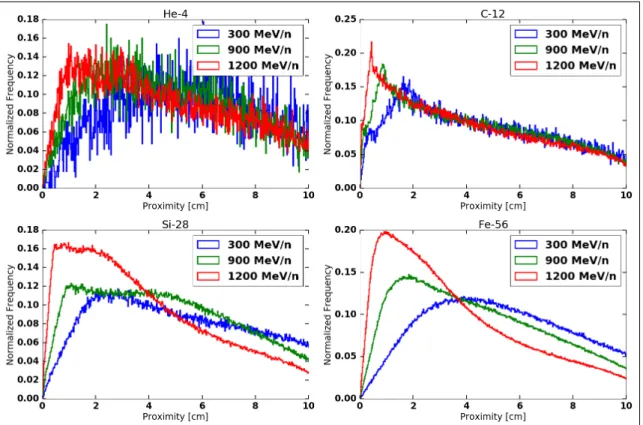
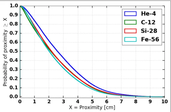
is created. A truth matrix is then created based on the selected pixel size. The truth matrix mask is applied to stopping power matrix. The result is then summed across the rows to get the coincident stopping power values. . . 38 4.3 Proximity distributions: 5.4 g/cm2 of aluminum shielding at 10 cm downstream from
the back of the shield for incident He-4, C-12, Si-28 and Fe-56. . . 40 4.4 Proximity distributions: 5.4 g/cm2 of aluminum shielding at 20 cm downstream from
the back of the shield for incident He-4, C-12, Si-28 and Fe-56. . . 41 4.5 Inverse cumulative proximity distribution for all incident ions at 10, 20 and 50 cm
4.6 Inverse cumulative proximity distribution for all incident ions at 10, 20 and 50 cm downstream after 5.4 g/cm2 (2 cm) of Al shielding. This plot focuses on the small pixel size and high probability region. . . 43 4.7 Inverse cumulative proximity distribution 10 cm downstream for each ion after 5.4
g/cm2 (2 cm) of Al shielding. . . 43 4.8 Inverse cumulative proximity distribution 10 cm downstream for each ion after 5.4
g/cm2 (2 cm) of Al shielding. This plot focuses on the small pixel high probability region. . . 44 4.9 Proximity distribution 10 cm downstream after 54 g/cm2(20 cm) of Al shielding. . . . 44 4.10 Inverse cumulative proximity distribution for all incident ions 10 cm downstream 5.4
g/cm2, 13.5 g/cm2, 54 g/cm2 of Al shielding . . . 45 4.11 Zoomed in inverse cumulative proximity distribution for all incident ions 10 cm
down-stream 5.4 g/cm2, 13.5 g/cm2, 54 g/cm2of Al shielding . . . 45 4.12 Stopping power in Si distribution for incident He ions of 300, 900 and 2400 MeV/n
after 5.4 g/cm2, 13.5 g/cm2, 54 g/cm2of Al shielding . . . 47 4.13 Stopping power in Si distribution for incident C ions of 300, 900 and 2400 MeV/n after
5.4 g/cm2, 13.5 g/cm2, 54 g/cm2 of Al shielding . . . 49 4.14 Stopping power in Si distribution for incident Si ions of 300, 900 and 2400 MeV/n
after 5.4 g/cm2, 13.5 g/cm2, 54 g/cm2of Al shielding . . . 51 4.15 Dose mean stopping power [keV/µm] in silicon and water for incident iron ions of
varying energies, 5.4 g/cm2, 13.5g/cm2and 54 g/cm2Al shielding and 10 cm downstream 53 4.16 Stopping power distributions is Si for 5 cm pixel vs ideal for incident He ions of 300,
900 and 2400 MeV/n after 5.4 g/cm2, 13.5 g/cm2, 54 g/cm2 of Al shielding . . . 55 4.17 Stopping power distributions is Si for 5 cm pixel vs ideal for incident C ions of 300,
900 and 2400 MeV/n after 5.4 g/cm2, 13.5 g/cm2, 54 g/cm2 of Al shielding . . . 57 4.18 Stopping power distributions is Si for 5 cm pixel vs ideal for incident Si ions of 300,
900 and 2400 MeV/n after 5.4 g/cm2, 13.5 g/cm2, 54 g/cm2 of Al shielding . . . 58 4.19 Stopping power in Si distribution for incident Fe ions of 300, 900 and 2400 MeV/n
after 5.4 g/cm2, 13.5 g/cm2, 54 g/cm2of Al shielding . . . 60 5.1 Results from initial simulation to verify energy straggling effects and physics package
selection. These plots show the 4 ions and 3 energies used in the simulations incident on a 300 µm detector. No shielding was used before the detector in these cases. Bethe-Bloch and the mean of the distribution are also plotted for reference. . . 63 5.2 Distributions of stopping power in silicon for incident helium ions of 300, 900 and
2400 MeV/n after 5.4 g/cm2, 13.5 g/cm2, 54 g/cm2 of Al shielding. The ideal stopping power as measured by a virtual detector are plotted along with the stopping power measured in a real detector. . . 65 5.3 Distributions of stopping power in silicon for incident carbon ions of 300, 900 and
2400 MeV/n after 5.4 g/cm2, 13.5 g/cm2, 54 g/cm2 of Al shielding. The ideal stopping power as measured by a virtual detector are plotted along with the stopping power measured in a real detector. . . 67
5.4 Distributions of stopping power in silicon for incident silicon ions of 300, 900 and 2400 MeV/n after 5.4 g/cm2, 13.5 g/cm2, 54 g/cm2 of Al shielding. The ideal stopping power as measured by a virtual detector are plotted along with the stopping power measured in a real detector. . . 68 5.5 Distributions of stopping power in silicon for incident iron ions of 300, 900 and 2400
MeV/n after 5.4 g/cm2, 13.5 g/cm2, 54 g/cm2 of Al shielding. The ideal stopping power as measured by a virtual detector are plotted along with the stopping power measured in a real detector. . . 70 5.6 Histogram showing the frequency of the ratios of stopping power in water vs silicon . . 71 6.1 These two plots highlight the challenges a machine learning algorithm will face when
trying to identify ions based on stopping power. The stopping power of six ions, based on the Bethe-Bloch formalism, are plotted as a function of energy in MeV/n. The dashed line is representative of a single measurement of stopping power. The plot on the left shows how an ideal detection system may identify the particle species based on stopping power. The plot on the right shows the challenges in identification when energy straggling is present. . . 75 6.2 Histogram showing the normalized frequency of ion charge distribution used in these
studies. In this plot the normalized frequency is plotted on a linear scale. . . 78 6.3 Histogram showing the normalized frequency of ion charge distribution used in these
studies. In this plot the normalized frequency is plotted on a logarithmic scale. . . 79 6.4 Scatter plot of the stopping power of individual particles in the detector with their
associated ion charge. The opacity of the markers has been reduced to 1% of normal. This highlights the most densely populated areas of the plot and helps to reduce the prevalence of outliers. . . 80 6.5 Confusion matrix for the one detector case. This plot shows the normalized percentage
of classification with the predicted classification on the vertical axis and the actual classification on the horizontal axis. . . 81 6.6 Histogram of the difference between the actual Z values and the predicted values. The
frequency of events is normalized and the vertical axis is on a log scale. . . 83 6.7 Scatter plot of the stopping power of individual particles in each detector. The
stop-ping power measured in the first detector is plotted along the vertical axis. While the stopping power measured in the second detector is plotted along the horizontal axis. The color of each point represents the ion charge Z. The opacity of the markers has been reduced to 1% of normal and a color based on the ion charge has been added. . . 85 6.8 Confusion matrix for the two detector case. This plot shows the normalized percentage
of classification with the actual classification on the horizontal axis and the predicted classification on the vertical axis. . . 86 6.9 Histogram of the difference between the true Z value and the predicted values for the
two detector case. The frequency of events is normalized and the vertical axis is on a log scale. . . 87 6.10 Machine learning algorithm precision plotted as a function of ion charge for the one
and two detector case. Precision was increased without exception from the one detector case to the two detector case. . . 88
6.11 Machine learning algorithm recall plotted as a function of ion charge for the one and two detector case. Recall was increased without exception from the one detector case to the two detector case. . . 89 6.12 Machine learning algorithm f1score plotted as a function of ion charge for the one and
two detector case. The f1 score was increased without exception from the one detector case to the two detector case. . . 92
Chapter 1
Introduction
Long duration missions in space, such as a mission to Mars, will expose astronauts to radiation from high energy (E > 20 MeV/n) and high atomic number (Z 2) heavy ions (HZE) at historically high levels. Heavy ion radiotherapy is also being used increasingly to treat malignant tumors using a subset of HZE particles. As these ions pass through materials, they deposit energy in complex ways. Radiation detection systems that accurately measure HZE ions to determine radiation dose to astronauts or patients are essential for future space missions and the expansion of heavy ion therapy treatments. In fact, NASA has defined the development of a compact radiation detector capable of determining energy and charge of incident radiation as a major technical challenge for future manned space missions (Hurlbert et al., 2012).
The radiation environment in space is composed of two major components, solar particle events (SPE) and galactic cosmic rays (GCR). SPE are composed of 98% protons, 1% helium and 1% other HZE ions and their flux can vary significantly over time. GCR are composed of 87% protons, 12% helium ions and 1% HZE ions. GCR orginate from outside the solar system and will be omnidirectionally incident on astronauts. While the fluence of ions in space with charge Z > 2 is only 1% of the GCR spectrum, these high Z ions contribute significantly to the radiation dose. The high Z ion component of the radiation environment in space is the primary focus of this study.
As heavy ions travel through a medium they transfer energy primarily through electromagnetic interaction. Ionization and excitation are the two main electromagnetic processes by which space radiation loses energy. Ionization occurs when an incident heavy ion transfers sufficient energy to strip an orbiting electron from an atom or molecule in a material. Energy transferred below the threshold for ionization excites the atom or molecule in the target material and can lead to subse-quent de-excitation. For HZE ions, nuclear (strong force) interactions with the nuclei of the target material are also possible. Nuclear interactions produce many secondary fragments that originate
teraction is low, when compared to electromagnetic interaction, the effects of fragmentation on the radiation field can be significant. In hadron radiation therapy applications, up to 80% of an incident carbon ion beam has fragmented by the time it reaches a depth of 10 cm in water (McBeth and Borak, 2015). For space applications, Le Tessa et al. found that 68% of a 1 GeV/nucleon iron beam has fragmented after 9.6 cm of aluminum (La Tessa et al., 2005).
HZE ions are believed to have qualitatively and quantitatively different effects on biologi-cal systems when compared to the natural radiation background found on earth (Durante, 2014). Moreover, less information is available about the effects that space radiation has on humans due to the small number of individuals exposed. An important risk to astronauts from space radiation is the induction of cancer. Non-cancer effects, such as damage to the central nervous system (CNS) and late cardiovascular disease are of increasing concern and have large uncertainties in the esti-mated risk (Durante and Cucinotta, 2008). Data also suggest that heavy ions cause damage through non-targeted effects (Durante, 2012). The assessment of radiation risk for both acute and late ef-fects, will be essential for ensuring the health and safety of astronauts. The National Committee on Radiation Protection (NCRP) and NASA have published many documents on the appropriate methods for radiation protection in space (Cucinotta et al., 2013; NCRP, 1989, 2002, 2006, 2014). Radiation protection in space is focused on ensuring short and long term effects of radiation are limited to acceptable levels. A quality factor, Q, is a factor that modifies the absorbed radiation dose based on biological effectiveness, and is an important concept in radiation protection. His-torically Q has depended on the measured spectra of linear energy transfer (LET). In preparation for space missions beyond low earth orbit, significant efforts have been directed towards updating quality factors to more accurately reflect the biological damage HZE particles cause (Cucinotta et al., 2013). This revised quality factor, QNASA, requires future detection systems to not only measure the LET but also the charge Z and velocity of HZE ions. However, detector systems deployed into space have a limited ability to measure individual particle charge and velocity, and do not provide sufficient information for the accurate determination of radiation risk to astronauts under the new NASA paradigm.
To meet the requirements of the new NASA quality factor, future detection systems will need to have appropriate spatial resolution to ensure properties of individual particles, such as LET or the charge Z, are correctly identified. In practice, the spatial resolution of a detection system will be defined by the segmentation or pixelation of the detector e.g., a detector with a pixel size of 1 cm will also have a spatial resolution of 1 cm. Coincident events from the primary GCR spectrum are rare, due to the low fluence, but secondary projectile fragments emerge from shielding with similar velocities and are grouped in space and time. Grouped particles intercepting a radiation detector simultaneously will register the sum of the energy deposition, introducing errors into the measured energy spectrum. A detection system must have the spatial resolution capable of ensuring that only single heavy ion events are recorded. The ability of a detector to identify individual particles will be defined as the spatial resolution in this paper.
A radiation detector with sufficient spatial resolution to measure individual particles will also require sufficient energy resolution. Detection systems that use thin silicon radiation detectors, such as the Radiation Assessment Detector (RAD) currently mounted on the Mars Curiosity rover and the detector system evaluated in this study, will have limited energy resolution. This lim-ited energy resolution is due to the statistical variation in energy deposlim-ited as a heavy ion passes through a thin detector. Although small energy transfers in a thin detector are most common, in-frequent large energy transfers can result in significant energy loss and add large uncertainty to the determination of particle stopping power. This phenomenon is referred to as energy straggling. Energy straggling will limit the ability of a detector to identify a particles’ charge (Z) and velocity ( ) as required by the NASA quality factor.
In addition to spatial and energy resolution of a detector system, conversion of measured energy deposition in a detector to biologically relevant materials must be considered. Specifically, a silicon radiation detection system that measures stopping power will have to be converted to stopping power in water. Historically, radiation detection systems have used a single factor to scale stopping power in Si to LET in water (Zeitlin et al., 2013). Uncertainties that result from this conversion will propagate to the dose, dose equivalent values and ultimately assessment of risk.
To investigate the spatial resolution, energy resolution, and stopping power conversion factors required, experiments were simulated using Monte Carlo radiation transport methods. For these studies a subset of the space radiation spectrum, specifically He, C, Si, and Fe, were directed at aluminum shields of varying thickness, 2, 5, and 10 cm. To investigate the spatial resolution required for detectors used beyond low Earth orbit, a idealized detector system with a virtual detector was used, while a physical detector system, using a 300 µm silicon real detector, was used for the study of energy resolution and stopping power conversion factors.
A virtual detector in this context is a plane downstream from the shielding that scores the pri-mary and fragment ions as they intercept the plane, but do not interact with the particles. Incident ions are directed normally at the shield and the position of the transmitted are recorded as they in-tercept the virtual detector. A novel analysis method, leading to proximity distributions, was used to evaluate the data and determine what spatial resolution requirements are necessary to satisfy the demands of the mission. Proximity distributions provide the probability that more than one particle will intercept the same pixel for a given pixel size. These distributions can then be used to determine the pixel size necessary to achieve a desired level of confidence in measuring individ-ual particles. The stopping power distributions of the virtindivid-ual detector system and an unsegmented detector system are presented to assess the impact that coincident events may have had on non pixelated detectors in the past.
The next step was to investigate the effects of energy straggling, assuming the detection system is appropriately segmented. Simulations were performed with a physical detector system, i.e., a 300 µm thin silicon real detector. Stopping power distributions are created that show the difference between the idealized detector system and the physical detector system, with energy straggling. Additionally, metrics such as the dose mean stopping power are compared to evaluate the difference between an ideal detection system and a real detection system. Energy straggling in a thin detector system cannot be mitigated. Thus, a thorough understanding of energy straggling will be necessary for the identification of the distribution of Z and in the radiation environment.
The next goal of this work was to determine if it is possible, using the simplistic detector design of the energy straggling studies, to accurately identify the charge Z of ions in the radiation environment. To do this, methods of the fast growing field of machine learning were used. A machine learning algorithm is a computational process that attempts to "learn" how to achieve the desired goal. These algorithms emulate human intelligence by learning from its surroundings and have become crucial in the era of "big data". These techniques have been successfully applied to self-driving cars, robot tasks, pattern recognition, computer vision, finance, computational biology, and medical applications. In this paper, we present applications of machine learning techniques to the problem of ion classification.
To summarize, this paper provides results for four main questions about the general charac-teristics a detection system will need to identify Z, , and the linear energy transfer of individual particles that contribute to space radiation dose. The questions are:
1. What spatial resolution (pixel size) is required for a radiation detection system to have high confidence that only one heavy ion is measured?
2. To what extent does energy straggling change the measurement of stopping power spectra? 3. Is a single scaling factor appropriate for converting stopping power in a Si detector to
stop-ping power in water?
4. Is it possible to use machine learning techniques to identify the charge Z of individual par-ticles using a simplistic radiation detection system?
Outline of Dissertation
• The basic principles of radiation interaction and the fundamentals of radiation protection are discussed in Chapter 2. These sections also introduce radiation detection methods that have been used in previous missions.
• Simulation output analysis methods and results for the determination of optimum radiation detector pixel size are discussed in Chapter 4.
• Energy resolution for a basic detection system is analyzed in Chapter 5. This includes how energy straggling affects estimates of LET, and issues that arise from the conversion of stopping power in silicon to stopping power in water.
• Machine learning methods for ion classification, i.e., identification of Z, are discussed in Chapter 6.
Chapter 2
Space radiation physical principles and protection
2.1 Physical principles of radiation
As radiation interacts with a medium, it can lose energy in numerous ways depending on the type of incident radiation. X, , and heavy ion radiation transfer energy to the medium by the process of excitation and ionization. Ionization is the removal of bound electrons from the target atoms or molecules. Excitation is process of the incident radiation imparting energy on an atom or molecule and leaving it in a excited state.
Ionization can be indirect or direct. Indirect ionization occurs when non charged radiation, such as photons and neutrons, liberate charged particles such as electrons. It is also possible for these ionized electrons to create their own ionizations. When electrons act as ionizing particles they are often called delta rays. Charged particles such as electrons, protons, alpha particles, and heavier nuclei are directly ionizing. The rate at which heavy charged particles lose energy per unit length (dE/dx) is the stopping power (S), and is discussed in detail in Section 2.1.2. Linear energy transfer (LET) is related to stopping power but has the distinct difference that it is a measure of the energy absorbed in a medium, not the energy lost by the particle, as in the definition of stopping power. LET is discussed in more detail in Section 2.1.3.
2.1.1 Fundamental Quantities
Several fundamental quantities have been defined to quantify the physical nature of radiation. Quantities have also been developed to quantify how radiation interacts with a medium such as human tissue.
The amount of radiation incident on an object is described using the fluence. Fluence, , is defined as:
= dN
Where dN is the number of particles incident on a sphere of cross-sectional area da and the unit is often given in particles cm 2 (ICRU, 1993). The rate at which particles are incident is the fluence rate and is the fluence of particles per unit time,
˙ = dt =
dN
dadt, (2.2)
where dt is a unit time, such as 1 hour. The unit of fluence rate is particles cm 2s 1.
Over the years, methodologies to describe the effects of radiation and the associated risk have been developed. Two fundamental ideas are the constructs of absorbed dose and dose equivalent.
Absorbed dose is a fundamental concept of radiation dosimetry and is a measure of the amount of energy imparted to a medium by all types of radiation. The absorbed dose, D, is defined as the average energy absorbed per unit mass of a target for ionizing radiation (ICRU, 2011). The SI unit for absorbed dose is J kg 1 and has the special name gray (Gy) or the traditional name rad. The relationship between gray (Gy) and rad is
1 Gy = 100 rad. (2.3)
Absorbed dose is a point function, has a value at every position in an irradiated volume and is the quotient of d¯✏ by dm,
D = d¯✏
dm, (2.4)
where d¯✏ is the mean energy imparted by ionizing radiation to matter of mass dm (ICRU, 1993). Alternatively, the absorbed dose can be written as
D = ·LET
⇢ , (2.5)
where is the fluence, LET is the linear energy transfer of the ion, and ⇢ is the density of the medium. In this alternative form, the units in the equation need to be appropriately converted to
Dose equivalent, H, is an additional construct that takes into account the fact that some particles are more damaging and have higher associated risk than the standard radiation, 200 keV photons. Dose equivalent is defined as the product of absorbed dose, D, and a dimensionless quality factor Q,
H = D· Q. (2.6)
The concept of dose equivalent is applicable only to human beings and has the same physical di-mensions as absorbed dose, J kg 1, but has the different SI unit of the sievert (Sv) or the traditional unit rem. The relationship between sievert (Sv) and rem is
1 Sv = 100 rem (2.7)
The quality factor and associated radiation protection limits will be discussed in more detail in Section 2.3.
2.1.2 Stopping power
Hadrons, such as the heavy ions found in GCR, lose their energy primarily by Coulomb force interaction (ionizations and excitations) but also have the potential to have nuclear reactions. The rate at which heavy charged particles lose energy per unit length (dE/dx) by interaction with electrons of the medium is defined as the stopping power (S) and to a first approximation is given by the Bethe-Bloch equation:
S = dE dx = 4⇡k2 0Z2e4n mc2 2 2mc2 2 I(1 2) 2 . (2.8)
In equation 2.8
k0 = 8.99⇥ 109N m2C 2,
Z =atomic number of heavy ion, e =electron charge,
n =electrons per unit volume of medium, m =electron rest mass,
c =speed of light in vacuum,
= V /c =speed of particle relative to c I =mean excitation energy of the medium
Equation 2.8 shows that the stopping power is dependent on the velocity ( ) and charge (Z) of the incident ion and the properties of the medium. Equation 2.8 considers the energy lost by ionization but does not consider nuclear interactions.
2.1.3 Linear Energy Transfer (LET)
Linear energy transfer (LET) is distinctly different from stopping power discussed in Section 2.1.2. While stopping power is the energy lost by the particle as it travels through a medium, dE/dx, LET can be considered as the energy absorbed by the medium. Original definitions of LET only considered the radiation absorbed within a specific radial distance or maximum electron energy. This definition of LET excluded the contribution of delta rays that deposit dose at a distance from the central track of a heavy ion. For large volumes where these secondary high energy delta rays (electrons) are fully absorbed, LET and stopping power are equivalent. In smaller volumes, such as biological cells, the difference between the energy lost by an incoming ion and the energy deposited in the small volume can be significant. Additionally, similar to stopping power, the LET is considered to be an averaged quantity at a point, and thus is not representative of statistical fluctuations in the deposited energy.
LET or linear energy transfer is generally defined as the energy transferred per unit path length of the track. However the definition has undergone subtle changes over the years. The 1970 ICRU report no. 16 titled Linear Energy Transfer ICRU (1970) defined it as:
The linear energy transfer or restricted linear collision stopping power (L ) of charged particles in a medium is the quotient of dE by dl, where dl is the distance traversed by the particle and dE is the mean energy-loss due to collisions with energy transfers less than some specified value .
L = ✓
dE dl
◆
ICRU Report 85a (ICRU, 2011) defines the linear energy transfer or restricted linear electronic stopping power, L , of a material as
L = dE dl .
Where dE is the mean energy lost by the charged particles due to electronic interactions in traversing a distance dl, minus the mean sum of the kinetic energies in excess of of all the electrons released by the charged particles. This can also be written as
L = Sel
dEke, dl ,
where Sel is the linear electronic stopping power, and dEke, is the mean sum of the kinetic ener-gies, greater than , of all the electrons released by the charged particle in traversing a distance dl. It is important to note that the binding energies for all collisions are included in the definition. ICRU report 85a further describes the energy balance as:
Energy lost by the primary charged particle in interactions with electrons, along a distance dl, minus the energy carried away by energetic secondary electrons hav-ing initial kinetic energies greater than , equals energy considered as “locally
trans-The unrestricted LET, L1, is the linear energy transfer considering no energy cutoff. This is equivalent to the electronic stopping power. LET is used to determine the quality or effectiveness of radiation in the human body and is a dependent variable in the concept of Relative Biological Effectiveness (RBE).
2.1.4 Nuclear fragmentation
High energy ions have sufficient energy to overcome Coulomb forces and interact with the nucleus of target material atoms. The nuclear cross section for these interactions is small and negligible in thin materials. However, for thick materials, such as space craft, habitat shielding, or patients in heavy ion therapy, nuclear reactions cannot be ignored. Nuclear fragmentation is the process by which heavy ions interact with a medium and produce secondary nuclei (fragments). Fragments can originate from both the incident ion and the target material. These fragments will be grouped temporally and spatially.
Fragments simultaneously impacting a detection system will register as a single event and distort the resultant distributions of stopping power and estimates of risk. Future detection systems should be designed to eliminate these simultaneous or coincident events and accurately measure individual particles.
2.1.5 Energy straggling
As described in Section 2.1.2, stopping power is an averaged quantity and does not include the statistical fluctuations in energy lost. For thick absorbers, the variation in energy loss can be described by a symmetric distribution. In thin absorbers, where the energy lost in the material is small in comparison to the total energy of the incident particles, the distribution can be highly skewed. The energy lost in a collision with a single electron, ✏, is proportional to 1/✏2. This implies that small energy transfers are far more common than large energy transfers. Although large energy transfers are infrequent, they can account for a large proportion of the total energy loss.
There are several theories that describe the probability distribution of energy loss when heavy charged particles pass through a thin absorber. The various theories for energy straggling are summarized well in a paper by Maccabee et al. (Maccabee et al., 1968). When the the number of collisions of a heavy ion in an absorber is large, i.e., a thick absorber, Bohr showed that the energy loss probability distribution is Gaussian (Bohr, 1915). The mean of this distribution is given by the Bethe-Bloch function, Equation 2.8 of Section 2.1.2. The variance for this Gaussian distribution is given by
2 = 4⇡e4Z2N zx, (2.9)
where e is the electron charge, Z is the incident heavy ion charge number, N is the number of atoms/cm3 of the absorber material, z is the atomic number of the material and x is the absorber thickness. Equation 2.9 is appropriate when the number of energy deposition events in each possi-ble energy range is large. Mathematically Equation 2.9 is valid when
⇠/✏max>> 1, (2.10)
where
⇠ = 2⇡e4Z2N zx/mv2, (2.11)
and m is the electron mass, v is the particle velocity and ✏max is the maximum possible energy transfer in a heavy ion-electron collision. Non-relativistically the maximum possible energy a heavy ion can transfer to an electron is
✏max= 2mv2/(1 2), (2.12)
where = v/c.
The opposite case is when the number of collisions in the highest energy range is small, i.e.,
Landau solved this case in 1944 and showed that the probability distribution of energy losses is highly asymmetric with a broad peak around the most probable energy loss and a long tail (Landau, 1944). The full width at half-maximum (FWHM) was given as
F W HM = 3.98⇠. (2.14)
In these cases the most probable energy loss, mp, is much lower than the average energy loss, av, given by Bohr. The most probable energy loss is given as
mp= ⇠ln[2mv2⇠/I2(1 2)] 2+ 0.37, (2.15)
where I is the mean excitation potential of the material. For reference, the mean excitation relevant to this work are 75 eV for water and 173 eV for silicon.
Vavilov treated the case in between Landau and Bohr in 1957 (Maccabee et al., 1968; Vavilov, 1957). Vavilov’s method gave a family of curves based on the parameter , which was dependent on 2 and Z and is defined as
= ⇠/✏max= 0.150sZ2z(1 2)/A 4, (2.16)
where Z is the charge of the incident particle, is the velocity of the particle, s is the absorber thickness in g/cm2, z is the atomic number of the material and A is the atomic weight.
2.2 Biological effects of radiation
The long term effects on humans from GCR, when compared to terrestrial radiation, are sus-pected to be quantitatively and qualitatively different (Cucinotta, 2014). A main health concern for these particles is increased fatal cancer risk of the astronaut once they return to earth. Additional non-cancer risks include damage to the central nervous system (CNS), cardiovascular disease and
cataracts. Acute neurological effects could affect how the astronauts perform during important missions. In extreme cases, a large solar particle event could cause radiation sickness and death.
Relative Biological effectiveness (RBE) has been used in radiation oncology, radiobiology, and radiation protection to compare the damage done by different types of radiation. In radiobiology, RBE is defined as the inverse ratio of the doses of two kinds of radiation that produce the same biological effect (Committee et al., 1963). The biological system, endpoint, reference radiation used, dose-rate, fractionation must be well defined in a statement of RBE. For radiation protection purposes, RBE is only used in terms of derived quantities such as quality factor, Q(LET ).
2.3 Quality Factor and Radiation Protection
The definition of the quality factor Q has undergone several changes since its introduction in 1977 by the Internation Commission on Radiologial Protection (ICRP). ICRP publication 26, published in 1977, defined the quality factor in terms of the unrestricted stopping power in water at a point, LET1. The relationship between LET1 and Q is shown in Table 2.1 and Figure 2.1 (ICRP, 1977). The relationship between quality factor and LET was somewhat arbitrary and was not meant to be a quantity with high precision. In 1990 the ICRP revised the LET dependent quality factor to take into account new biological information. The updated quality factor is given in Table 2.2 and shown in Figure 2.1 (ICRP, 1990).
Table 2.1: ICRP 26, 1977, Quality factor as a function of LET1 LET (keV/µm in water) Quality factor
< 3.5 1
7 2
23 5
53 20
> 175 20
The concept of dose equivalent, H, which is the absorbed dose scaled by the quality factor (2.6), was used to define radiation protection standards. Radiation dose limits for terrestrial activities
Table 2.2: ICRP 60, Quality factors as a function of LET1 LET (keV/µm in water) Quality factor
< 10 1
10 - 100 0.32L 2.2
> 100 300/pLET
Figure 2.1: Graphical representation of the quality factor as defined by the ICRP 26 (Table 2.1) and ICRP 60 (Table 2.2). Quality factor is shown as a function of unrestricted LET, LET1. Adapted from ICRP 92
Figure 1.1 (ICRP, 2003)
have been proposed in numerous reports (ICRP, 1977, 1990, 2003; NCRP, 1993). In 1977, ICRP recommended an annual whole body dose equivalent limit of 50 mSv (5 rem) to reduce stochastic effects (ICRP, 1977). In 1990, ICRP revised the whole body dose limits to include stochastic and non-stochastic effects, setting the recommended limit at 20 mSv/yr effective dose (ICRP, 1990). Regulatory agencies base their radiation dose limits on these reports for terrestrial radiation safety.
2.4 Space Radiation Environment
The radiation environment outside of the Earth’s atmosphere is unique and complex, consist-ing of three major components: solar particle event (SPE), galactic cosmic radiation (GCR), and trapped radiation belts. Trapped radiation belts are predominantly protons and electrons trapped
by the Earth’s magnetic field. These radiation belts are directed to the poles of Earth and are the source of particles for the polar auroras. As astronauts travel beyond low Earth orbit (LEO), the radiation environment consists of only two primary components; galactic cosmic radiation (GCR) and solar particle event (SPE).
2.4.1 Solar Particle Event (SPE)
SPE are primarily composed of protons with energies in the range of one to several hundred MeV. SPE originate from the sun and are caused by coronal mass ejections and solar flares (NCRP, 2006). SPE frequency varies with solar cycle with most occurring during solar maximum. On average 5 to 10 events per year are observed from LEO. SPE can cause potentially lethal radiation exposures to astronauts and are difficult to predict.
Solar particle events can vary greatly in duration and fluence. SPE with proton energies greater than 30 MeV and fluences of 107 per cm2 are of importance for radiation protection (Cucinotta et al., 2013). Over a 60 year period there were 13 SPE with protons exceeding 30 MeV and with fluences of 109 protons per cm2 (Cucinotta et al., 2013).
While most SPE have low dose rates, rare SPE have been observed that are capable of de-livering dose rates to astronauts on interplanetary missions over the low dose rate criteria of < 0.1 Gy hr 1, established by the International Commission of Radiological Protection (ICRP) (Parsons and Townsend, 2000).
2.4.2 Galactic Cosmic Rays (GCR)
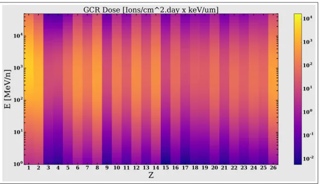
Galactic cosmic radiation originates from outside the solar system and will be incident on astronauts isotropically, i.e. the fluence does not vary according to the direction of measurement. This galactic cosmic radiation consists primarily of ionized particles from Hydrogen (Z=1) to Iron (Z=26) and energies up to 50 GeV/n, shown in Figure 2.2 (Durante and Cucinotta, 2011; Grahn, 1973). While the fluence of ions in space above Z=2 is only 1% of the GCR spectrum, these high Z ions contribute significantly to the radiation dose and dose equivalent.
Figure 2.2: Galactic Cosmic Radiation (GCR) spectrum in free space. The abscissa of the plot is the ion charge Z ranging from proton (Z = 1) to Iron (Z = 26). The ordinate is the energy of the ions in MeV per nucleon. The colors represent the fluence rate of particles.
High Z ions contribute more to the total absorbed radiation dose due to their higher stopping power. Figure 2.3, shows the radiation dose from GCR as a function of energy and ion charge Z. The dose plot of Figure 2.3 was created by multiplying the fluence of particles by their represen-tative stopping power in water. The relative dose contribution from protons, the largest fraction of the GCR fluence, is reduced when converted to absorbed dose. When compared to the fluence plot of Figure 2.2, the dose from higher Z ions, such as oxygen (Z=8) and iron (Z=26), is enhanced.
2.4.3 Radiation protection and quality factors for space
The astronaut occupation is exceptional and risk related to travel from Earth to space is far from negligible. However, it was formally recognized as early as 1969 that the effects of long duration radiation exposure during inter-planetary missions and extended stays at space stations needed to be studied. In 1989, the NCRP published specific recommendations for space activities in Report 98 Guidance on Radiation Received in Space Activities (NCRP, 1989). Career limits for exposure to radiation for astronauts were suggested that would limit the probability of developing
Figure 2.3: Contribution of absorbed dose from Galactic Cosmic Radiation (GCR) spectrum in free space. The abscissa of the plot is the ion charge Z ranging from proton (Z = 1) to Iron (Z = 26). The ordinate is the energy of the ions in MeV per nucleon. The colors represent the contribution to radiation dose. Note, the units for this plot are a surrogate for radiation dose and are not converted to J/kg in tissue.
fatal cancer to an absolute excess risk of 3%. This limit was translated into dose equivalent and based on age and gender for the first time (Table 2.3). Short term limits were also recommended for protection against deterministic (non-stochastic) effects to parts of the body such as the blood forming organs (BFO), lens of the eye and skin and are shown in Table 2.4. However, these limits were meant to be applied to exposures in low earth orbit and not other space situations, such as a mission to Mars (NCRP, 2000).
Table 2.3: Career whole body dose equivalent limits based on a lifetime excess risk of cancer mortality of 3⇥ 10 2
Age (Years) Female (Sv) Male (Sv)
25 1.0 1.5
35 1.75 2.5
45 2.5 3.2
Table 2.4: Short term dose equivalent and career limits for protection against non-stochastic effects (Sv) to the blood forming organs (BFO), lens of the eye and the skin.
Time Period BFO Lens of the Eye Skin
30 day 0.25 1.0 1.5
Annual 0.5 2.0 3.0
Career See Table 2.3 4.0 6.0
The information needed to provide recommendations for missions beyond low-earth orbit was discussed in NCRPs report No. 153 and commentary 23 (NCRP, 2006, 2014). NCRP commentary 23 stated that it is reasonable to use the low earth orbit guidelines of 3% limit on the risk of exposure-induced death (REID), evaluated at the 95% confidence interval of the risk probability distribution function (PDF), as a starting point for future guidelines (NCRP, 2014). However, no specific recommendations were made for radiation protection limits of exploratory missions, due to the large uncertainty in REID and potential cardiovascular and central nervous system (CNS) effects.
Cucinotta et al. introduced revised quality factors based on available radiobiology data and heavy ion track structure based models (Cucinotta et al., 2013). These quality factors take into account more ion track structure and radiobiological information then the LET based ICRP quality factor. The NASA proposed quality factor for space radiation with atomic number Z and velocity
, is given as: QN ASA(Z, ) = (1 P (Z, )) + 6.24 (⌃0/↵ ) LET · P (Z, ), (2.17) where P (Z, ) = ✓ 1 e (Z⇤/ ) 2 ◆m · PT D, (2.18) Z⇤ = Z(1 e 1.25Z2/3· ), (2.19) and PT D= (1 e E ET D). (2.20)
The NASA quality factor also takes into account the different RBE for induction of leukemia and solid cancers using the parameters m, , ⌃0, and ↵ .
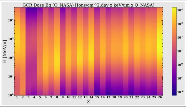
The dose equivalent contribution based on the updated NASA quality factor is shown in Figure 2.4. Implementation of the above NASA quality factor will introduce significant challenges to the development of radiation detectors. These revised quality factors challenge current systems pri-marily due to the complexities of identifying particle charge Z and energy E. While measurement of particles properties are possible on earth, it becomes significantly more challenging under the size, weight, and data bandwidth constraints of space.
Figure 2.4: Contribution of dose equivalent from Galactic Cosmic Radiation (GCR) spectrum in free space. The abscissa of the plot is the ion charge Z ranging from proton (Z = 1) to Iron (Z = 26). The ordinate is the energy of the ions in MeV per nucleon. The colors represents the contribution to radiation dose equivalent. Note, the units for this plot are a surrogate for radiation dose equivalent and are not converted to the unit of Sv.
The challenge of creating a radiation detector compatible with the revised NASA quality factor has motivated several different solutions. One solution, proposed by Borak et al., was to keep all of the features of the NASA quality factor but retain the dependence solely on LET (Borak et al.,
QBorak(LET ) = (1 P (LET )) + ⌃L
LET · P (LET ), (2.21)
where
P (LET ) = (1 e LET⇤ )m. (2.22)
The coefficients ⌃L, ⇤ and m are new model parameters, defined for both leukemias and solid cancers, and selected to closely agree with the NASA quality factors. Another potential solution has been proposed by Pinsky et al. that utilizes a complex radiation detector capable of track imaging to acquire the information necessary for the NASA quality factor (Pinsky and Chancellor, 2007).
2.5 Active radiation detectors
Many active radiation detectors have been used by the United States space program to measure the radiation environment in space (Badhwar, 2004; Hassler et al., 2012; Spence et al., 2010; Zeitlin et al., 2004). Active radiation detectors provide near real time results as opposed to passive detection systems that have to be evaluated at a later time. Additionally, active radiation detectors are capable of providing spatial and temporal information about the environment. A brief review of compact, low power consumption, active radiation detection systems used or proposed for use outside of low-earth orbit follows.
The Martian Radiation Environment Experiment (MARIE) was the first active radiation de-tector specifically designed to measure the radiation exposures astronauts would receive on Mars (Zeitlin et al., 2004). MARIE was one of the three instruments aboard the 2001 Mars Odyssey spacecraft injected into the orbit of Mars in October 2001. MARIE consisted of eight silicon de-tectors of varying thickness; a pair of 1 mm, four 5 mm and a pair of 300 µm. Particles between helium Z = 2 and neon Z = 10 are accurately measured over an energy range of 70 MeV/n to 500 MeV/n (Zeitlin et al., 2003). Additionally, protons are measured in the energy range of 30 to 100 MeV. The detector system had a mass of 3.3 kg and power consumption of 4 W. Particles with
tion of the detector. Algorithms for particle identification based on MARIE data were mentioned but documentation on specific results of the classification effectiveness was not found (Lee et al., 2003).
The Radiation Assessment Detector (RAD) was deployed to Mars as a part of the Mars Science Laboratory (MSL) spacecraft (Hassler et al., 2012). The RAD was mounted on the top deck of the Curiosity rover and took radiation measurements inside the MSL during its 253 day cruise to Mars (Zeitlin et al., 2013). RAD consists on three 300 µm thick silicon detectors as well as scintillators to measure neutrons, not discussed in this work. The RAD detector is very compact with a total volume of 240 cm3 and mass of 1.56 kg. RAD was designed with some basic segmentation that allowed the detector to only measure (accept) ions that traveled a well defined path in the detector. This technology utilized the coincidence and anti-coincidence concepts and also allowed for the measurement of neutrons. RAD was also designed to provide some of the necessary information of the revised quality factors of NASA that require knowledge of the Z and E of the incident particles. RAD was capable of measuring the total energy E for protons up to 100 MeV, carbon ions up to 200 MeV/n, iron ions up to 500 MeV/n and LET of charged particles over the range 0.2 to 1000 keV/µm (Zeitlin et al., 2013).
The Timepix is a position sensitive pixelated detector developed at CERN under the Medipix collaboration (CERN; Llopart et al., 2001, 2007). The Medipix family of detectors, including the Timepix, was developed to meet the needs of the complex Large Hadron Collider experiment. The Timepix detector consists of 256 x 256 55 µm square pixels for a total detection area of 2 cm2 (Pinsky et al., 2011a). Similar to RAD, the sensor layer of the Timepix detector is made of silicon and is 300 µm thick. The unit weighs approximately 20 g and has dimensions of 8.6 x 2.1 x 1.0 cm3. Power for the unit is supplied by a standard USB port on a laptop within the spacecraft or habitat and power requirements are below 2 W (Vykydal and Jakubek, 2011).
An attractive property of the Timepix detector is that radiation tracks of incident particles can be visualized (Hoang et al., 2014; Pinsky et al., 2011a). Initial results have been published doc-umenting the challenges and potential benefits for ion charge and energy discrimination with the
Timepix detector (Pinsky et al., 2011b; Stoffle et al., 2012). However, these results do not clearly state the true positive rate, false positive rate, or other similar metrics for charge classification of heavy ions. Vilalta et al. published on the use of various machine learning techniques for classifi-cation of Si, Fe, O, N and Ne ions of similar LETs and concluded that a predictive accuracy of 81% was possible (Vilalta et al., 2011). However, classification accuracy for individual particles was not presented. Hoang et al. showed that it was possible to determine the angle of incidence and LET for heavy ions based on analysis of track images from the Timepix detector (Hoang et al., 2012, 2014). Additionally, Hoang showed that it was possible to distinguish between protons (Z=1) and helium ions (Z=2) using a variety of machine learning techniques (Hoang, 2013).
Despite all the research in this area, current detector systems and analysis methods have limited capabilities in identification of individual ion charge values (Z). Chapter 6 will present results from the use of a machine learning algorithm to classify ion charge in a space radiation field.
2.6 Conversion of stopping power in silicon to stopping power
in water
Energy deposition in silicon detector systems is not equivalent to energy that would be de-posited in tissue equivalent materials (e.g., water). Biological effectiveness of heavy ions is studied using the concepts of LET in water. Therefore, conversion of energy deposition in silicon to that in water is required for the use of quality factors and relative biological effectiveness. In 1998, Bradley et al. performed Monte Carlo studies to determine the appropriate factor for converting energy deposition in silicon to deposition in tissue and arrived at a factor of 0.63 (Bradley and Rosenfeld, 1998). The study of Bradley et al. was related to boron neutron capture therapy and a specific geometric setup and is not directly applicable to the GCR component of space radiation in this study. In 2008, Guatelli et al. also performed Monte Carlo studies and determined a ratio of 0.56 was appropriate for converting energy deposition in silicon to water (Guatelli et al., 2008). Guatelli et al. specifically focused on the conversion factor for high energy protons with energies
A GCR specific conversion factor was found in two different articles by Zeitlin. In 2010, Zeitlin et al reported that stopping power (dE/dx) in silicon is approximately related to LET in water by the constant 0.56 (Zeitlin et al., 2010). The conversion factor of Zeitlin et al. was reported in measurement data of the MARIE detector and agreed with the results of Guatelli et al. In 2013, Zeitlin et al. again reported a conversion factor in results of the RAD detector measurement on a trip to Mars. In this paper, Zeitlin et al. indicated the average value of the ratio LET in water to dE/dxin silicon is 0.625 for GCRs, with an associated uncertainty of 15% (Zeitlin et al., 2013). This 2013 conversion factor agreed with the results of Bradley et al. Results from this study on the appropriate ratio are presented in Section 5.2.2.
Chapter 3
Radiation transport methods and simulation designs
Modeling the passage of radiation through a medium has numerous applications in space radi-ation and hadron therapy. In space, understanding the impact of radiradi-ation on electronics, habitat materials and crew are important. For hadron therapy, accurate dosimetry is essential for treatment planning and only possible via computational models. Additionally, physical radiation detection systems have limited capability to measure patterns of energy deposition on the nanometer scale and studies at this scale are only possible computationally. The widely used method for computa-tional modeling of radiation transport is the Monte Carlo method.Monte Carlo methods are a statistical technique that have been used extensively to solve prob-lems in areas of math, physics, biology, finance and economics. The modern Monte Carlo method was invented in 1946 by Stanislaw Ulam while he was at Los Alamos National Laboratory working on the nuclear weapons projects (Metropolis, 1987). The dramatic increase in computational power and corresponding decrease in cost have made Monte Carlo methods an important tool. Further-more, Monte Carlo based simulations can provide more geometric flexibility and rapid progress than physical experiments. This work focuses on Monte Carlo methods to simulate complex radi-ation interactions and detector designs.
3.1 Radiation Transport and Monte Carlo methods
The Monte Carlo process can be understood by considering a hypothetical particle that inter-acts via two processes (Kawrakow, 1999). The two processes to consider are: absorption with total cross section aand elastic scattering with total cross section e. The generation of particle trajectories through a medium can then be computed using the following steps:
2. Sample a random distance to the next interaction from a probability distribution function (pdf).
3. Transport the particle to the new interaction coordinate.
4. Select the interaction type based on the probability of absorption, a/( a + e), and the probability of scattering e/( a+ e)
5. Compute or sample the selected interaction.
6. If secondary particles are created at this step they are introduced into the simulation and their trajectories will progress in the same manner.
7. Repeat steps 1 - 4 above until the boundaries of the problem are satisfied.
Radiation transport of real world scenarios are significantly more complex than the hypothet-ical particle presented. Large collaborations of scientists and software engineers have developed programs to handle the complexity of these simulations. Geant4, a toolkit for simulating the pas-sage of particles through matter, is arguably one of the largest and most ambitious Monte Carlo projects (Geant4).
3.2 Geant4 Monte Carlo Toolkit
The Geant4 Monte Carlo toolkit, with its building block design, was chosen for this project (Agostinelli et al., 2003; Allison et al., 2016, 2006). With this software, space radiation detector experiments can be carried out virtually, without the use of expensive ground-based accelerator facilities. New detector designs can be validated virtually before costly construction. These simu-lations are only as good as their design, and each component of the radiation transport simulation and analysis methods must be carefully selected and well defined. In the following sections, the physics models and associated simulation parameters are described.
3.2.1 Physics list selection
In Geant4, the physics models used in the simulation need to be defined before the code can be run. Individual physics models that take into account specific physical interactions are defined and grouped into "lists" to cover a wide range of interactions types and energy ranges. Appropriate selection of the physics models is of great importance for accurate simulations. Based on the work by Ivantchenko et al. the QBBC physics list was chosen for these simulations (Ivantchenko et al., 2012). This physics list includes many different models and seeks high precision in many hadron-ion and ion-ion interactions over a wide energy range.
In Geant4, "energy thresholds" are defined along with the physics list and are used to control the simulations. Simulating every possible particle until they have lost all their energy is compu-tationally impractical and time consuming. Energy thresholds allow the user to quickly modify which particles Geant4 decides to simulate.
Which particles Geant4 simulates, based on the energy threshold defined by the user, can be described in two steps. First, a physical interaction between a particle and its target is simulated and potential secondary particles are stored. Second, the Geant4 code checks the energy thresholds defined before determining which secondary particles are introduced back into the simulation and transported. If the kinetic energy of a particle is less than the threshold energy, it is not created and the energy of that particle is deposited at the location of interaction. The primary particles and higher order particles generated, above the threshold, are transported until they lose all of their energy.
In Geant4, energy thresholds are implemented as range cuts. The range of a potential secondary particle, in the material of interest, is computed. If the range is below the range cut, the particle is not generated and energy is deposited locally. Table 3.1 shows the range cut and energy threshold values used in these simulations. It is important to note that heavy ions range cuts are not included in Table 3.1. Heavy ions have no lower limit of production other than the physical constraints on the interaction and are simulated to zero range after they are produced.
Table 3.1: Geant4 simulation settings: range cuts and energy production thresholds for various particles in water and silicon
Particle Range cut Energy threshold (water) Energy threshold (silicon)
gammma 1 km 10 GeV 10 GeV
e- 1 km 10 GeV 10 GeV
e+ 1 km 10 GeV 10 GeV
proton 700µm 70 keV 70 keV
3.2.2 Computer hardware and data size
All simulations were performed using a high-performance cloud-based Linux cluster available through the Amazon Elastic Compute service. Output data from the simulations were analyzed using custom software written in the Python programming language. Separate computation op-timized and memory opop-timized clusters were used for the Geant4 simulations and data analysis respectively. Monte Carlo output datasets were 2 - 5 Gb in size and dependent on shielding and detector type, with 50 Gb total of simulation data analyzed.
3.3 Simulation design
For this study, three different simulations were created: 1) idealized detector system, 2) real detector system and 3) particle identification system. The similarities between the systems will be discussed first. Section 3.3.1 describes the general geometric setup that all the simulations have in common. Section 3.3.2 describes the incident spectrum of particles used, while Section 3.3.3 provides the general method for recording simulation results including the format of the simulation output data.
The unique features of each system are discussed in the appropriate sections that follow. Sec-tion 3.3.4 discusses the specific geometry of the idealized detector system used to determine appro-priate detector spatial resolution. Section 3.3.5 discusses the specific geometry of the real detector system used to investigate the energy resolution of a detector system. Section 3.3.6 discusses the unique geometric features of the particle identification system.
3.3.1 General geometric setup
The geometric setup was designed to replicate the environmental conditions of a space-based detector system and is represented in Figure 3.1. Spacecraft shielding is often composed of alu-minum due to its strength and low weight. Alualu-minum shielding, of thickness 2 cm, 5 cm and 10 cm, was placed downstream from an ion beam directed at the center of the shield and normal to the surface. The coordinate system of the simulation was defined with the x and y dimensions of the system extending laterally and the positive z direction extending downstream. The origin of the simulation, (x=0, y=0, z=0), is defined as the center of the detector at the back of the shield-ing. Positive z values start at the back of the shielding and extend downstream from the location primary ions are generated.
Figure 3.1: Geometric setup for experiment showing ion normally incident on shielding material with detector downstream. The detector segmentation and size shown are representative and were not used in the final design, discussed later in this paper.