4D PROCESSING AND TIME-LAPSE AZIMUTHAL AMPLITUDE ANALYSIS USING LEGACY SURVEYS FOR NIOBRARA RESERVOIR CHARACTERIZATION,
WATTENBERG FIELD, COLORADO
by
© Copyright by Abdullah Nurhasan, 2017 All Rights Reserved
A thesis submitted to the Faculty and the Board of Trustees of the Colorado School of Mines in partial fulfillment of the requirements for the degree of Doctor of Philosophy (Geophysics). Golden, Colorado Date__________________ Signed: _____________________ Abdullah Nurhasan Signed: _____________________ Dr. Thomas L. Davis University Professor Emeritus Thesis Advisor Golden, Colorado
Date__________________
Signed: _____________________ Dr. John H. Bradford Professor and Head Department of Geophysics
ABSTRACT
Understanding changes in reservoir properties with time due to hydraulic fracture stimulation and production is important. Time-lapse (4D) seismic data analysis enables investigation of stimulated and produced reservoir volumes and helps forecast reservoir performance. Time-lapse seismic has proven beneficial for monitoring conventional high porosity reservoirs but its application to unconventional reservoirs is still in its infancy.
Monitoring unconventional reservoir properties relies on the investigation of the natural fracture network affected by stimulation and production.
This study investigates the potential of legacy seismic surveys for time-lapse azimuthal anisotropy analysis in Wattenberg Field, Denver Basin, Colorado. A workflow for co-processing and methods of analyzing reservoir changes using legacy surveys is developed. The workflow and methods can be used in Wattenberg and potentially in other resource plays. The application of legacy 4D surveys to analyze unconventional reservoirs requires careful applications of cross-equalization for preservation of time-lapse amplitude changes. Despite the differences in
acquisition geometries and parameters this study resulted in normalized root mean square (NRMS) differences of .28 or 28% in the overburden interval above the Niobrara. A widely accepted threshold of .30 or 30% is considered as a measurable index of excellent repeatability.
Azimuthal amplitude variation analysis is used to detect the orientation of the isotropy plane. The azimuth of the isotropy plane indicates the dominant orientation of the fractures affecting seismic anisotropy. Fracture orientation does not always coincide with the maximum horizontal stress. A reduction in amplitude variation with azimuth is observed near faults and is postulated to be a result of multiple fracture orientations. This study provides new insight by illuminating fracture orientations that were not captured by microseismic data or image logs in horizontal wells.
Time-lapse analysis in azimuthal amplitude variation shows anisotropy increases in the reservoir interval. The increase in anisotropy from baseline to monitor is interpreted as being caused by gas coming out of solution in the more fractured parts of the reservoir. Investigating changes in the azimuth and magnitude of anisotropy is beneficial for monitoring unconventional reservoirs.
TABLE OF CONTENT ABSTRACT ... iii LIST OF FIGURES ... vi LIST OF TABLES ... xi ACKNOWLEDGMENTS ... xii CHAPTER 1 INTRODUCTION ... 1 1.1 Research Questions ... 3 1.2 Objectives ... 4 1.3 Scope of Work ... 5 1.4 Thesis Organization ... 5
CHAPTER 2 INTERPRETATION OF WRENCH-FAULTING AND FAULT-RELATED PRESSURE COMPARMENTALIZATION, WATTENBERG FIELD, DENVER BASIN COLORADO ... 7 2.1 Abstract ... 7 2.2 Introduction ... 7 2.3 Structural Interpretation ... 10 2.4 Acoustic Impedance ... 15 2.5 Fault Compartmentalization ... 17
2.6 Prediction of Pressure Difference ... 19
2.7 Incorporating the Effective Stress Coefficient (η) ... 21
2.8 Minor Fault Interpretation from Gamma Ray Logs ... 22
2.9 Mud Log Observation ... 25
2.10 Summary ... 27
CHAPTER 3 PROCESSING OF THE LEGACY SURVEYS ... 28
3.1 Acquisition Parameters ... 28
3.2 Co-Processing Workflow ... 31
3.3 Intermediate Difference Evaluation ... 36
3.4 4D Binning ... 37
3.4.1 Implication of 4D Binning using OVT Mapping ... 40
3.6 Improving Repeatability after Migration ... 42
CHAPTER 4 FORWARD MODELING OF THE AZIMUTHAL VELOCITY AND AMPLITUDE VARIATION ... 48
4.1 Modeling of the Azimuthal Velocity Variation ... 48
4.2 Modeling of the Amplitude Variation with Azimuth ... 56
4.3 Modeling of Time-lapse Change in the Azimuthal Amplitude Variation ... 61
CHAPTER 5 ANALYSIS OF AMPLITUDE VARIATION WITH AZIMUTH ... 65
5.1 Data Quality Control ... 65
5.1.1 Quality Control (QC) of the Offset and Azimuth Distribution ... 65
5.1.2 Rose Diagram Analysis ... 66
5.1.3 QC of the Bandwidth Spectrum ... 68
5.2 Data Pre-conditioning ... 68
5.2.1 Application of Trim Static ... 69
5.2.2 Application of the Bandwidth Matching ... 70
5.2.3 Generation of Common-Offset Common-Azimuth (COCA) Gathers ... 71
5.3 Azimuthal AVO Analysis ... 72
5.4 Azimuthal AVO Volume ... 76
5.4.1 QC of the Anisotropy Map ... 80
5.5 Interpretations ... 81
5.5.1 Interpretation of Anisotropy Gradient Map ... 81
5.5.2 Interpretation of Anisotropy Difference Map ... 85
5.6 Correlation to Production Data ... 87
CHAPTER 6 CONCLUSIONS AND RECOMMENDATION ... 91
6.1 Conclusions ... 91
6.2 Recommendations ... 91
LIST OF FIGURES
Figure 1.1. Timeline of the legacy surveys acquisition and producing section. ... 3 Figure 2.1. A) Stratigraphic Column of Wattenberg Field. B) Geologic Events of Watten-
berg Field. Hydrocarbon reservoirs are marked in green, potential source rocks are marked in purple, and potential coal-bed methane reservoirs are marked in red. (Modified from Higley and Cox, 2007) ... 8 Figure 2.2. Location of the study area. Johnstown (J.), Longmont (Lo.), and Lafayette (La.)
Wrench Faults were interpreted by Weimer (1996) (Modified from Higley and Cox, 2007)... 9 Figure 2.3. A model of rotated blocks by surrounding wrench faults. The 50 square mile
study area is located between the Longmont WFZ and the Lafayette WFZ. ... 10 Figure 2.4. Time structure map of the top of the Niobrara depicts a series of both dextral
and sinistral faults. Warm colors show the highs and the cool colors show the lows. Red arrows show the direction of the fault step-over. Note that the dis- tance of the seismic survey to the Lo. and La. WFZ does not represent the real distance. ... 11 Figure 2.5. Time structure map from the Lower Pierre. The change in fault strike in this
level indicates the rotation of the maximum horizontal stress. ... 12 Figure 2.6. Fault interpretation on the basement level. Fault strike is interpreted using
coherency attributes. ... 13 Figure 2.7. Structural interpretation of the fault episodes in the Wattenberg Field. The
inserted map shows the location of the section. ... 14 Figure 2.8. Vertical impedance model. Green colors represent high impedance. Purple co-
lors represent high impedance. A decrease in impedance is shown from the interval above the Lower Pierre to the top of the Niobrara. Inserted log: p-wave velocity. ... 16 Figure 2.9. Averaged impedance map from the interval representing B chalk, B Marl, C
chalk. The blue dashes represent the stress boundaries. Grey square shows the location of the horizontal wells section. ... 17 Figure 2.10. Well log comparison between well A and well B. Both wells show the same
gamma ray and resistivity trend. The average of velocity difference in the
Niobrara B and C chalk is 6% ... 18 Figure 2.11. The incoherence attributes overlain by the gamma ray log. Orange lines indi-
cate major faults whose presence and orientation can be predicted using incoherence attributes. Blue lines are sub-seismic faults identified in the
Figure 2.12. Average impedance map from the Niobrara interval overlain by the incohe- rence attributes and gamma ray logs. Blue dashes show minor faults whose presence is indicated by the gamma ray logs. The orientation of the minor faults is interpreted from impedance map. Impedance compartmentalization caused by the step-over fault is shown in red arrows. Blue rectangles show
chalk interval that are compared for mud log analysis. ... 24
Figure 2.13. Gamma ray and mud log from well 1, 2, 3, and 4 from right to left. The posi- tion of the panel depicts the relative position of the wells from west to east. Black markers show faults interpreted from gamma ray logs. ... 26
Figure 3.1. Acquisition geometry of the baseline survey using Lockhart Wave. ... 28
Figure 3.2. Acquisition geometry of the monitor survey using a conventional orthogonal set-up. ... 29
Figure 3.3 Offset and azimuth distribution from both surveys ... 29
Figure 3.4. Fold map of the baseline survey. ... 30
Figure 3.5. Fold map of the monitor survey. ... 30
Figure 3.6. Amplitude spectra from both surveys extracted from the shot gather. ... 31
Figure 3.7. Legacy surveys co-processing workflow. Flows 2, 4, and 6 are the common processing workflows, while 1, 3, and 5 are the equalization efforts to bring the monitor closer to the baseline. ... 32
Figure 3.8. Shot gather from the baseline survey after deconvolution. The reflectors are more coherent. The sig- nal is more focused. Noise from ground roll and air blast is still observed. ... 34
Figure 3.9. Shot gather from the monitor survey after deconvolution. The reflectors are more coherent. The sig- nal is more focused. Noise from ground roll and air blast is still observed. ... 34
Figure 3.10. Shot gather from the baseline survey after deconvolution and noise attenuation. The reflectors are more coherent. The signal is more focused. Compared to Figure 3.8, noise from ground roll and air blast has been attenuated. ... 35
Figure 3.11. Shot gather from the monitor survey after deconvolution and noise attenuation. The reflectors are more coherent. The signal is more focused. Compared to Figure 3.9, noise from ground roll and air blast has been attenuated. ... 35
Figure 3.12. A stacked section from the baseline survey. Processing steps from Flow 2 were applied. The stacked section is noisier than the section from the monitor (Figure 3.13). ... 36
Figure 3.13. A stacked section from the monitor survey. Processing steps from Flow 2 were applied. The stacked section has higher signal-to-noise ratio because it has higher fold number than the baseline. ... 37
Figure 3.14. Illustration of OVT Mapping. Only tiles containing traces from both surveys will be included in the PSTM. ... 39
Figure 3.15. Number of fold from both surveys after OVT Mapping and trace number
equalization. ... 39 Figure 3.16. Illustration of the azimuth discrepancy caused by the trace distance. Trace dis-
tance of 600 feet causes 20 degree in azimuth discrepancy to a 3000 feet of offset. The same trace distance causes 11 degree in azimuth discrepancy to 6000 feet of offset. ... 40 Figure 3.17. PSTM results of both baseline and monitor surveys without prior OVT Map-
ping. Although both volumes were migrated using the same velocity, a signifi-cant amplitude discrepancy is observed. NRMS difference between both
volumes is 46% (threshold = 30%). ... 41 Figure 3.18. PSTM result of both baseline and monitor surveys with prior OVT Mapping.
Repeatability is improved. NRMS difference between both volumes is 28% (threshold = 30%). ... 42 Figure 3.19. Left panel: seismic stacked section after trim static. Right panel: NRMS diffe-
rence calculated at each sample. ... 43 Figure 3.20. Amplitude spectrum and phase from both surveys after PSTM and stacking ... 44 Figure 3.21. Amplitude spectrum and phase from both surveys after PSTM, stacking, and
shaping filter applied. ... 45 Figure 3.22. Left panel: seismic stacked section after shaping filter. Right panel: NRMS
difference after shaped filter calculated at each sample. Red polygon shows a chaotic event with high NRMS. ... 46 Figure 3.23. Left panel: seismic stacked section after time variant time shift. Right panel:
NRMS difference after shaped filter and time shift calculated at each sample. NRMS improves significantly for the events with low amplitude. Red polygon shows a chaotic event with high NRMS. ... 47 Figure 4.1. Velocity variation with angle on a VTI medium. The increase in velocity with
angle is because ϵ(1) is positive, which yields a faster velocity in the horizon- tal direction. ... 54 Figure 4.2. Velocity variation with angle and azimuth on a HTI medium. Along the X1
axis (symmetry plane), the velocity decreases with angle. HTI characteristic yields the same velocity between X1 and X3 axis ([X1,X3] becomes the isotro- py plane). ... 55 Figure 4.3. Velocity variation with angle and azimuth in an orthorhombic medium. Velo-
city variation depends on the ratio between the stiffness or the compliance ten-sors (caused by the fractures) on the [X1,X3] and [X2,X3] plane. ... 56 Figure 4.4. Reflectivity variation with angle and azimuth. Reflectivity represents the
boundary between isotropic/HTI media. The elastic properties and anisotropy parameters are listed in Table 4.1. ... 60 Figure 4.5. Changes in reflectivity variation with angle and azimuth. Reflectivity repre-
the reflectivity of the baseline survey, and dashed lines represent the reflecti- vity of the monitor survey. The elastic properties and anisotropy parameters are listed in Table 4.2. The model shows that the AVO gradient on the non-zero azimuth increases with the increase in HTI magnitude. ... 63 Figure 5.1. Example of the offset and azimuth distribution of baseline and monitor survey
from 1 CDP bin. Red star shows the location of the center of the CDP bin. Black dots show the location of the trace that represents the offset and azimuth relative to the center of the CDP bin. ... 66 Figure 5.2. Iterations of the rose diagram analysis. A) Azimuth bins are centered at 0
(north) and 90 (east). B) Azimuth bin centers are shifted by 5 degrees. ... 67 Figure 5.3. Wavelet and average amplitude spectrum of both surveys before bandwidth
equalization. Blue curves are from the baseline and green curves are from the monitor. The spike at 8Hz is one of the targets for equalization. ... 69 Figure 5.4. Gathers A) without and B) with trim statics and time-shift correction. Trim
sta-tics flatten the gather to enable amplitude investigation along the offset and
azimuth. ... 70 Figure 5.5. Wavelet and average amplitude spectrum of both surveys after bandwidth
equalization. Blue curves are from the baseline and green curves are from the monitor. The low and high frequency ranges are now equalized. ... 71 Figure 5.6. COCA gather for azimuthal AVO analysis. Trim statics have been applied to
flatten the events. The red rectangle shows that the near offset that lacks distribution of traces in the azimuth bins. The green rectangle shows the far offset with better trace distribution throughout the azimuth bins. ... 72 Figure 5.7. Azimuthal AVO analysis at location 1 (the middle of Gobbler East). Different
colored curves repre-sent different incidence angles. Despite differences in
amplitudes, both surveys exhibit same anisotropy gradients. ... 73 Figure 5.8. Azimuthal AVO analysis at location 2, near the producing wells of Gobbler
East. Different colored curves show different incidence angles. Difference in anisotropy gradients is observed, indicating increase in anisotropy from base- line to monitor. ... 74 Figure 5.9. Azimuthal AVO analysis at location 3, the middle of Gobbler West. Different
colored curves show different incidence angles. As in Figure 5.8, difference in anisotropy gradients is observed, indica- ting increase in anisotropy from
baseline to monitor. ... 75 Figure 5.10. Summary of the time-lapse azimuthal amplitude variation analysis of three
different locations. Loca-tion 2 falls under case 2 and location 3 falls under case 1. ... 76 Figure 5.11. Anisotropy gradient of the top of the Niobrara Formation extracted from the
baseline survey. Orange color shows high anisotropy, white color shows low anisotropy. ... 78
Figure 5.12. Anisotropy gradient of the top of Niobrara Formation extracted from the moni- tor survey. Orange color shows high anisotropy, white color shows low
anisotropy. ... 78 Figure 5.13. Orientation of the azimuth of the isotropy plane in each CDP from the baseline
extracted from the top of the Niobrara Formation. The dashed line shows the edge of the survey. ... 79 Figure 5.14. Orientation of the azimuth of the isotropy plane in each CDP from the monitor
extracted from the top of the Niobrara Formation. The dashed line shows the edge of the survey. ... 79 Figure 5.15. Difference in anisotropy gradient of the top of Niobrara Formation. Yellow
color shows high increase (positive change), orange color shows high decrease (negative change). The dashed line shows the edge of the survey. ... 80 Figure 5.16. Azimuthal velocity model for an orthorhombic medium involving 2 sets of
vertical fractures orthogonal to each other. ... 83 Figure 5.17. Variation of fracture orientation from discrete fracture network. Compared to
the isotropic plane azimuth in Figure 5.13 and Figure 5.14, the azimuth of the fracture orientation can be correlated to the interpretation of isotropic plane
orientation. Modified from Grechishnikova (2017). ... 85 Figure 5.18. Anisotropy differences map compared to the total oil and gas production from
wells in Gobbler West. The total production is calculated per monitor survey acquisition (June, 2013). Well 3 as the highest gas producer exhibits a sharp increase in anisotropy. ... 88 Figure 5.19. Anisotropy differences map compared to the total oil and gas production from
wells in Gobbler West. The total production is calculated per April 2017. The trend from Figure 5.18 continued 4 years after the monitor acquisition. ... 89
LIST OF TABLES
Table 2.1. Percentage Difference in Pressure by the Change of η. ... 22 Table 4.1. Elastic properties and anisotropy parameters of the media used to model for
reflectivity variation with angle and azimuth. ... 60 Table 4.2. Elastic properties and anisotropy parameters of the media used for reflectivity
variation with angle and azimuth. The parameters represent the magnitude of the anisotropy investigated by the baseline and monitor surveys. ... 61
ACKNOWLEDGMENTS
All praise be to Allah, the God of the universe, the all mighty, all knowing, all wise, all bless and merciful.
I would like to thank my advisor Dr. Thomas L. Davis who has, during his last years of advisory, been very passionate to teach how to be a better researcher, and show me how to be an excellent educator as well as an entrepreneur. I thank my thesis committees: Dr. Ali Tura, Dr. Jim Simmons, Dr. Steve Sonnenberg, Dr. Manika Prasad, Dr. Terry Young, and Dr. Bob Benson for their support and belief in me.
I thank Pertamina who has funded my doctorate education at Colorado School of Mines. I thank Anadarko Petroleum Corporation for providing the data set. I thank Reservoir
Characterization Project for providing research facility. I thank people at FairfieldNodal Denver: Kevin Wright, Chuck Czarnecki, Bruce Karr, and Robb Windels for their guidance throughout the 4D processing. I thank the Department of Geophysics, professors in Colorado School of Mines, and all my teachers who have been God’s messengers for delivering the knowledge to me.
I thank my fellow brothers: Dr. Fadli Rahman, Dr. Mohamad Kemal, Dr. Imam Akimaya, and soon to be Dr. Noor Cahyo for our crazy, fun, and inspiring moments of snowboarding, FIFA-ing, biking, traveling, coffees, and all togetherness, loves, and supports you and your family showed me and mine. I thank the family of Pengajian Indonesia in Colorado for being brothers and sisters in iman, for helping me and my family stay true is Islam.
I thank my parents, who has been my biggest support in everything, and my biggest source of love and prayers. I thank my sisters, my father, mother, brothers and sisters in law, and all my family.
And last and most, I thank my beloved wife for sharing this journey and adventure. For being beside me at every moment. For all the love, pray, and support.
CHAPTER 1 INTRODUCTION
Wattenberg Field is the fourth largest oil field in the USA with original oil in place (OOIP) of 4-billion-barrel oil equivalent (BBOE) (Sonnenberg, 2013). The field is located in the Denver Basin. Of interest is the Late Cretaceous Niobrara Formation, which consists of
interbedded chalks and marls (Higley and Cox, 2007; Sonnenberg, 2012). The Niobrara
Formation is an unconventional reservoir in Wattenberg Field with high organic content (as high as 5.8 weight percent). Other than the Niobrara, the production also comes from the Codell sandstone. At early stage (1980’s), the field development was challenged by the low
permeability, making it hard to reach economic production from vertical wells. Early fracture characterization on the Niobrara reservoir is provided by Lu (1988) who analyzed different amplitude versus offset (AVO) response between fractured and non-fractures zones in Silo field Wyoming. The productivity and recovery factor from the Niobrara Formation have increased dramatically through intensified horizontal drilling and multi-stage hydraulic fracturing. Parts of the field are operated by Anadarko Petroleum Corporation (APC), who has provided the
Reservoir Characterization Project (RCP) several seismic surveys for regional structural interpretation and time-lapse analysis.
Monitoring rock property changes within a reservoir is important in both conventional and unconventional reservoir characterization. Studies on time-lapse impedance analysis using P-wave post-stack data have been published (White, 2015; Utley, 2017). Monitoring the elastic properties of the reservoir may potentially illuminate the area of produced reservoir area. In an unconventional reservoir such as the Niobrara/Codell Formations, fractured rocks (naturally and stimulated) contribute most of the hydrocarbon production in the early phase of production. Changes in the reservoir properties are expected due to hydraulic fracturing and production. Hydraulic fracturing aims to enhance permeability by increasing fracture apertures and creating complex fracturing. Increased fracture aperture is expected to change reservoir elastic properties due to the increase in rock compliance. During production, permeable fractured areas will change upon pore pressure depletion (Ning, 2017). Furthermore, fluid alteration inside the
reservoir might be another cause for changes in reservoir elastic properties. Seismic velocity analysis and impedance inversion can be used for detecting these changes. Furthermore, directions/orientations of the fractures affected by the stimulation and production might be different. Motamedi’s study (2015) shows shear wave splitting and anisotropy changes between baseline and monitor surveys. Different changes in fracture compliance may cause an increase or decrease in azimuthal velocity anisotropy. Therefore, this study is not intended to use wide azimuth pre-stack data to enable investigating variation and changes in velocity and amplitude with offset and azimuth for fracture characterization.
Time-lapse/4D seismic survey acquisition, processing and interpretation are integral parts of reservoir monitoring and management. Knowledge of the stimulated and produced reservoir volume may enable enhancing the hydrocarbon recovery factor through optimizing well placement and completions. The reliability of time-lapse seismic depends on survey
repeatability, a parameter dependent on how identical the geometry and parameters are used in baseline and monitor surveys. Efforts in ensuring survey repeatability include planting
permanent geophones for multiple time-lapse surveys. However, in the current economic climate, when cost reduction is paramount, there is a growing need to utilize time-lapse co-processed legacy surveys, which enable companies to conduct 4D seismic investigation at a reduced cost. The term “Legacy Surveys” refers to two or more seismic surveys acquired in the same location (i.e. observing the same target) but with different parameters and/or geometry. The motivation in using legacy surveys for 4D analysis is to utilize existing data to enable time-lapse analysis to evaluate reservoir performance and further benefit economic and business decisions. Time-lapse investigations using legacy surveys become more valuable when the baseline survey was acquired before any stimulation and production has begun. It is impossible to go back in time to acquire the pre-stimulation (or production) to capture the original reservoir condition. In a joint effort between the RCP and FairfieldNodal, I processed two legacy P-wave seismic surveys acquired for APC in Wattenberg Field, Denver Basin Colorado, USA. The baseline survey was acquired in 2010 and the monitor was acquired in 2013.
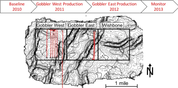
My research goal is to use the time-lapse seismic analysis to characterize anisotropy changes in the reservoir after one year of production in the Niobrara/Codell Formations. The producing sections (Gobbler West and East) are shown in Figure 1.1. The surrounding sections were produced since 2013 (after the monitor survey was shot). I expect to detect the change
within Gobbler West and East and compare that to the other sections. To do this, I compare the velocity, impedance, amplitude variation with angle and azimuth, and frequency between the baseline and monitor. The baseline is the Aristocrat survey shot in 2010. Another survey called Anatoli serves as the monitor, acquired in 2013. To detect changes between these two surveys, an integrated analysis and investigation of the structure in the study area, seismic acquisition and processing, and anisotropy modeling have to be conducted. In this thesis, I document the
structural interpretation, co-processing methodology, anisotropy modeling, and time-lapse anisotropy interpretation for the produced unconventional reservoir. I expect this manuscript can serve as a manual for the industry and researchers who wish to benefit from analyzing time-lapse effect using legacy surveys.
Figure 1.1. Timeline of the legacy surveys acquisition and producing section.
1.1 Research Questions
This thesis will test several hypotheses and answer associated research questions: 1. Co-processing legacy surveys requires meticulous work. The surveys have to be
repeatable for the interpretation to be meaningful. Sub-optimum processing will either leave too much noise on both surveys or over-equalize them so the changes will not be detected. Therefore, the research question I will answer is what processing steps are the most significant for improving repeatability?
1 mile
Gobbler West Gobbler East Wishbone
Monitor 2013 Gobbler East Production 2012 Gobbler West Production 2011 Baseline 2010 1 mile
Gobbler West Gobbler East Wishbone
1 mile
2. Reservoir pressure will decrease with production. However, the reservoir has been hydraulically stimulated. Cracking the rock is not an elastically reversible process. Therefore, the research question is: with the decrease in reservoir pressure during
production, what changes will I see in velocity and impedance within the producing area?
3. Faults and fractures may act as potential fluid conduits or barriers during production. Can I expect to see lateral velocity and impedance variation around the faults that can help us assess the role of faults and fractures in this reservoir?
4. A vertical fracture network might cause a horizontal traverse isotropic (HTI) characteristic. Can I detect the change in velocity and impedance by analyzing the amplitude variation with azimuth?
Characterizing time-lapse changes from a stiff rock such as the Niobrara can be
challenging since the rock property variation is subtle. In this research, I will implement careful processing steps to attenuate the noises from acquisition footprint and previous processing steps. Any attributes will be examined and correlated to ensure that they represent physical meaning of the reservoir time-lapse changes.
1.2 Objectives
The objectives of the study are:
1. To improve the repeatability of the legacy surveys. The improvement is necessary to enable useful interpretation of changes observed between surveys. Improvement is done by applying a same processing work flow as well as equalization of bandwidth,
amplitude, number of traces, and traces distances.
2. To map the time-lapse variation of the velocity and amplitude variation with angle and azimuth. Mapping the changes in the reservoir elastic properties after stimulation and production requires the analysis of pre-stack seismic data.
3. To interpret the produced reservoir volume, and determine the role of the faults and fractures in production. Complex faults network might cause either flow barriers or enhanced connectivity. Therefore, time-lapse analysis will enable interpretation of the role that faults and fractures play in production.
1.3 Scope of Work
The scope of work includes: 1. Structural interpretation within the study area, 2. 4D processing of the legacy seismic data from raw data (shot record) in targeting 4D equalization for time-lapse analysis, 3. Velocity and amplitude anisotropy modeling, 4. Analysis of velocity and amplitude variation with azimuth in static and dynamic conditions.
Several sets of seismic surveys were used in this study. The structural interpretation in Chapter 2 used the regional merged seismic survey that covers a 50 square-mile area. However, the impedance analysis in Chapter 2 uses a smaller area due to data quality (frequency content and fold). This seismic survey covers a 10 square-mile area, which in the time-lapse analysis, acts as baseline survey. The monitor survey also covers roughly the same 10 square-mile area with several differences in geometry and parameters.
1.4 Thesis Organization
This thesis is organized to tackle the aforementioned objectives in order. Chapter 2 discusses the episodes of faulting that have taken place in the study area and investigates how the faulting results in reservoir compartmentalization. The reservoir compartmentalization is
indicated by the lateral variation of P-wave impedance. Then, I discuss the methodology,
workflow, and result of co-processing the legacy surveys in Chapter 3. This chapter discusses the comparison of the survey geometries and parameters, and how the discrepancies can affect the 4D analysis. Chapter 3 presents results of the equalized 4D legacy surveys.
In Chapter 4, I present models of anisotropy using azimuthal velocity and amplitude equations and analysis. I discuss several combinations of fractures orientations and their effects to the azimuthal velocity and amplitude anisotropy. This chapter is a bridge for readers in
Chapters 5 includes anisotropy and 4D analyses based on the structural interpretation from Chapter 2 and anisotropy modeling from Chapter 4.
CHAPTER 2
INTERPRETATION OF WRENCH FAULTING AND FAULT-RELATED PRESSURE COMPARTMENTALIZATION, WATTENBERG FIELD,
DENVER BASIN COLORADO
2.1 Abstract
A structural interpretation of a 50-square-mile 3D seismic data set from Wattenberg Field, Colorado indicates a northeast-trending step-over fault system in the Niobrara Formation. These step-over faults are the product of a fault block rotation that is caused by two large scale dextral wrench faults: the Longmont and Lafayette wrench fault zones. An investigation into different fault orientations between the Niobrara and the overlying Pierre Shale indicates that a rotation of the maximum horizontal stress has occurred during the Laramide Orogeny.
The step-over faults and stress rotation result in reservoir compartmentalization in the Niobrara. Seismic inversion shows the stress field compartmentalization. Low impedance occurs in a lower effective stress environment caused by high pore pressure. These low impedance compartments may constitute “sweet spots” in exploration and production in the Niobrara Formation.
2.2 Introduction
The Niobrara Formation is a major hydrocarbon reservoir deposited during the Late Cretaceous (Figure 2.1.A). This formation consists of the Smoky Hill Member and Fort Hays Limestone. The Smoky Hill member of the Niobrara within the study area consists of B and C chalks, and A, B, and C marls. The chalks are defined as lithology containing more than 70% carbonate, while marls are defined as lithology having 50-70% carbonate content. The Niobrara is a self-sourcing reservoir that is generally overpressured (Sonnenberg, 2012). The overpressure is a result of volumetric expansion caused by hydrocarbon maturation. Bratton (2015) indicates that the overpressure regime extends into the overlying Sharon Springs Member of the Lower Pierre Formation. Figure 2.1.B shows the geologic events of the Late Cretaceous Petroleum
System (Higley and Cox, 2007). One of the important events is the Laramide Orogeny that occurred during the Late Cretaceous and early Tertiary (between 70-50 ma.). This event is thought to be responsible for the recurrent movement of faults in the study area (Higley and Cox, 2007). The products of this movement include several wrench fault zones located in the area mapped by Weimer (1996).
Figure 2.1. A) Stratigraphic Column of Wattenberg Field. B) Geologic Events of Wattenberg Field. Hydrocarbon reservoirs are marked in green, potential source rocks are marked in purple, and potential coal-bed methane reservoirs are marked in red. (Modified from Higley and Cox, 2007)
Weimer (1996) interpreted the northeast-trending wrench faults in Wattenberg Field: the Johnstown Wrench Fault Zones (WFZ), the Longmont WFZ, and the Lafayette WFZ
(Figure 2.2). Higley et al. (2003) correlated of 4000 wells to map the fault system in the Codell Sandstone, a formation underlying the Niobrara. Davis (1985) interpreted the wrench fault
Wattenberg Field Stratigraphic Column
Modified from Higley and Cox 2007 A
system associated with the basement fault block movement using 2D seismic data. His study depicts listric faults in the Niobrara-Carlile and Pierre Formations as the result of recurrent basement movement. The Rocky Mountain Arsenal (RMA) fault recent movement served as evidence of the high stress existence in the basement. The RMA fault is a northwest-trending basement fault whose movement was triggered by fluid injection into the fault zone (Dart, 1985; Evans, 1966).
Figure 2.2. Location of the study area. Johnstown (J.), Longmont (Lo.), and Lafayette (La.) Wrench Faults were interpreted by Weimer (1996) (Modified from Higley and Cox, 2007)
This study investigates the influence of the regional wrench faulting on the reservoir compartmentalization, and indicates that variation in impedance between compartments suggests stress anomalies. Impedance mapping helps to reveal the different stresses distributed throughout the area. This stress mapping is important in helping to target the “sweet spots” in exploration and production. Seismically resolved faults are picked from structural interpretation and
The investigation shows the existence of the minor faults confirming the boundaries interpreted from the impedance map.
2.3 Structural Interpretation
The study area is located between two large-scale dextral strike-slip faults: the Longmont (Lo.) WFZ to the north and the Lafayette (La.) WFZ to the south (Figure 2.2). These northeast-oriented fault zones are associated with faulting from the aforementioned Laramide Orogeny, which occurred at the end of the Cretaceous era and extended into the Early Tertiary (Higley and Cox, 2007). The nature of these two dextral wrench faults results in a sinistral force forming in between the major faults. Figure 2.3 shows a model of an anti-clockwise block rotation resulting from this sinistral force. Two types of strike-slip faults are expected to occur due to this rotation. A sinistral strike-slip will occur in the east side of the block, and a dextral strike-slip will occur in the west. The product of strike-slip faulting is en-echelon faults that are separated by offset called step-over faults (shown by red blocks). Right-stepping faults are observed in a dextral strike-slip and left-stepping fault series are observed in a sinistral strike-slip. These two types of step-over faults are found in the study area at the Niobrara level and confirm the rotation model resulting from the wrench faulting.
Figure 2.3. A model of rotated blocks by surrounding wrench faults. The 50 square mile study area is located between the Longmont WFZ and the Lafayette WFZ.
Longmont Wrench Fault Zone
Lafayette Wrench Fault Zone
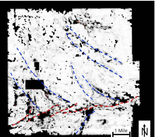
Figure 2.4. shows the time structure map of the top of the Niobrara horizon overlain by an incoherence attribute extracted by White (2015) from the same horizon. The structure map depicts a regional northeast-striking fault series as the result of the larger-scale wrench fault regime. This type of faulting dominates the system at the Niobrara level, creating
compartmentalized grabens denoted by blue-purple colors in Figure 2.4. The throw of these
Figure 2.4. Time structure map of the top of the Niobrara depicts a series of both dextral and sinistral faults. Warm colors show the highs and the cool colors show the lows. Red arrows show the direction of the fault step-over. Note that the distance of the seismic survey to the Lo. and La. WFZ does not represent the real distance.
N
Lo. WFZ
La. WFZ
Well A
faults ranges from 30-130 feet (ft) at the top of the Niobrara. The width of the grabens on the top of the Niobrara varies from 1000 to 1500 ft. A small aspect ratio of the fault block (the ratio between the width to the length of the fault block) indicates that the ratio of the maximum to minimum horizontal stress is greater than one (Cartwright, 1996). A rotation of maximum
horizontal stress can be observed from the change in fault strike in the Lower Pierre (Figure 2.5), a horizon approximately 200 millisecond (ms) above the Niobrara. At this level, the dominant fault strike is northwest-southeast. It can also be observed that the west-striking faults are more prominent at this level, compared to the west-striking faults at the Niobrara.
Figure 2.5. Time structure map from the Lower Pierre. The change in fault strike in this level indicates the rotation of the maximum horizontal stress.
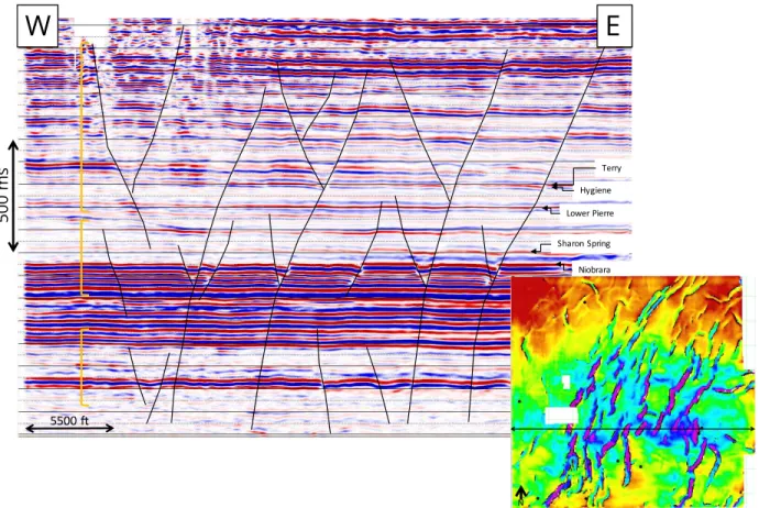
A fault interpretation of the vertical seismic section shows that several main faults have developed from recurrent movement in the basement faults (Figure 2.7). These wrench faults extend from the basement to the Upper Pierre and presumably higher. The strike-slip movement of the basement resulting from the block rotation is shown in Figure 2.6. Coherency attribute was
10000 ft N Well A Well B 20 ms
used for the interpretation of the basement fault strike. The throw of the strike-slip fault may be difficult to resolve (Davis, 1985) as the vertical displacement is commonly less than 20 ft (Higley et al., 2003). Seismic velocity increases with depth causing the Fresnel zone to be larger decreasing the lateral resolution at depth. These strike-slip faults triggered the second episode of
Figure 2.6. Fault interpretation on the basement level. Fault strike is interpreted using coherency attributes.
the fault development; the formation of negative flower structures at the Niobrara and Sharon Springs level (Figure 2.4). Because of the nature of these flower structures, the grabens generated between the fault and the antithetic faults in the Sharon Springs level are large compared to the grabens in the Niobrara. As the rotation of the basement continued toward the end of the Laramide Orogeny, another set of negative flower structures developed in the Pierre Formation, which resulted in the fault orientation seen in Figure 2.5. The sequence of the fault episodes follows the episodes described by Davis (1985). In his work however, due to the
N
limitation of the 2D data, the relation between each episode is not clearly depicted. The 3D seismic data in this study helps to investigate the development of the flower structure in more detail, demonstrating that the basement-level faulting is connected throughout the Upper Pierre by several major wrench faults.
Figure 2.7. Structural interpretation of the fault episodes in the Wattenberg Field. The inserted map shows the location of the section.
Earthquakes near the study area have been recorded as recently as 2014. Five earthquakes with magnitudes of 1.7 to 3.4 and hypocenters between 4-7km were reported near the town of Greeley 12 miles to the north of this seismic survey (earthquaketrack.com). These earthquakes show that a high basement stress regime still exists. Between 1962-1965, 710 waste injection-related earthquakes caused by movement along the RMA fault were recorded (Evans, 1966). The RMA Fault is orienting N45W and extends for 16km (Dart, 1985). Movement of the northwest-orienting RMA fault indicates that the current stress in the subsurface is high. Using the analyses
West East Lower Pierre Sharon Spring Niobrara Codell Terry Hygiene West East 5500 ft
W
E
500 ms 8000 ft Nof borehole breakouts, Dart (1985) and Allen (2010) also indicate that the current maximum horizontal stress is trending northwest.
2.4 Acoustic Impedance
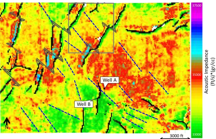
A seismic impedance volume was used to capture the vertical impedance change from the Terry and Hygiene Sandstone in the Upper Pierre to the Carlile Formation. Figure 2.8 shows the impedance section from the crossline near well A and B with sonic logs inserted into the section. The presence of high quartz content (in Terry and Hygiene) is indicated by the high impedance. A trend of decreasing acoustic impedance starts from around 100 ms below Terry and Hygiene sandstone. The general decease in impedance in the Lower Pierre is due to the decrease in velocity caused by overpressure. The increase in pore pressure caused by hydrocarbon maturation decreases the effective stress. Since P-wave velocity is sensitive to stress, the decrease in effective stress will result in the decrease in velocity. The trend of decreasing impedance indicates that overpressure in the Niobrara has extended into the Lower Pierre (Bratton, 2015).
An impedance map was generated in order to study the lateral distribution of the impedance in the chalks interval of the Niobrara (Figure 2.9). The impedance map shows high impedance in the northeast-trending grabens. This high impedance indicates that higher effective stress applies to the grabens. When the grabens were created, a local northwest-trending
extensional regime from the strike-slip movement was applied, causing the grabens to open (relaxation). Due to the northwest orientation of today’s maximum stress regime, the grabens are more compressed than the surrounding area resulting in a higher effective stress and thus higher impedance. It can also be observed that the step-overs can compartmentalize impedance between the grabens.
It is also important to investigate how the impedance model could benefit in mapping the sub-seismic faults. The impedance map shows that at well B, the impedance is lower than at well A, which is located 1500 ft to the northeast. This difference shows that an impedance boundary exists between both wells. This boundary, denoted in blue dashes, suggests sub-seismic faults that act as stress barriers between both wells. The boundary is not only found between wells A and B but also in several other areas. These boundaries, trending mostly northwest, indicate
fault-bound stress compartmentalization that is parallel with the current maximum stress orientation.
The impedance map shows high impedance in the northeast-trending grabens. This high impedance indicates that higher effective stress applies to the grabens. When the grabens were created, a local northwest-trending extensional regime from the strike-slip movement was applied, causing the grabens to open (relaxation). Due to the northwest rotation of today’s maximum stress regime, the grabens are compressed more than the surrounding area resulting in a higher effective stress and thus higher impedance. It can also be observed that the step-overs can compartmentalize the Niobrara reservoir.
Figure 2.8. Vertical impedance model. Green colors represent high impedance. Purple colors represent high impedance. A decrease in impedance is shown from the interval above the Lower Pierre to the top of the Niobrara. Inserted log: p-wave velocity.
While the boundaries of the major grabens and faults are seismically resolved, it is also important to investigate how the impedance model could benefit in mapping the sub-seismic faults. The impedance map shows that at well B, the impedance is lower than at well A, which is
100 ms 3000 ft 37000 25000 30000 Lower Pierre Sharon Spring Niobrara Terry Hygiene Well A Well B Codell Ac o u st ic I m p e d a n ce (ft /s )* (g r/c c)
located 1500 feet to the northeast. This difference shows that an impedance boundary exists between both wells. This boundary, denoted in blue dashes, suggests sub-seismic faults that act as stress barriers between both wells. The boundary is not only found between wells A and B but also in several other areas. These boundaries, trending mostly northwest, indicate fault-bound stress compartmentalization that is parallel with the current maximum stress orientation.
Figure 2.9. Averaged impedance map from the interval representing B chalk, B Marl, C chalk. The blue dashes represent the stress boundaries. Grey square shows the location of the horizontal wells section.
2.5 Fault Compartmentalization
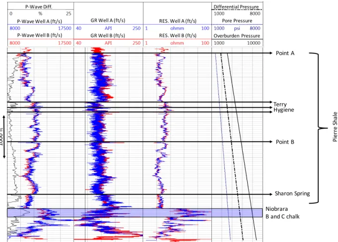
This analysis starts by investigating the vertical velocity trend of two wells A and B. In Figure 2.10, well logs from well A and B are superimposed on each other. In general, the gamma ray trend within the Pierre Formation is constant. This trend suggests minimal lithology change in the Pierre Formation. An exception is found in the Terry and Hygiene Sandstones, where a decrease in gamma ray appears. An increase in quartz content within the sandstones results in an increase in velocity. In the far-left panel, an increase in velocity from depth point A to depth
3000 ft N 37500 35000 33000 Well A Well B Ac o u st ic I m p e d a n ce (ft /s )* (g r/c c)
point B is observed. In a normal stress regime, overburden pressure increases in a higher rate than the pore pressure causing the effective pressure to increase with depth. With minimal lithology variation, a positive velocity trend indicates rock compaction due to the increase in effective pressure. The normal increasing rate of the overburden, pore, and effective pressure is shown in the far-right panel in Figure 2.10. The effective pressure was calculated under the assumption that effective pressure is equal to differential pressure. In spite of a continuing uniform gamma ray trend, a negative trend of velocity is observed from depth point B and continues at depth. This trend is due to the decrease in effective pressure as a result of the
increasing pore pressure. As p-wave velocity depends on stress, observing the velocity trend with depth is useful for investigating the overpressure regime in vertical direction.
Figure 2.10. Well log comparison between well A and well B. Both wells show the same gamma ray and resistivity trend. The average of velocity difference in the Niobrara B and C chalk is 6%
Laterally, the idea of the pressure effect on velocity in a uniform lithology can be used for comparing the velocity between two neighboring wells. The intervals compared are from the
GR Well A (ft/s) GR Well B (ft/s) RES. Well A (ft/s) RES. Well B (ft/s) P-Wave Well A (ft/s) Niobrara B and C chalk P-Wave Well B (ft/s) P-Wave Diff. Differential Pressure Pore Pressure Overburden Pressure Point A Point B Terry Hygiene Sharon Spring 1000 ft Pi e rr e S h a le
B to C chalk in the Niobrara. This step is done to investigate the cause of the difference in impedance shown in Figure 2.9. A difference in velocity between wells A and B in this interval could explain the difference between the impedance between both wells. The average velocity difference in the investigated interval is 6%. This difference can be caused by lithology, porosity, fluid saturation, and pressure changes. The difference in lithology can be identified by the
difference in gamma ray logs while both fluid saturation and porosity might affect the resistivity. Gamma ray and resistivity from both wells are observed to be aligned, eliminating the first three possibilities and leaving the difference in effective pressure as the main reason for impedance change.
2.6 Prediction of Pressure Difference
The difference in pressure between 2 wells was predicted using Eaton’s equation, which states that the ratio of the differential pressure is equal to the ratio of p-velocity to the power of Eaton constant. Eaton (1975) lays out the relationship between pressure and velocity as:
�' �'( = �+ �+( , -(2.1)
where �' is the actual or measured p-wave velocity, �'( is the p-wave velocity in normal pressure, �+ is the actual or in situ differential pressure, �+( is the normal differential pressure, and E is the Eaton constant that depicts the behavior of the rock with pressure. In some cases, differential pressure is equal to the effective pressure. Biot and Willis (1957) formulates the effective pressure as:
�. = �/ − ��' (2.2)
where �. is the effective pressure, �/ the confining pressure, �' is the pore pressure, and � is the
differential pressure (�+), which is the difference between the confining pressure and the pore
pressure. Eaton’s equation indicates that the ratio of two velocities in two different pressures depends on the ratio of the pressure itself. Therefore, to determine E, equation (2.1) can be rewritten as: �'2 �', = �+2 �+, , -(2.3)
where �', is the velocity of the rock in an applied differential pressure �+, and �'2 is the
velocity in �+2. The differential pressure is calculated by subtracting the vertical overburden
pressure with the normal pore pressure trend (0.45 psi/ft). The overburden pressure �345 is the result of the integration of the density of the rock �7 with the depth multiplied by the gravity (equation. 4).
�345 = � �7 9:;4< 9:=
� �� (2.4)
The trend pf the overburden, pore, and differential pressure are displayed in the far right panel in Figure 2.10. Two depth points are taken to calculate E. These two points represent the beginning and the end of the normal pressure regime shown in Figure 2.10. The first velocity and differential pressure are taken from depth point A with 10000ft/s and 2246 psi. The second velocity and differential pressure were taken from point B with 12470 ft/s and 3890 psi. These two points represent the interval of the normal pressure gradient, where the velocity gradually increases with the compaction due to the overburden pressure. Using equation (2.3), E is now equal to 2.4882.
On average, in the B and C chalk interval, the velocity in well A is 6% higher than well B. Using Eaton’s equation, with the calculated E, the ratio between two differential pressures �'+ = (�+2 �+,) is rewritten as:
�'+ = 4AB
4AC
(2.5)
With the actual differential pressure being unknown the ratio of the differential pressure between two well location can be predicted. Using equation (2.5), well A is shown to have 15% more differential pressure than well B.
2.7 Incorporating the Effective Stress Coefficient (�)
Hofmann et al. (2005) suggest that any change in pore pressure needs to be scaled by the effective pressure coefficient (�). They postulate that for rocks with low porosity, � will be significantly lower than 1 and closer to zero. Nur et. al. (1995) suggest that � can be obtained by:
� = �
�/F (2.6)
where �/F is the critical porosity (0.4) for clastic rock. This equation suggests that � will
decrease with the decrease of porosity. The implication of � being lower than 1 is that Eaton’s constant (E) will vary. In predicting E, the pressure applied to the rocks is no longer the differential pressure but rather the effective pressure. Therefore, the notation of the effective pressure (�.) refers back to equation (2.2). The difference in effective pressure can be obtained using: �/2− �2�'2 �/,− �,�', = �'2 �', -H (2.7)
where �J denotes modified Eaton’s constant. To calculate the effective pressure at different
depths, three different values of � were assumed (1, 0.7, and 0.5). �1 is set for the shallower depth, and �2 is set for the deeper level. Due to the compaction of the rock, which results in lower porosity, �2 will be lower than �1. The result shows that applying a different � will result
in Eaton’s constant greater than the original Eaton’s constant calculated using the ratio of the differential pressure. The implication of greater Eaton constant is greater percentage differences in effective pressure indicated by the same velocity change. Table 2.1 shows the result of the varying �. This simulation shows that in a high stress regime and low porosity rock, small changes in velocity and impedance can indicate significant change in pressure difference. For example, a low 5% change in the velocity can indicate a 15-20% change in the pressure difference. A higher change (10%) can indicate 33-43% change in pressure difference.
Table 2.1. Percentage Difference in Pressure by the Change of �.
2.8 Minor Fault Interpretation from Gamma Ray Logs
The impedance map indicates sub-seismic faults between impedance compartments. These sub-seismic faults that act as pressure boundaries needs to be validated using information with better resolution. For this validation, gamma ray logs from horizontal wells in the section highlighted in Figure 2.9. were analyzed. Six wells were drilled into the Niobrara in this section. All six wells were stimulated and have been producing since late 2013. Two of these 6 wells are not shown due to missing gamma ray logs and non-calibrated mud logs. The gamma ray logs from the horizontal wells can be used to confirm the interpretations of the major faults as well as to indicate sub-seismic faults. To do so, the gamma ray logs from four wells in the horizontal well section are overlain on the incoherence attributes.
Figure 2.11 shows that the seismically resolved faults can be characterized by the
incoherence attributes. In the logs, these faults are indicated by the jump/drop of the gamma ray. The faults are also indicated by abrupt changes in lithology shown by the drilling cutting
5% 20% 5% 15% 5% 17% 6% 25% 6% 19% 6% 21% 7% 29% 7% 22% 7% 25% 8% 34% 8% 26% 8% 29% 9% 39% 9% 29% 9% 33% 10% 43% 10% 33% 10% 37% η1 = 1, η2=0.5 η1 = 0.7, η2=0.5 η1 = 1, η2=0.7 % Velocity Diference % Pressure Difference % Velocity Diference % Pressure Difference % Velocity Diference % Pressure Difference
analysis. At well 1, faults that are indicated by the incoherence attributes have throws up to 130 feet. In Figure 2.11, major faults from the gamma ray interpretation that are aligned with the incoherence attribute are denoted by orange lines. Using this attribute, the orientation of these faults can be detected. However, subtle faults ranging from 5-20 feet throw might not be
depicted by the incoherence attribute. At this point, gamma ray logs are used as an indication of fault presence (denoted in blue markers in Figure 2.11) and the impedance characterization is used for interpreting the orientation.
Figure 2.11. The incoherence attributes overlain by the gamma ray log. Orange lines indicate major faults whose presence and orientation can be predicted using incoherence attributes. Blue lines are sub-seismic faults identified in the horizontal wells.
0 250 500 750 1000 1250ftUS
N
The minor fault interpretation from the gamma ray logs (blue markers in Figure 2.11) agrees with the blue dashes shown previously in Figure 2.9. Therefore, the orientations of the small faults can be determined using the impedance characteristic along with the observation of the possible maximum stress orientation presented in the previous section. Since faults can be stress barriers and create stress compartments, impedance may aid in their identification. The fault locations interpreted using this analysis are shown by blue dashes in Figure 2.12, which show the alignment with the maximum horizontal stress interpreted in the previous section.
Figure 2.12. Average impedance map from the Niobrara interval overlain by the incoherence attributes and gamma ray logs. Blue dashes show minor faults whose presence is indicated by the gamma ray logs. The orientation of the minor faults is interpreted from impedance map.
Impedance compartmentalization caused by the step-over fault is shown in red arrows. Blue rectangles show chalk interval that are compared for mud log analysis.
0 250 500 750 1000 1250ftUS 31500.00 31750.00 32000.00 32250.00 32500.00 32750.00 33000.00 33250.00 33500.00 33750.00 34000.00 34250.00 34500.00 34750.00 35000.00 35250.00 35500.00 35750.00 36000.00 36250.00 36500.00 Acoustic Impedance (ft/s)*(g/cc)
N
4 3 2 12.9 Mud Log Observation
The well production, gamma ray and mud logs, and stimulation data for the horizontal wells were obtained from the Colorado Oil and Gas Conservation Commission website
(cogcc.state.co.us). The gamma ray logs (Figure 2.13) shows that each well penetrated different lithologies along its horizontal section. The variation of the lithology can be indicative of the undulation of the well path or the presence of faults along the horizontal section. Different lithology is proven to exhibit different mud gas reading. For example, in Well 1, the gas reading in the high gamma ray interval is 5500 units. High gas readings (up to 6800 units) come from the lower gamma ray intervals that are correlated to the chalk zones. This high gas reading is
observed in the graben, where the high impedance is observed. The high impedance indicates a high effective stress regime or low pore pressure. However, a difference in mud gas reading might not be correlated to the high impedance but to the different lithology penetrated by the well. The effect of stress and pressure need to be compared in the same lithology.
A better comparison can be made between the interval of well 1 and 2 that actually penetrated the low gamma ray rock interval. This interval is shaded in blue (Figure 2.12 and Figure 2.13), showing the section of these wells that penetrated the northeast-trending graben between the fault. Although in that particular interval both wells are in the graben and
penetrating the same lithology, the mud gas reading at Well 1 is higher than at Well 2 (6800 total gas unit compared to 5800 total gas unit). This high gas reading is expected since Well 1 is in the lower impedance zone than Well 2, which indicates that 1 has a higher pore pressure or lower effective stress applies compared to the 2. This observation is also a good indication of the compartmentalization caused by the step-over faults has resulted in different productivity potential between different wells. As shown in Figure 2.11 and Figure 2.12, the step-over faults have compartmentalized the grabens where Wells 1 and 2 are situated.
Both wells exhibit different production characteristic. The first month oil production of Well 1 is 7757 bbls and the initial gas production of 30MMCF. The production from Well 1 declined faster than the neighboring well (Well 2) and the cumulative of the 22 months’ production is lower (44,000 bbls compared to 67,000 bbls). This fast decline is because Well 1 penetrated a longer marl section than Well 2. Compared to Well 1, two neighboring wells (2 and 3) exhibit slower decline rates although they showed less mud gas reading during the drilling process. The interpretation of this low gas reading is because both Wells 2 and 3 penetrate high
impedance zones, which are correlated to the lower pore pressure or higher effective pressure. Another well characteristic is observed from well 4, located west of well 3. This well penetrated the low impedance zone and most of its section is in the chalk zone. The well exhibits high gas reading during the drilling process, suggesting that high pore pressure (indicated by the low impedance) caused more gas to be released.
Figure 2.13. Gamma ray and mud log from well 1, 2, 3, and 4 from right to left. The position of the panel depicts the relative position of the wells from west to east. Black markers show faults interpreted from gamma ray logs.
Gamma Ray Gamma Ray Well 4 Well 3 Gamma Ray Well 2 Gamma Ray Well 1 Gr a b e n Gr a b e n Gr a b e n 1000 ft 1000 ft
In analyzing wells’ performance, the parameters of the stimulation also need to be taken into account. Well 1 for example, was stimulated with 1.7 million lbs of proppant compared to Well 2 and 3, which were stimulated with 2.4 million lbs. The amount of the stimulation fluid used was also different. Both Wells 2 and 3 were injected with 66,000 bbls of crosslink gel while Well 1 was only injected with 9,000 bbls of gel. The larger amount of proppant used might affect the longevity of the production from Well 2 and 3. The amount of gel used might also affect the proppant transportation to the induced fractures since gel (with higher viscosity) might transport proppant more effectively than slick water.
2.10 Summary
This study has investigated the rotation of maximum horizontal stress by analyzing faults at different levels using 3D seismic data. This study provides evidence for reservoir
compartmentalization from the regional tectonic analysis to mapping pressure anomalies using impedance. This investigation is beneficial for determining the sweet spots in a mature field, and also as an analog model for exploration in other shale reservoirs. This study shows how utilizing additional data such as gamma ray logs from the horizontal wells aid mapping the sub-seismic faults and confirm the pressure boundary interpretation from the impedance inversion. The model of pressure compartmentalization should be used for better well placement.
CHAPTER 3
4D COPROCESSING OF THE LEGACY SURVEYS
3.1 Acquisition Parameters
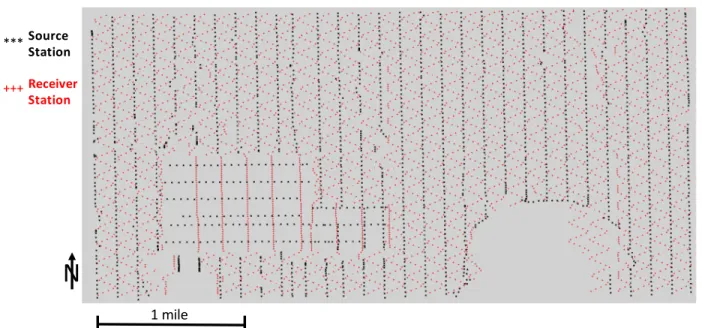
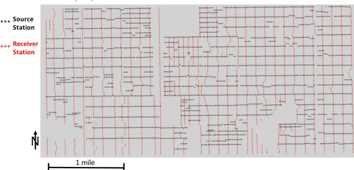
The two surveys I analyzed were acquired 3 years apart and cover an area of roughly 10 square miles. The term “legacy” comes in because the second survey (monitor) was not acquired following the geometry and parameters of the first survey (baseline), and the fact that they were not intended to the used for time-lapse analysis. The baseline was acquired using a geometry pattern called Lockhart Wave that was patented by Lockhart Geophysical (which acquired the seismic for APC). This geometry utilizes a north-south orientation for both source and receiver lines (Figure 3.1). The monitor was acquired using the conventional orthogonal pattern of source and receiver lines (Figure 3.2). The source lines were laid out west-east and the receiver lines were laid out north-south. During the acquisition, both surveys used different types and numbers of vibrators to generate the source. The baseline was acquired using 2 vibrators with a sweep frequency of 10-100Hz, while the monitor was acquired using 3 vibrators sweep 8-96Hz.
Figure 3.1. Acquisition geometry of the baseline survey using Lockhart Wave.
BASELINE (2010) 1 mile
N
Source Station *** Receiver Station +++Figure 3.2. Acquisition geometry of the monitor survey using a conventional orthogonal set-up. Differences caused by acquisition geometries/parameters need to be addressed during the co-processing to ensure and improve the 4D repeatability. First, because of the difference in the number of live channels during the acquisition, both surveys have different offset and azimuth distributions. The baseline has a maximum offset of 8000 feet with full azimuth distribution
Figure 3.3.Offset and azimuth distribution from both surveys
MONITOR (2013) 1 mile
N
Source Station *** Receiver Station +++ 7 7500 feet Offset Distribution Full Azimuth at 7500 feet Azimuth Distribution BASELINE (2010) 9500 feet Offset Distribution Full Azimuth at 11500 ft Azimuth Distribution MONITOR (2013)occurring within 7500 feet. In comparison, the monitor has a maximum offset of 18000 feet with full azimuth distribution occurring within 11500 feet of the offset. With the difference in
maximum offset, I anticipated a discrepancy in the number of traces going to each Common Depth Point (CDP). The fold maps (Figure 3.4 and Figure 3.5) show that the baseline has a maximum fold of 80, while the monitor has a maximum fold of 250.
Figure 3.4. Fold map of the baseline survey.
Figure 3.5. Fold map of the monitor survey. BASELINE (2010) 1 mile
N
22
23
24
MONITOR (2013) 1 mileN
22
23
24
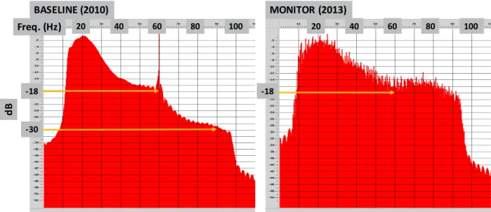
Second, the differences in the number of vibrators and the sweep frequency caused a discrepancy in the frequency content and amplitude. Figure 3.6 shows the amplitude spectra from both baseline and monitor calculated from the shot gathers. Both surveys have a peak frequency of 20Hz and both have a bandwidth from 10 to 60 Hz. The frequency of the baseline continues to diminish after 60Hz to around -30dB, while the spectrum of the monitor is
maintained at -18dB. It is also observable that the monitor covers more of the low frequencies compared to the baseline because the monitor was swept from 8Hz while the baseline was swept from 10Hz.
Figure 3.6. Amplitude spectra from both surveys extracted from the shot gather.
3.2 Co-Processing Workflow
Based on the observation in the previous section, I concluded that both surveys have low repeatability. To improve repeatability, I proposed the co-processing workflow laid out in Figure 3.7. Flows 2, 4, and 6 are the common processing workflows applied to both surveys. Using a common processing workflow and parameters is important to ensure that I do not introduce artificial differences in the time-lapse effects. In addition, I applied several
equalizations to handle the inherent discrepancy caused by the acquisition. Flows 1, 3, and 5 are the steps I took to improve repeatability by addressing the discrepancies. Flow 1 aims to tackle the discrepancy in the amplitude content. Flow 2 is intended to equalize both phase and
BASELINE (2010) MONITOR (2013) 20 40 60 80 100 20 40 60 80 100 -18 -18 -30 Freq. (Hz) dB
frequency in both surveys. Flow 3 accounts for the difference in source and receiver locations between surveys, and filters the number of traces based on proximity to minimize differences caused by any ray path discrepancy.
Figure 3.7. Legacy surveys co-processing workflow. Flows 2, 4, and 6 are the common
processing workflows, while 1, 3, and 5 are the equalization efforts to bring the monitor closer to the baseline.
The first investigation was conducted on the global amplitude content of both surveys (Flow 1, Figure 3.7). This process will bring the amplitudes of both surveys into the same range. The amplitude equalization was conducted using the Surface Consistent Amplitude
Compensation method, which calculates the RMS amplitude of both surveys and then calculates the scalar to be applied to both surveys. The amplitude calculation and scalar application are conducted with the raw data on the source and receiver domains. This is the first equalization done to balance amplitudes of both surveys and improve repeatability.
The following paragraphs briefly describe the common processing workflow applied to both surveys (Flow 2, Figure 3.7). Because of the land contours of the acquisition area, the elevations of the source and receiver locations are variable. To compensate for these variations, a constant datum needs to be assigned. A datum of 5500 feet was chosen so that the source and receiver elevations are located below the datum. Setting the datum above all the source and
Surface Consistent Amplitude Compensation 1stAmplitude Balancing
Attempt
Common processing flow includes: Datum Setting (5500 feet) Replacement Velocity (8000 feet)
Deconvolution
1stPass Velocity Picking (0.5 miles)
Refraction Static (V0 = 4000 ft/s) Noise Attenuation on each survey
Match Filter (Frequency and Phase Matching) 2nd Velocity Picking (0.25 miles) OVT-based trace Mapping and Sorting (4D Binning) Migration 1 2 3 6 5 4