MASTER THESIS IN
COMPUTER SCIENCE
30 CREDITS, ADVANCED LEVEL A2E
School of Innovation, Design and Engineering
Log-selection strategies in a
real-time system
Author
Niklas Gillström June 6, 2014 Advisor Dr Iain BateDepartment of Computer Science, University of York.
Visiting Professor at
School of Innovation, Design and Engineering, Mälardalen University. Advisor
Dr Patrick Graydon
School of Innovation, Design and Engineering, Mälardalen University.
Examiner
Prof. Sasikumar Punnekkat
School of Innovation, Design and Engineering, Mälardalen University
1
ABSTRACT
This thesis presents and evaluates how to select the data to be logged in an embedded real-time system so as to be able to give confidence that it is possible to perform an accurate identification of the fault(s) that caused any runtime errors. Several log-selection strategies were evaluated by injecting random faults into a simulated real-time system. An instrument was created to perform accurate detection and identification of these faults by evaluating log data. The instrument’s output was compared to ground truth to determine the accuracy of the instrument. Three strategies for selecting the log entries to keep in limited permanent memory were created. The strategies were evaluated using log data from the simulated real-time system. One of the log-selection strategies performed much better than the other two: it minimized processing time and stored the maximum amount of useful log data in the available storage space.
Keywords: Log-selection strategy, embedded real-time system, worst case execution time
overrun, bit error, deadline miss, Fault injection.
SAMMANFATTNING
Denna uppsats illustrerar hur det blev fastställt vad som ska loggas i ett inbäddat realtidssystem för att kunna ge förtroende för att det är möjligt att utföra en korrekt identifiering av fel(en) som orsakat körningsfel. Ett antal strategier utvärderades för loggval genom att injicera slumpmässiga fel i ett simulerat realtidssystem. Ett instrument konstruerades för att utföra en korrekt upptäckt och identifiering av dessa fel genom att utvärdera loggdata. Instrumentets utdata jämfördes med ett kontrollvärde för att bestämma riktigheten av instrumentet. Tre strategier skapades för att avgöra vilka loggposter som skulle behållas i det begränsade permanenta lagringsutrymmet. Strategierna utvärderades med hjälp av loggdata från det simulerade realtidssystemet. En av strategierna för val av loggdata presterade klart bättre än de andra två: den minimerade tiden för bearbetning och lagrade maximal mängd användbar loggdata i det permanenta lagringsutrymmet.
2
INDEX OF FIGURES
Figure 2.1.1 Dependability Taxonomy (Algirdas, Laprie, & Randell, 2001) ... 8
Figure 2.1.2 Simulated task pseudocode ... 9
Figure 2.2.1 An example algorithm with the order of n time complexity ... 10
Figure 3.4.1 Manipulation functions ... 18
Figure 3.5.1 Experimental setup ... 20
Figure 4.1.1 Simulated system ... 21
Figure 4.1.2 Task details format ... 22
Figure 4.1.3 Log-event format ... 23
Figure 4.1.4 Processor utilization factor ... 24
Figure 4.2.1 Worst Case Execution Time overrun ... 25
Figure 4.2.2 Bit Error on Period Began ... 26
Figure 4.2.3 Bit Error on Next Release ... 26
Figure 4.3.1 Fault injection results ... 29
Figure 4.3.2 WCET absorb ... 30
Figure 4.4.1 Strategy template ... 31
Figure 4.5.1 Strategy 1 pseudocode ... 32
Figure 4.6.1 Strategy 2 pseudocode ... 34
Figure 4.7.1 Strategy 3 pseudocode ... 35
Figure 5.1.1 Execution time of a whole simulation for log store sizes from approximately 4 KiB to 4 MiB. ... 37
Figure 5.1.2 Execution time of a whole simulation for log store sizes from approximately 8 MiB to 16 GiB. ... 37
Figure 5.1.3 Detected deadline misses at log store sizes from approximately 4 KiB to 4 MiB. ... 39
Figure 5.1.4 Detected deadline misses at log store sizes from approximately 8 MiB to 16 GiB. ... 39
Figure 5.1.5 Identified causes at log store sizes from approximately 4 KiB to 4 MiB. ... 41
Figure 5.1.6 Identified causes at log store sizes from approximately 8 MiB to 16 GiB. ... 41
INDEX OF TABLES
Table 4.1.1 Task details ... 22Table 4.1.2 Log-event variables ... 23
Table 4.1.3 Types of log entries ... 24
Table 5.1.1 Wilcoxon signed ranks test for hypothesis H1 ... 38
Table 5.1.2 Test statistics for hypothesis H1 ... 38
Table 5.1.3 Wilcoxon signed ranks test for hypothesis H2 ... 40
Table 5.1.4 Test statistics for hypothesis H2 ... 40
Table 5.1.5 Wilcoxon signed ranks test for hypothesis H3 ... 42
3
TABLE OF DEFINITIONS
The table of definitions describes the meaning of words and abbreviations used throughout the thesis. The page on which a definition is first used is also given.
Definition Description Page
Fault The cause to an error in a system. For example, code that results in an error.
5
Error The manifestation of a fault that causes an unwanted behavior of the system e.g. a worst case execution time overrun.
5
Failure The system is not performing according to the expected behavior.
5
Failure chain A chain of failures caused by faults in a system, which can lead to a failure and then to more failures.
5
NFF No Faults Found, i.e. could not identify the cause to a failure. 6
FPPS Fixed-Priority Preemptive Scheduling. 7
WCET Worst Case Execution Time, the maximum length of time a task or set of tasks requires to execute.
9
WCET overrun A task exceeds its maximum pre-defined execution time. 9
BEPB A Bit Error on Period Began. 9
BENR A Bit Error on Next Release. 9
WD Watchdog, an electronic timer to detect and recover from timing malfunctions.
22
Log-event A collection of variables in a fixed order. 23 log-file A static file with a finite number of log-events. 23
RAM Random access memory. 33
4
TABLE OF CONTENTS
ABSTRACT 1 SAMMANFATTNING 1 INDEX OF FIGURES 2 INDEX OF TABLES 2 TABLE OF DEFINITIONS 3 1 INTRODUCTION 5 1.1 Motivation ... 5 1.2 Purpose ... 7 1.3 Thesis statement ... 7 1.4 Thesis outline ... 7 2 BACKGROUND THEORY 8 2.1 Real-time systems ... 8 2.2 Big O complexity ... 102.3 Statistical hypothesis testing ... 11
2.4 Related work ... 13
3 SCIENTIFIC METHOD 15 3.1 Hypotheses ... 15
3.2 Instrument for measurement ... 16
3.3 Collection of empirical data ... 17
3.4 Manipulation of variables ... 18
3.5 Validation and analysis of data ... 19
4 DEVELOPMENT OF INSTRUMENT 21 4.1 System model ... 21
4.2 Instrument development ... 25
4.3 Validation of the instrument ... 28
4.4 Log-selection strategies ... 31
4.5 Strategy 1 ... 32
4.6 Strategy 2 ... 34
4.7 Strategy 3 ... 35
5 RESULTS 37 5.1 Execution time per simulation ... 37
5.2 Ability to detect deadline misses ... 39
5.3 Ability to correctly identify the causes ... 41
5.4 Threats to validity ... 43
6 SUMMARY AND CONCLUSIONS 46
7 FUTURE WORK 47
5
1
INTRODUCTION
1.1 Motivation
Software for embedded real-time systems is frequently engineered in accordance to an appropriate standard. Even if it is certified to conform to that standard, software might fail. Achieving adequate quality requires investigating these failures and improving the software where needed. In the system monitoring area, there is little research on planning logs to support the identification of the main cause of a failure/error, i.e. the initial fault. This is an important part of embedded real-time systems that needs more research, and important factors to minimize the defects that software can cause in a system. A time-consuming activity for developers of embedded real-time systems is manually finding the causes of failures that are reported by their users; thus it is important to have valid scientific results that can help in deciding which logging strategies are more optimal. Since it is hard to perform a scientific experiment necessary for evaluating the different logging strategies in a real system due to its high complexity, a simulator based approach was used.
In order to determine the most optimal log-selection strategy, both failures and their causes need to be found, which comprises a series of events (Algirdas, Laprie, & Randell, 2001). Fault is the cause of an error in a system. Error is the manifestation of the fault that causes an undesirable behavior of the system. Failure is when a system is not performing according to the expected behavior. A failure chain is a chain of failures, which are faults in a system that lead to a failure, which in turn leads to more failures. There are a number of combinations of faults that can result in failures. The types of faults in the timing domain for tasks are the following: a task finishes too early, a task finish too late, and task omission.
Tracing an error to its initial fault before it results in a failure requires identifying errors and investigating their causes. Identifying faults from log data requires that sufficient information has been logged (Laprie, 1995). The amount of log data that can be kept is limited due to an embedded system’s limited storage space. Filtering logs is constrained by a system’s processing power. These limits necessitate optimizing what log data is kept. With minimal resources in an embedded real-time system, it is not feasible to detect faults during
6
run-time by the real-time system scheduler, which comes at the cost of increased processing power and time.
To identify the root-cause of an error, three steps need to be performed: detect the unwanted behavior, categorize that behavior, and finally identify what caused the detected behavior. Detecting unwanted behavior is easier than identificaton of what caused the behavior.
The difference between detection and identification of the root-cause of an error can easily be misunderstood. The difference can be explained through the following example: A failure is detected in task t2 through the observation of a deadline miss, which means we know
something happened. Then a software related failure that caused a deadline miss is noticed, which means we now know what happened. On further examination of log data, a worst case execution time overrun is observed in task t1, which did run before task t2 that missed its
deadline. One can then identify that task t1 caused the deadline miss in task t2 by the worst
case execution time overrun.
An error needs to be detected in order to be identified, and one technique is described in (Mok & Liu, 1997), which was to use a constraint violation technique for error detection. In their work, they set a number of constraints and implemented a JRTM (Java Run-time Timing Constraint Monitor) with low overhead, which they claim can catch any violations of the specified timing constraints.
Accurately identifying the cause of a failure is difficult. Today, investigation often reports No Faults Found (NFF). NFF implies that a failure did occur during the execution of a program, and that a failure or fault could not be found when analyzing the cause of the failure. NFF is by far the most common outcome of investigation, and airlines voted this “the most important issue” (Burchell, 2007). According to recent studies (Hockley & Phillips, 2012), NFF is still the most common outcome of investigations. Investigating how to choose what to log in an offline system could provide insights on how to detect more dangerous faults, reducing the incidence of NFF.
A study that would take all possible failures and faults into consideration would have infeasible complexity. The faults and failures investigated in this study are worst case execution time overruns, bit errors in release time calculations, and deadline misses. We leave extending this work to other faults and failures to future work.
7
Furthermore, it would not be feasible to monitor all types of faults and log these, due to the limited resources available in an embedded real-time system (Avizienis, Laprie, Randell, & Landwehr, 2004). This would require constant monitoring and logging even when no failures are present in the embedded real-time system. There is also a possibility that a worst case execution time overrun does not result in a deadline miss. Logging all activity to find these would require more log-file space and processing power than is available in real systems. A more feasible strategy is to log only a set of Real-Time Operating System (RTOS) events and system calls selected to maximize the chance of capturing details that identify the fault.
A commonly used scheduling algorithm in embedded real-time systems is Fixed-Priority Preemptive Scheduling (FPPS), which means that research based on it will provide insight into other systems that use FPPS. In the FPPS algorithm, the scheduler guarantees that the processor executes the task that has the highest priority of all tasks that are available for execution at any given time.
1.2 Purpose
The purpose of this study is to determine what data should be logged in an embedded real-time system while still being able to accurately identify the cause of an error from the saved log data. An optimum strategy for achieving this is devised.
1.3 Thesis statement
The problem that needs to be solved is selecting a highly effective way to determine what data should be logged so as to maximize the chance of accurately identifying the cause of the error from the log data. Embedded targets usually have limited resources available for storing log files or processing log entries. At first we assume there are minor resource limitations in order to be able to create a general method that works, and then look to optimize the resource usage. We are also simultaneously trying to optimize the resource usage to store the largest amount of useful data using the least amount of space.
1.4 Thesis outline
The rest of the thesis is organized as follows. Chapter 2 presents the theory needed for understanding the basics of the thesis. Chapter 3 describes the method used to conduct the study in a structured and reliable way. Chapter 4 describes how the instrument was created and its accuracy validated. Chapter 5 presents the results and reflections on the results in relation to the presented problem. Chapter 6 presents a summary of the research, conclusions made and explanations of hypotheses. Chapter 7 discusses directions for future work.
8
2
BACKGROUND THEORY
The purpose of the background is to provide sufficient information for the reader to understand key concepts dealt with in the rest of the thesis. Big O complexity describes the limiting behavior of functions used in this paper which have trends that move towards infinity. Real-time system aims to explain the fundamentals of a real-time system. Statistical hypothesis testing explains the basics of the hypothesis testing used in the thesis.
2.1 Real-time systems
Real-time systems are systems that must respond within a finite and specified period of time. It is not the speed that characterizes a real-time system, but the predictability. In order to have a predictable real-time system, each task has to provide a correct response within its timing constraints.
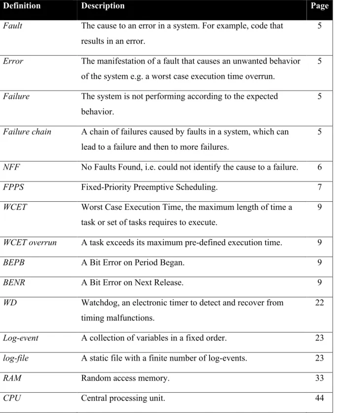
FIGURE 2.1.1 Dependability Taxonomy (ALGIRDAS, LAPRIE, & RANDELL, 2001)
Figure 2.1.1 shows the area this study is focusing on, i.e. threats in the dependability taxonomy (Algirdas, Laprie, & Randell, 2001). Faults, Errors, and Failures relate to the other aspects of dependability in a number of different ways. However, this study’s focus is threats and how to identify and store them using minimal resources.
The scheduler controls the queue of tasks to be executed in a real-time system. In FPPS, every task has a fixed priority. The execution order for tasks is determined by their priority, which is usually assigned before run-time. A task with higher-priority preempts a lower-priority task. When a task gives up the processor or is preempted, a context switch occurs. These context switches are an execution time overhead (Zmaranda, 2011).
Preemption is when a higher-priority process takes control of the processor from a lower-priority task (Hang, 2010). A job is considered preemptible if its execution can be suspended
9
to switch the execution to other jobs and later resume from where it was interrupted. With priority-based scheduling, a high-priority task can be released when a task with lower priority is executing. When a preemptive scheme is used, the system can quickly switch to the higher-priority task, making high higher-priority tasks more responsive.
Context switching overhead means that it takes a finite amount of time for the operating system to switch between two jobs. This is an overhead for the scheduler. If jobs are switched often, the context switching overhead becomes a significant factor as it decreases the predictability of a real-time system (Zmaranda, 2011).
A task is a schedulable unit of processing consisting of one or more actions. A task is usually implemented as a process or a thread (Ramaprasad, & Mueller, 2011). A task has a number of attributes. The Worst Case Execution Time (WCET) is the longest allowed undisturbed execution time for one iteration of the task. Period is the interarrival interval for a sequence of periodic events. Offset is the earliest time instant at which the task becomes executable.
FIGURE 2.1.2 Simulated task pseudocode
Figure 2.1.2 shows the pseudocode for a simulated task. A task contains a number of lines of code or a set of functions that executes in a predefined order. A task could have any of a number of kinds of faults. When faults occur they can cause a task to miss its deadline. In order for a real-time system to work as expected, the deadline of all tasks must be met.
The faults we inject are WCET overruns, Bit Error on Period Began (BEPB), and Bit Error on Next Release (BENR). WCET overrun occurs when a task executed longer than expected. Deadline miss occurs when a periodic task
10
executes beyond next_deadline. The injected fault BEPB represents a fault in the calculation of period_began in the pseudocode, which the scheduler uses initially in the task function and in the end of each iteration of the infinite loop.
The injected fault BENR represents a fault in the calculation of next_release in the pseudocode, which the scheduler uses initially and at the end of each iteration of the infinite loop. This means that the scheduler will release the affected task at the wrong simulated time.
2.2 Big O complexity
Big O notation is used to estimate the worst time or space complexity for an algorithm. Complexity is the efficiency of an algorithm, how the algorithm scales when input size n increases (Garey & Johnson, 1979). In our context, input size n is the total number of log entries processed by a strategy. Variables with constant values do not depend on input size n and are thus omitted. As only the worst case is considered, magnitudes less than the worst case magnitude are omitted. Space complexity is storage space required on a flash memory or other storage related medium to store the values. In this thesis, this is equal to a fixed-size buffer on flash memory storing m values from the input size n. Output size m is the total number of log entries written to the fixed-size buffer on flash memory by a strategy. Space complexity is also the working space in RAM that the algorithm requires to store the values for input size n, where n is the size of the in RAM buffer used for logging by a strategy. Time complexity is how much time the algorithm requires to run as a function of the size of the input (Tarek, 2007). In this thesis, it means the required execution time for a strategy to fill a fixed-size buffer on a flash memory.
FIGURE 2.2.1 An example algorithm with the order of n time complexity
Figure 2.2.1 demonstrates 𝑇 𝑛 ∈ 𝑂 𝑛 the algorithm has the order of n time complexity, which is the same as the algorithm taking linear time to run relative to its input size n. Input size n is the total number of log entries processed by a strategy. Among other used complexities in this thesis is 𝑆 ∈ 𝑂 1 , the algorithm has order of 1 space complexity,
11
which is the same as the algorithm using constant space to store values relative to its input size n.
𝑇 ∈ 𝑂 𝑛 time complexity means minimal resource usage in terms of processing power, where n is the number of processed log-events. However, one could claim that the practical time complexity is 𝑇 ∈ 𝑂 𝑐 , where c is the constant execution time required to process a log-event. This claim is true when log-events are delivered incrementally by a scheduler instead of being delivered all at once to a strategy as in this experiment. 𝑇 ∈ 𝑂 𝑐 is true because the instrument is processing a task’s log-events in a loop, when applied as a filter it executes in constant time since the loop is then in the scheduler.
Choosing what to log in limited space is related to Big O complexity since the working space complexity is 𝑂(𝑛) using minimal resources in terms of the in-RAM buffer, where n is the number of processed log-events. However, this is not related to the number of log-events stored simultaneously. A strategy needs to process all log-events in order to be helpful in identifying dangerous faults; otherwise a vital log-event can be missed. The minimal complexity for the number of simultaneously stored log-events in a strategy is 𝑆 ∈ 𝑂 𝑐 , where c is a constant storage space of log-events and used variables in the in-RAM buffer.
2.3 Statistical hypothesis testing
An experiment has both Independent Variables (IV) and Dependent Variables (DV). The IV is manipulated by the researcher, and the DV gets influenced by changes in the IV. The IV is the cause and the DV is the effect.
A hypothesis is a claim or statement about a property of a population (Javanmard & Montanari, 2013) made from observing a sample. One or more significance tests can be conducted for one hypothesis, to provide additional evidence against the null hypothesis. In order to use a hypothesis to support a claim, the claim can be formulated using negation in the null hypothesis, so its inverse becomes the alternate hypothesis. In this study, hypothesis testing is used to support the alternative hypothesis. The rejection of a null hypothesis does not mean it is false; it shows either the probability of a type I error or the probability that it occurred by chance alone.
12
The significance level when a test is considered to be statistically significant can be expressed as the probability that the rejection of a null hypothesis is a mistake (Cox, 2008). The probability that an event occurred by chance is called p-value where the p-value must be less than or equal to the hypothesis test value to reject the null hypothesis. The p-value in this study is 0.01 which is a commonly used value. The value 0.01 is equal to 99% confidence that this result did not simply happen by chance. In decision theory, it is the opposite, so it is interpreted as the probability of the rejection that the null hypothesis is a mistake. The probability of a Type I error is equal to the significance level alpha (α).
A test of significance starts by first defining a null hypothesis H0 and then an alternative hypothesis Ha. The null hypothesis H0 represents a theory that has been put forward to be used as a basis for an argument that has not yet been proven. The formulation of the null hypothesis H0 is the most important and usually implies zero or no change when the subject of the study is an intervention. The null hypothesis H0 always includes the equal sign, which is ≤, =, or ≥. The decision to reject or accept is based on the null hypothesis H0. The alternative hypothesis Ha statement is most likely to be true if the null hypothesis H0 is false. There exist multiple null hypotheses in this problem: 𝐻!, 𝐻!, … , 𝐻! and the alternative hypothesis Ha. The type of tail-test is two-tailed when the null hypothesis is written with only an equal sign and is one-tailed when the null hypothesis includes ≤ or ≥.
Wilcoxon Signed Rank Test is a nonparametric alternative for paired sample t-test (Wilcoxon, 1945). It is used for comparing data from paired sample. It does not require the data to be normally distributed. Paired data is data that has a one-to-one relationship between values in the two data sets. Each data set needs to have an equal amount of observations and each data point can only be related to exactly one observation in the other data set. The mean rank indicates the direction of change, an example of this is when a negative mean rank from an initial measure is less than a positive mean rank of an additional measure. This suggests that the measured values from the last observation is most likely higher than the measured values from the first observation (Motulsky, 2013).
A Wilcoxon Signed Rank Test evaluates the difference between observations using a before and after approach. Positive ranks indicate that values after are most likely higher than before, and the opposite for negative ranks. The test results should be fairly accurate when the sample size is 16 pairs or greater (Wilcoxon, 1945). A sample size of 23 pairs is used in this study.
13
2.4 Related work
There seems to be little research on planning logs to support the identification of the main cause of a failure. However, there are a few similar studies in the area of detecting and identifying timing related errors. In one of the studies, a software monitor is created by following the requirement documentation, which according to the author (Peters, 2000) is for a realistic system. It was discovered that the generated software monitor was able to detect undetected errors in prior tests. A technique called transformation modes to specify anomalies that are allowed from the normal actions is used. Although their used approach is not directly applicable to this thesis because we focus on offline evaluation and they focused on online evaluation, the study still gives good insight on how to design a monitor that can be used when detecting failures in a log file.
The study gives a good insight on how to design a monitor that can be used when detecting failures in a log file, although their used approach is not directly applicable to this study because we focus on offline evaluation and they focused on online evaluation.
Another paper with an interesting approach that might be of use when designing the tools in this study is the research performed by (Mok & Liu, 1997), where a language for specifying timing constraints was created. Using specification in that language in combination with an algorithm for monitoring, they were able to capture anomalies in the development phase. They achieved this by first compiling the specifications of the constraints into run-time system monitoring software. In (Pettersson & Nilsson, 2012), the monitoring is done in a different way, but contains an interesting approach for using buffers. The concept of capturing violations at run-time (Mok & Liu, 1997) is an approach that could be used if sufficient resources are avaliable. A big difference from this study is that their work assumes the availability of many timers.
To understand different aspects of how a deadline miss can occur in a task set, the insight from (Regehr, 2002) is of interest, especially the comparison between preemptive and non-preemptive task sets. Their research revealed that WCET overruns are more likely to cause a deadline miss when using preemptive scheduling compared to non-preemptive scheduling. That increased the confidence to use FPPS as the intention is to investigate FPPS and inject WCET overruns in this study. The illustrations in their paper show the importance of checking that the scheduling parameters have been properly configured when setting up task sets in order to increase the validity of the experiment results. Their work
14
differs in a number of ways from this study: their aim is to make non-preemptive task clusters and they inject 50% release jitter. However, the algorithms created in their work were taken into account when creating the validation algorithm to make the instrument in this study more robust.
There are several studies in mutation testing that are relevant to this study. Several empirical studies (Anand, et al., 2013) show that failure-causing inputs and nonfailure-causing inputs tend to form continuous blocks. This is particularly valuable knowledge when designing the log-selection strategies: it can result in strategies with more relevant data in its buffers. However, the most interesting part of their research is the Adaptive Random Testing (ART) which takes into account the vast number of manifestations a fault can have examined.
Jia & Harman present a comprehensive survey of mutation testing research that covers a wide range of theories including equivalent mutant detection and techniques for optimization (Jia & Harman, 2011). Regression testing in particular is a good approach to reduce the size of a test set. Some empirical studies showed that a 33% decrease in number of test sets was possible without any loss of effectivity. This was taken into account during the selection of what should be logged when optimizing the strategies.
The paper by (McMinn, 2004) contains many interesting parts related to this study in several ways by using a number of techniques. Execution Time Testing will be used during the development of the instrument for measurement. There exist a number of other interesting techniques; the fundamentals of Search-based Execution Time Testing and the Chaining Approach could be used offline when finding causes to deadline misses. This is taken into account when creating the validation algorithm.
Assertion Testing (McMinn, 2004) and Exception Condition Testing (McMinn, 2004) techniques can be used to make the instrument for measurement more robust when developing, and it results in higher quality of the code of the instrument by using a kind of exception handling. For testing timing behavior, Execution Time Testing and Search-based Execution Time Testing (McMinn, 2004) will be considered in this study.
15
3
SCIENTIFIC METHOD
An initial perception of the problem was divided into three hypotheses to be accepted or rejected. This chapter explains the method used for conducting the experiment.
3.1 Hypotheses
The problem statement is divided into three claims comprising multiple null hypotheses and an alternative hypothesis for each claim. The hypotheses are related to choosing what to log so as to retain log records in a limited space that will be most helpful in identifying faults by validating collected data for determining the existence of an optimal log-selection strategy. Each hypothesis will provide support for the optimal strategy in relation to what is tested. The proposed hypotheses will focus on: execution time per simulation (H1), ability to detect deadline misses (H2), and ability to correctly identify the causes (H3). Strategy 1 stores everything, strategy 2 stores fewer types of log events than strategy 1, and strategy 3 stores the least types of log events. Section 4.5 - 4.7 provides a more detailed description of the strategies.
Hypothesis H1 is that strategy 3 requires the least execution time at each log store size.
H10: Strategy 1 mean rank ≥ Strategy 2 mean rank.
H11: Strategy 3 mean rank ≥ Strategy 1 mean rank.
H1a: Strategy 3 mean rank < Strategy 1 mean rank < Strategy 2 mean rank.
A rejection of the null hypotheses H10 and H11 indicates that the mean rank for strategy 1 and 2 is higher than the mean rank for strategy 3. This means the rejections provide support that strategy 3 is executing simulations in significantly less time than strategy 2 and strategy 1. If H10 is rejected it means that strategy 2 is executing simulations in significantly more time than strategy 1. If both H10 and H11 are rejected it means that strategy 1 is executing simulations in significantly more time than strategy 3. Thus, strategy 2 also executes in more time than strategy 3. Hypothesis H1 is related to the goal of using the least practical amount of processor resource on the embedded target.
Finding more deadline misses with one or more identified causes relates to how well a strategy stores the most relevant log data in the permanent storage. Thus, hypothesis H2 is
16
related to the goal of not requiring more permanent storage resource on the embedded target by being more efficient in the selection of log data to commit.
H20: Strategy 2 mean rank ≤ Strategy 1 mean rank.
H21: Strategy 3 mean rank ≤ Strategy 2 mean rank.
H2a: Strategy 3 mean rank > Strategy 2 mean rank > Strategy 1 mean rank.
A rejection of the null hypotheses H20 and H21 indicates that the mean rank for strategy 1 and 2 is higher than the mean rank for strategy 3. This means that strategy 3 stores significantly more log data relevant to deadline misses than strategy 1 and strategy 2. If H20 is rejected it means that strategy 1 stores significantly more log data relevant to deadline misses than strategy 2. If both H20 and H21 are rejected it means that strategy 2 stores significantly more log data relevant to deadline misses compared to strategy 3. Thus, strategy 3 also stores significantly more log data than strategy 1.
Hypothesis H3 is that strategy 3 identifies the most injections in all simulations. A rejection of the null hypotheses H30 and H31, means that the mean ranks for strategy 1 and 2 are higher than the mean rank for strategy 3. This means that strategy 3 identifies significantly more injections than either strategy 1 or strategy 2.
H30: Strategy 2 mean rank ≤ Strategy 1 mean rank.
H31: Strategy 3 mean rank ≤ Strategy 2 mean rank.
H3a: Strategy 3 mean rank > Strategy 2 mean rank > Strategy 1 mean rank.
If H30 is rejected it means that strategy 1 identifies significantly more injections than strategy 2. If both H30 and H31 are rejected it means that strategy 2 is identifying significantly more injections than strategy 3. Thus, strategy 3 also identifies significantly more injections than strategy 1. Hypothesis H3 is related to the goal of selecting the log entries that contain the most useful information in terms of finding faults which enables optimizing of the resource usage in order to store an optimal set of log data.
3.2 Instrument for measurement
The instrument for measurement is the tool created for collecting and assessing the experiment data. The log-selection strategies were validated by creating a tool for analyzing a log to find faults revealed by its entries. Firstly, the instrument for measurement were
17
validated to confirm reliable identification of the injected faults, secondly after the accuracy of the instrument was determined, existing anomalies and their measured effects were explained in detail to increase confidence in the instrument.
3.3 Collection of empirical data
The simulator generates two files per test, where the first file contains the task parameters, and the second one contains the log data from the simulated real-time system run. To validate the reliability of the instrument, for each of the ten tests the two files were read in by the instrument. Later, twenty-three additional sets of test data were generated to evaluate the log-selection strategies using the instrument. We used the log files from a single test run to test each of the three strategies, with the intent to provide a fair comparison between the log-selection strategies.
The data collected to test hypothesis H1 is the execution time needed to run each log-selection strategy over an entire log-file and then analyze the selected log entries using the instrument. We measured this at different log sizes. Thus, execution time is the dependent variable and the independent variable is the size of the log store. Hypothesis H1 and the collected data are related to the goal of using the least practical amount of processor resource on the embedded target rather than an on-line fault detection strategy such as WCET monitoring.
The data collected to test hypothesis H2 is the number of deadline misses found to have one or more identified causes. We measured this at different log sizes. Thus, the number of found deadline misses with one or more identified causes is the dependent variable, and the fixed-size number of log-events is the independent variable. Hypothesis H2 and the collected data are related to the goal of not requiring more permanent storage resource on the embedded target by being more efficient in the selection of log data to commit.
The data collected to test hypothesis H3 is the number of injections the instrument correctly identified in the log data selected by each strategy. We measured this at different log sizes. Thus, the number of injections found is the dependent variable, and the fixed-size number of log-events is the independent variable. Hypothesis H3 and the collected data are related to the goal of selecting the log entries that contain the information that reveals the most faults. Testing hypothesis H3 facilitates storing an optimized subset of log data.
18
3.4 Manipulation of variables
The independent variable in all three cases were expressed by the number of log-events of a fixed-size buffer on flash memory. The independent variable was manipulated by increasing its size logarithmically. The dependent variable of the first test was the execution time, in the second test the dependent variable was the number of deadlines misses with identified cause(s), and in the third test the dependent variable was the number of correctly identified injections.
FIGURE 3.4.1 Manipulation functions
Figure 3.4.1 shows the functions used to reduce the noise. A sample manipulation was performed on the collected data. The sample manipulation procedure taken to reduce the noise was for smoothing all measured DV values per log store size. The noise was caused by the limited accuracy of the execution timing mechanism, and the simulator’s use of a random number generator. We limited each sample to the range the arithmetic population mean (A) ± Standard population Deviation (SD). We then computed the A of the adjusted data for each log store size and strategy. The effect on the outlier values was that each outlier value was replaced with an adjusted value, which resulted in minor differences to the A. The pre-processing of the measure values was necessary in order to minimize outliers/noise. The returned values of the A were rounded to two digits of precision in the execution time tests and in the number of found deadline misses with identified cause(s) tests, the mean was rounded to the closest integer.
19
3.5 Validation and analysis of data
The collected data were validated in a number of steps. The first step was to validate all simulator generated files by comparing the task parameter information in the console window of the simulated system with the task parameters in the generated files.
The second step was to validate that the log data had the correct format by reading the binary data into the instrument. The accuracy of this method is robust because the execution of the instrument would be interrupted if a single parameter were in the wrong format. The data were pre-loaded into the instrument, and once data was loaded the measurements were manually started. Hence, the startup time of the instrument did not affect the results.
The third validation step was to compare the data to the ground truth. The injected faults were divided into groups related to their ground truth. The results of each group were divided into signal detection metrics excluding true negatives that were the normal execution path.
IBM SPSS Statistics Professional Edition v.22 was used to conduct Wilcoxon Signed Ranks Tests. The purpose of using the Wilcoxon Signed Ranks Tests was to get before and after comparisons. This relates to the strategies since strategy 2 was based on strategy 1 and later optimized, and strategy 3 was based on strategy 2 and later optimized. Since the purpose was to compare a limited number of significance tests, a planned comparison (Motulsky, 2013) was conducted, which means that there were no correction for multiple comparisons.
To validate the analysis of all hypotheses, one-tailed significance level alpha (α) = 0.01 was used in Wilcoxon Signed Ranks Tests. The type of test was for paired data, which is when a one-to-one relationship exists between values in the two data sets. Each data set needs to have an equal amount of observations and each data point can only be related to exactly one observation in the other data set.
This is an experiment because of the study method, and the subject is partially related to algorithms and complexity, whose complexity class is NP-easy (Garey & Johnson, 1979). Standard procedures (Swales & Feak, 2004) were used to organize the experiment. The reason for the focus on complexity was the creation of algorithms that needed to be tested.
20
Asymptotic algorithm analysis was used to determine the processing time of the log-selection strategies in big O notation. First, the worst case number of executed primitive operations that executed as a function of the input size was found.
Next, the constant factors and lower-order terms were disregarded when counting primitive operations, simple operations that can be performed in constant time. Finally, the exact number of array accesses made in the algorithm in asymptotic notation of the function was expressed with big O notation. Asymptotic algorithm analysis was used to determine the working space requirements of the log-selection strategies in big O notation. The working space requirements comprised the in-RAM buffer and flash storage space.
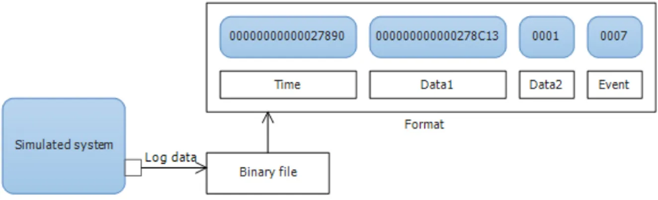
FIGURE 3.5.1 Experimental setup
Figure 3.5.1 demonstrates the setup that was used in the experiment. The system simulator used in the experiment was already existing. The instrument for measurement, the binary files, and the log-selection strategies were created by the author. It would be optimal to perform the experiment in a real embedded real-time system because it would be more complex and might perform differently than the simulated system used. However, the use of a simulator has a number of benefits compared to a real system. The use of a simulated system enabled direct and detailed observations for evaluating log-selection strategies. A simulated system with fewer required restrictive assumptions reduced complexity. Immediate changes in the structure and configuration of the simulated system were possible. Small changes to the simulator were made in order to save log data to a binary file.
21
4
DEVELOPMENT OF INSTRUMENT
The experimental instrument was created based on the requirements of the study. We then validated that it worked as expected. The experiment on the log-selection strategies were conducted after the instrument had been validated. In the following sections, we explain further details on the instrument development validation and log selection strategies.
4.1 System model
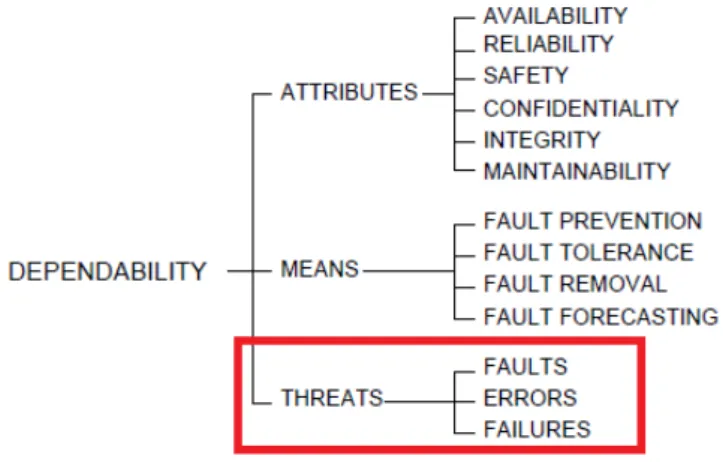
FIGURE 4.1.1 Simulation of failure behaviours in an embedded real-time system
Figure 4.1.1 illustrates the simulation of failure behaviors in an embedded real-time system. Three faults were injected: WCET overrun, which occurs when a task executed longer than expected; BEPB which occurs when a randomly-selected bit in the calculated period_began is flipped as illustrated in Figure 2.1.2; and BENR, which occurs when a randomly-selected bit in the calculated next_release is flipped.
Simulation attributes: • Error o Deadline miss • Faults o WCET overrun o BEPB o BENR
22 • Scheduler
o FPPS algorithm
o Non-blocking for higher priority tasks o Small amount of slack time
o Watchdog (WD)
o Context switch overhead o Periodic tasks
We used the simulator system to create a static log-file containing all possible entries that we examined using the instrument. The log-file with log entries was first pre-loaded into the instrument; when completed the file with task details was also read by the instrument. Once the instrument loaded both files, the measurements were manually started by the engineer. The filtering is performed by the instrument.
TABLE 4.1.1 Task details
TID BCET WCET PERIOD OFFSET DEADLINE PRIORITY
0 45 50 500 10 550 0
1 95 100 825 0 1000 2
2 530 550 825 0 1000 3
3 95 100 1000 825 1000 1
Table 4.1.1 shows the task details that were used in all tests. The time units represent the simulated system's clock in ticks of unspecified duration. Task ID (TID) uniquely identifies each task. Best Case Execution Time (BCET) gives the lower bound of the execution time. WCET gives the upper bound of the execution time. Actual execution time of each job was a random number selected from the uniform distribution (BCET, WCET). The remaining columns show each task’s period, offset, deadline, and priority. The simulated system recorded these details to a details file for use during the experiment and later analysis.
23
Figure 4.1.2 demonstrates the structure of the format used in the static task details file. The details from task id 1 were used in this illustration, and a translation from decimal to hexadecimal was performed.
TABLE 4.1.2 Log-event variables
VARIABLE DATATYPE DESCRIPTION
Time UINT64 The simulated system's clock in ticks of the duration specified in a task set.
Data1 UINT64 Keep different values of time or 0.
Data2 UINT16 Task ID.
Event UINT16 The type of log entry.
Table 4.1.2 shows the format of a log-event. The meaning of data1 and data2
depend on the type of log event as shown in
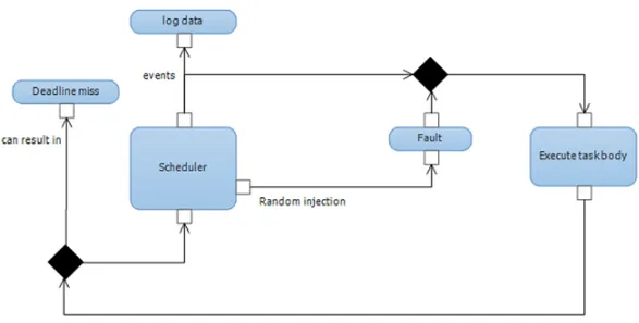
Table 4.1.3. The simulated system generated two binary files: the details file and a file containing log data. The log-file represents the unfiltered log output of a simulation run as a sequence of log events. Each log-event comprises four variables: the time at which the entry was generated, data1 which stored a number of different timing entries, data2 shows to which task id the event is for, and event which shows the type of log entry. Each log-event record has a size of 20 bytes.
FIGURE 4.1.3 Log-event format
Figure 4.1.3 illustrates the structure of the format used in the static log-file. In the original data, there were eight pairs of hex characters in time and data1 respectively, which were equal to 8 bytes each. Data2 was two pairs of hex characters and the event was also represented by two pairs of hex characters. The data were originally in binary format that was translated in order to be illustrated in a humanly readable format.
24 Table 4.1.3 Types of log entries
TYPE DESCRIPTION
Task create The task with ID data2 has been created and will begin its first period at data1.
Task wait The task with ID data2 has called the simulated wait_until_offset function as shown in Figure 2.1.2 to wait until the time data1.
Task sleep The system has no runnable tasks and will be going to sleep until waking up at data1 to run task with ID data2.
Task release The task with ID data2 has been released. If it was waiting on a simulated wait_until_offset call, data1 gives the time it was waiting until. If not, data1 is 0.
Task switch The scheduler is switching to the task with ID data2. Data1 is 0.
Task return The task with ID data2 has returned from the simulated wait_until_offset call it used to wait until the offset for the period beginning at time data1.
Task dlmiss The periodic task with ID data2 self-reported that it has missed its deadline for the period beginning at time data1.
WD
running The watchdog was running. Data1 and data2 are 0.
WD restart The watchdog timer restarted the task with ID data2; it will run at or after time data1.
Table 4.1.3 illustrates the types of events logged by the simulated system. Within one time span there were the following types of log entries: task create, task release, task sleep, task switch, task return, task dlmiss, task wait, WD running, and WD restart. All log entry types other than task create occured at some occasion within the time span between two releases of a task regardless of its task id. Task create only appeared once per task and test.
𝑈 = 𝐶! 𝑇! !
!!!
FIGURE 4.1.4 Processor utilization factor
Figure 4.1.4 shows the formula for processor utilization factor where Ci was the worst case execution time and Ti the period of its task. In the simulated system, four tasks were running in a simulated real-time operating system with details as in Table 4.1.1. No deadline misses were caused by the processor utilization factor since it was less than one
25
(0.1+0.12+0.67+0.1=0.99). The simulated system was sensitive and had only a small amount of slack time. This made it more vulnerable to injections; that is, injections were likely to produce deadline misses, including misses in other tasks and in subsequent jobs.
4.2 Instrument development
We tested the instrument by simulating execution for 40,000,000,000 cycles while randomly injecting faults. An initial validation algorithm was created to identify as many injections as possible. We tested using a range of fixed-size buffers between approximately 4 KiB and 16 GiB. We made 10 simulations for each buffer size to increase the number of measurements. The generated truncated logs were examined and validated against the ground truth. We smoothed all measured values by limiting their upper and lower values to the A ± SD.
Two test sets were created to ensure that the results were not isolated incidents. The first test set was for assessing how accurately the instrument for measurement could identify the injected faults. The second test set was for testing how optimal a strategy performed to save sufficient data while still being able to identify faults that inflicted a deadline miss.
2013-‐12-‐05 2014-‐06-‐05 2014-‐01-‐01 2014-‐02-‐01 2014-‐03-‐01 2014-‐04-‐01 2014-‐05-‐01 2014-‐06-‐01 WCET overrun Task Cycle T2 Task Release Time Task Deadline Execution Time T1
FIGURE 4.2.1 Worst Case Execution Time overrun
Figure 4.2.1 demonstrates a WCET overrun, which occurred when a task executed longer than its WCET (e.g. T1). The instrument evaluated whether the log messages showed
the task executing for longer than its specified WCET at time T1 or not. If a task executed
longer than T1 and finished execution at the time T2, the instrument reported a WCET
26 2013-‐12-‐05 2014-‐06-‐05 2014-‐01-‐01 2014-‐02-‐01 2014-‐03-‐01 2014-‐04-‐01 2014-‐05-‐01 2014-‐06-‐01 Bit Error Task Cycle Task Deadline T1 Task Release Time Execution Time T2 Period Began
FIGURE 4.2.2 Bit Error on period began
Figure 4.2.2 shows the concept of a BEPB. The scheduler got a bit error at T2 in the
period began calculation referring to T1. The error could occur at two locations, either in
the beginning of the task function which takes the initial period as period began, or during the calculation of next release.
In the simulated system, bit errors had a big impact on when a task asked to be woken up. A bit error occurs when a bit is flipped, switching a bit from 1 to 0 or 0 to 1. The effect on execution time depends on which bit was flipped. If a task effectively stopped executing due to a bit error, the simulated system’s watchdog would eventually notice and restart the task.
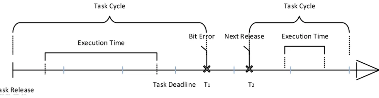
2013-‐12-‐05 2014-‐06-‐05 2014-‐01-‐01 2014-‐02-‐01 2014-‐03-‐01 2014-‐04-‐01 2014-‐05-‐01 2014-‐06-‐01 Next Release Task Cycle Task Deadline T2 Task Release Time Execution Time T1 Task Cycle Execution Time Bit Error T2 Figure 4.2.3 Bit Error on next release
Figure 4.2.3 illustrates the concept of a BENR. The scheduler got a bit error at T1 in the
next release calculation referring to T2. The error could occur in the reoccurring
calculation that were period began + offset of the task to produce its next release value. When a bit error occurred at this point, the count for BENR injections were increased.
27
Test set specifications:
• Instrument test set – 1 % injections of WCET overruns, BEPB and BENR to evaluate if the instrument could identify the injected faults correctly in a log containing all possible entries. A simulated execution ran for 40,000,000,000 cycles. The task
parameters used were the same in all of the ten tests.
• Log test set – 1 % injections of WCET overruns, BEPB and BENR to evaluate the log-selection strategies. Each simulated execution ran for 40,000,000,000 cycles. The task parameters used were the same in all of the twenty-three tests. Twenty-three tests were chosen since it reflected the logarithmically increasing log store size, and where the 23rd test was closest to the physical limits of the hardware used.
The differences between fault, error and failure were important: engineers examine logs to find the true cause of field failures. In some cases, failures related to a chain of faults and errors that resulted in a failure. The relationship between fault, error and failure is the following: faults can result in errors and errors can lead to failure. In general, failures can only exist after an error occurred, and an error can only exist after a fault occurred.
The assumed page size was 4 KiB. The sizes of all fixed-size buffers on flash memory for logging were a multiple of the page size. We measured the dependent variable for each hypothesis at a range of buffer sizes from approximately 4 KiB to 16 GiB, distributed logarithmically.
Since the flash memory writes an entire page at a time, the simulated logging software accumulated log records in a 1 page in-RAM buffer then wrote that buffer to flash using 4080 of the 4096 byte in-RAM buffer stored page.
The permanent storge on flash memory stored a predetermined number of log-events, as an example 204 log-events. The problem size was the number n (e.g all log events generated by the simulated system) of log-events that needed to be written to the fixed-size buffer. A variable initialized to 0 was required, where the current number of inserted log-events was stored. The variable was increased by the number of inserted log-events until it reached 203 which was the last insertion. Hence, it was possible to conclude that it could not exceed 203 log-events; thus the space complexity between the total number of log events that might be written if infinite storage were available and the space consumed were a constant. However, when the fixed-size buffer was increased it still stored a constant number of log-events. The
28
only difference was that the temporary storage for the page in RAM and the variable was resetting to its initial values. That process was repeated after the page was written to flash until the current storage size was reached. Therefore, the worst case statement for the flash memory storage were 𝑆 ∈ 𝑂 1 , which represented the big O notation 𝑂 1 .
The purpose of the instrument is to study which log-selection strategy is optimal on a real-time system with limited resources by detecting deadline misses and try to determine their cause. In this study, it is assumed that when the instrument reads the details-file and the
log-file that those log-files were from the same simulation.
First the instrument read the details-file and the log-file into an array located in the in-RAM buffer. The pointer to the array and the size limit of the memory were then passed as parameters to the initial function of the validation algorithm named proof_test.
Log-events within the time span between two releases of a task were temporarily saved to the in-RAM buffer. A function was called at every task release, deciding whether to save the log-events to the in-permanent-storage buffer or discard them from the in-RAM buffer. The called function evaluated the existing in-RAM buffer data for existing errors. If no errors were found inside the in-RAM buffer, the events were discarded; otherwise the log-events were saved into the in-permanent-storage buffer. This was repeated until the permanent storage was exhausted.
The validation, that was a comparison between fault injections and the faults the instrument found were conducted after the log store space had been exhausted. Detected errors were temporarily saved into a separate array containing the detected error and an identifier uniquely connected to each injected fault. All detected errors were accurately validated against the made injections.
4.3 Validation of the instrument
To assess the effectiveness of a log-selection strategy, the instrument must detect injections accurately. To be confident that it does, we validated the fault injections it detected against a ground truth represented by the simulator’s log of the faults it injected.
To generate the instrument test set, we executed the simulated system ten times with the same task parameters. The parameters that were used are illustrated in Table 4.1.1. The results of the manual analysis were characterized using the following signal detection metrics:
29
• True positive – The instrument found evidence of a fault in the log data and the simulator’s log shows that it really injected that fault.
• False positive – The instrument reported a fault not reported as an injection in the instrument’s log.
• True negative – The instrument found no evidence of a fault in the log data and the simulator’s log confirms no injection was not found when compared with the ground truth. These are not reported as they represent normal system behavior.
• False negative – The instrument found no evidence of a fault in the log data, but the simulator’s log shows that one was injected.
FIGURE 4.3.1 Fault injection results
Figure 4.3.1 shows the results of the manual validation of the instrument. The instrument detected BEPB as expected while detecting WCET overrun we found 72 anomalies in its output. We found 12740 anomalies in the simulator’s detection of BENR injections.
The found WCET overrun anomalies can be explained as the result of the halting of the task containing the injection. Thus, the simulated system was unable to proceed with the task execution. The watchdog restarted the task after a finite amount of time, after which the simulator reported no anomalies. The found BENR anomalies can be explained as occurring when an existing BEPB injection in a task hid the symptoms of a separate BENR injection in
30
the same task. The anomalies in the results were manually investigated to provide an illustration that there were no defects in the algorithm.
FIGURE 4.3.2 WCET absorbtion
Figure 4.3.2 demonstrates the absorption of a WCET overrun injection. Inspection revealed unexpected behavior that related to the algorithm and the simulated system that was not the result of a defect in the instrument. In every occurrence of WCET overrun injections where the task halted at time T1, the WD started at time T2 while the task was still
halted. At time T3, the WD restarted the task and the WCET overrun injection was
absorbed in time T4.
The inspection of BENR anomalies showed that if a BEPB injection occurred in the same task before BENR, the latter was absorbed. With this reasoning, we concluded that the algorithm had no significant defects.
The instrument was tested to confirm no faults except the intentionally injected existed. To validate this as an addition to the 10 test cases, the instrument was running over a log file from a simulation with no injected defects, and it was confirmed that it found no faults.
The instrument test set contained ten separate tests to detect uncommon anomalies that could have been missed using a single test. The fixed-size buffer on flash memory was logarithmically increased to ensure that the results were not changed by chance alone. The test results generated by the instrument were summarized.
The tests of the instrument test set were manually compared against the ground truth to confirm that the tool is accurate. We verified that the injections were actually made, which refers to symptoms of appearing in the simulated system’s log. After verifying
31
that the instrument is able to process log data without significant defects, we proceeded with the development of the log-selection strategies.
4.4 Log-selection strategies
The log-selection strategies were evaluated by measuring how well a strategy was able to select log data to be saved, allowing identification of faults that caused deadline misses. Smoothing of all measured values was conducted after each fixed size and test by limiting each data point to upper and lower values defined by the arithmetic population mean ± Standard population Deviation. We used the arithmetic population mean of the smoothed data to set the average value for each strategy at all log store sizes.
Parameters of interest:
• Size of log store, the examined sizes of log store. • Log organization, we store n periods of time.
• Log content, the log-events that were stored and presented in Table 4.1.3. • Selection strategy, how we selected which log entries to save to the log store.
We examined the performance of each log-selection strategy at log store sizes from approximately 4 KiB to 16 GiB. Log data were stored in n task cycles with log-events, namely the fixed-size buffer in bytes divided by log-event size of 20 bytes.
32
Figure 4.4.1 demonstrates the main functionality for all strategies. The difference between the strategies is the executions that occur under the numbers 1 to 9, which represents the types of log entries as Table 4.1.2 describes. The log entries are the same as the task structure in the simulated system and thus must be the main functionality in all strategies.
The thesis statement indicates that we first will create a general method that works, which section 4.3 demonstrates. Strategy 1 is a simple algorithm that we use as a baseline. Strategy 2 is based upon strategy 1 and is improved by using a different method for selecting fewer log-events but is still able to identify faults that caused a deadline miss. Strategy 3 is further optimized by reducing its complexity regarding both time and space complexity, and using an adjusted method for choosing what to log. All log-events in a task’s buffer were discarded when a knock-on was discovered in all strategies.
4.5 Strategy 1
FIGURE 4.5.1 Strategy 1 pseudocode
Figure 4.5.1 demonstrates the functionality of log-selection strategy 1. The strategy processes the static log-file from entries representing the earliest simulated time to entries representing the latest simulated time.
33
Deadline misses were detected at either Task dlmiss or WD restart in Figure 4.5.1. At Task dlmiss, two things were performed, adding the log-event to the task buffer and adding the failure to the failures array.
A knock-on was detected and identified at Task return and Task dlmiss in Figure 4.5.1. The number of knock-ons that was identified represented on average 80 % of the total number of deadline misses. Since our simulated system had 0.99 utilization it was not possible to determine if a deadline miss was a knock-on without performing most of the checks, which resulted in the conclusion that approximately the same amount of processing power was required.
A cause could be identified at multiple places in strategy 1, all task cycles that contained one or more causes were saved in a dynamic array for later evaluation. The final check for causes was conducted at number 6, task return, to limit the number of checks against the arrays for failures and causes.
When the check for causes showed the occurrence of one or more errors, the log-events of that task cycle were moved to the page-file in random access memory (RAM). After the log-events had been written to the fixed-size buffer on flash memory and when it was full, the strategy stopped the logging and returned the values for all comparisons.
34
4.6 Strategy 2
FIGURE 4.6.1 Strategy 2 pseudocode
Figure 4.6.1 shows the functionality of log-selection strategy 2. Strategy 2 is optimized regarding the selection of log-events compared to strategy 1. We observed that not all types of log-events saved in strategy 1 were needed to be able to identify what caused a deadline miss.
Not all log-events of type task switch were saved after a closer inspection revealed that it was only needed for a preempted task. When the log-event for a preempted task was saved, the worst case execution time overruns could be correctly detected by the instrument. When it was not, the instrument missed the fault. We concluded that the log-event was needed to reproduce the execution time calculations in such cases.
The log-event task wait was only saved after a task had started its execution. Finally, the log-event task sleep did not facilitate finding faults. Checks later in simulated time revealed the same information. While developing this strategy, a substantial amount of tests were conducted to validate that the removal of these log-events did not negatively impact the instrument’s ability to find faults. The conclusion is that the results were equally accurate and provided additional space for more log-events.