Automatic generation of critical driving scenarios

STOCKHOLM, SWEDEN 2020

Automatic

generation of critical

driving scenarios

Mohammad Saquib Alam

critical driving scenarios

Mohammad Saquib Alam

Supervisors:

Er. Hildebrandt, Arne-Christoph

Er. Hermann, Philipp

Prof. Patric Jensfelt

Examiner:

Prof. Joakim Gustafsson

Master in Systems, Control and Robotics

School of Electrical Engineering and Computer Science

KTH Royal Institute of Technology, Stockholm, Sweden

Swedish title: Automatisk generering av kritiska

Despite the tremendous development in the autonomous vehicle industry, the tools for systematic testing are still lacking. Real-world testing is time-consuming and above all, dangerous. There is also a lack of a framework to automatically generate critical scenarios to test autonomous vehicles. This thesis develops a general framework for end-to-end testing of an autonomous vehicle in a simulated environment. The framework provides the capability to generate and execute a large number of traffic scenarios in a reliable manner. Two methods are proposed to compute the criticality of a traffic scenario. A so-called critical value is used to learn the probability distribution of the critical scenario iteratively. The obtained probability distribution can be used to sample critical scenarios for testing and for benchmarking a different autonomous vehicle. To describe the static and dynamic participants of urban traffic scenario executed by the simulator, OpenDrive and OpenScenario standards are used.

Keywords

Auxiliary value, critical scenario, OpenScenario, OpenDrive, CARLA, logical scenario.

Trots den enorma utvecklingen inom den autonoma fordonsindustrin saknas fortfarande verktygen för systematisk testning. Verklig testning är tidskrävande och framför allt farlig. Det saknas också ett ramverk för att automatiskt generera kritiska scenarier för att testa autonoma fordon. Denna avhandling utvecklar en allmän ram för end-to-end-test av ett autonomt fordon i en simulerad miljö. Ramverket ger möjlighet att generera och utföra ett stort antal trafikscenarier på ett tillförlitligt sätt. Två metoder föreslås för att beräkna kritiken i ett trafikscenario. Ett så kallat kritiskt värde används för att lära sig sannolikhetsfördelningen för det kritiska scenariot iterativt. Den erhållna sannolikhetsfördelningen kan användas för att prova kritiska scenarier för testning och för benchmarking av ett annat autonomt fordon. För att beskriva de statiska och dynamiska deltagarna i stadstrafikscenariot som körs av simulatorn används OpenDrive och OpenScenario-standarder.

Nyckelord

Hjälpvärde, kritiskt scenario, OpenScenario, OpenDrive, CARLA, logiskt scenario.

1 Introduction

1

1.1 Background . . . 2

1.2 Research question and contributions . . . 3

1.3 Outline . . . 4

2 Theoretical background

5

2.1.1 Modeling and simulation testing . . . 6

2.1.2 Closed track testing . . . 7

2.1.3 Open road testing . . . 8

2.2 Traffic scenario description . . . 8

2.2.1 Decision variables . . . 10

2.2.2 OpenDrive and OpenScenario format . . . 11

2.3 Scenario criticality estimation . . . 12

2.4 Bi-cubic spline interpolation . . . 14

3 Related work

18

4 System modeling

21

4.2 Initial set-up of the scenario . . . 25

4.3 Simulation environment . . . 27

4.4 Vehicle modeling and driving agent . . . 30

4.5 Overall architecture . . . 31

5 Proposed method

32

5.1.1 Time to collision . . . 33

5.1.2 Time headway . . . 34

5.3 Auxiliary function . . . 35

5.4 Optimization of scenario . . . 35

5.4.1 Initialization . . . 35

5.4.2 Auxiliary function estimate and re-sampling . . . . 36

5.4.3 Stopping criteria . . . 38

5.5 Testing and Library generation . . . 39

6 Experimentation and results

40

6.2 Simulation accuracy . . . 41

6.3 Comparison between TTC and THW. . . 43

6.3.1 Initialisation . . . 43 6.3.2 Convergence . . . 44

7 Conclusions

47

References

49

A Logical scenario

52

B Parameters XML

58

C Directory structure

59

Introduction

Major vehicle manufacturers have been offering the Advanced Driver-Assistance Systems (ADAS) feature in the cars for a long time. ADAS assists the driver through automatic speed control, braking, and lane-keeping. The feature has been quite limited in terms of sensing and controllability. However, recent advancement in autonomous driving technologies has increasingly blurred the lines between ADAS and autonomy level 5 vehicles [26]. These levels are defined based on the sensing capabilities of the vehicle, the amount of control, and the amount of interaction with the driver and the environment. Level 0 is a vehicle with no intelligent decision making. As the level increases, dependency on human drivers decreases with level 5 requiring no human intervention at all under any scenario and road conditions. These advancements have relied heavily on an increase in computation power, advancements in machine learning, artificial intelligence, and the availability of cheap and better quality sensors. The application of autonomous systems is huge and affects almost every industry that exists on the planet, directly or indirectly. This has resulted in several start-ups that promise fully autonomous vehicles in the near future. Companies are focusing more on research and development of technologies critical to building an autonomous vehicle. All these technologies need a seamless integration to function properly which increases the number of failure points. An autonomous vehicle should also have the ability to handle complex or previously unseen traffic situations with accuracy and reliability, matching or even exceeding that of humans. As the complexity of this system increases, this will require

a large scale testing and validation mechanism. As real-world testing is not the best approach due to a lack of scalability and impractical time requirements, the testing will be driven primarily by simulation and automation.

1.1

Background

An autonomous vehicle has different types of sensors that help perform perception, localization, planning, and control tasks. These components make autonomous driving technology one of the most challenging ones and influence driving safety directly. With the rising level of automation in driving, intelligent vehicle systems have to deal with an increasing amount of complex traffic scenarios. An autonomous agent can fail even if there is no hardware failure. These failures can be due to inefficient reasoning or decisions taken by the autonomous vehicle. Over the years numerous methods have been proposed to ensure the operational and functional safety of the autonomous vehicle. Researchers around the world have proposed numerous standards [18] for road safety. The ISO/PAS 21448 (SOTIF) is the latest addition to safety standards on driving assistance systems. It primarily focuses on mitigating the risk due to unexpected operating conditions and inadequate modeling of the functionality. The aim of the testing is to discover such situations in advance and systematically identify the cause of the failure so that appropriate action can be taken to eliminate the failure points.

To ensure the functional and operational safety of the vehicle, it must undergo rigorous testing. The current testing methods have numerous inefficiencies and are slow. Semi-automated simulations and real-world testing is common to test the performance of the vehicle in a particular scenario. To test the vehicle in real-world or simulation, one must orchestrate the traffic scenario. Describing a traffic scenario is challenging as it has many static and dynamic participants. Each participant presents their challenges to the autonomous vehicle. Numerous standards (see [23]) already exist to describe a traffic scenario. The existence of such standards paves a way for automation in this area.

Although a complete and comprehensive test is necessary before a driving agent could go public, not all scenarios are dangerous. Therefore

it is reasonable to focus more on the scenarios that are dangerous or challenging to maneuver. It is challenging to compute and quantify the complexity of a traffic scenario due to its high dimensionality and dynamicity. There have been some attempts to automatically generate critical scenarios (see [11], [10], [8]). But most methods produce few scenarios and work only for some specific scenarios.

1.2

Research question and contributions

This thesis work presents an end-to-end architecture to automatically generate critical traffic scenarios. The architecture is intended to build the foundation for more advanced future research in testing and evaluation automation. Therefore, the developed architecture should be sufficiently robust and modular to allow its extension to multiple scenarios and also test multiple mathematical models to compute the criticality. While developing the architecture, there is also an effort to answer the following research question:

Can a learning-based algorithm be used to learn the probability distribution of decision variables of critical traffic scenarios that can be used as a library generator to test and benchmark autonomous driving agents?

This thesis makes the following contribution in relation to the mentioned research question:

1. Development of a robust, modular, and scalable software architecture to reliably conduct a large number of simulations and collect organize relevant data

2. Implement a mathematical model to compute the criticality of different scenarios

3. Compute the probability distribution of critical scenarios for a given objective scenario

4. Investigate the effect of auxiliary value function on the probability distribution

1.3

Outline

Chapter 2 focuses on the theoretical background required for this work. It explains the technical terms and important concepts related to autonomous driving and the proposed method. It briefly discusses different metrics that can be used to evaluate a traffic scenario. Chapter 3 provides an overview of work done in this field and discusses the motivations and inspirations for the proposed method. Chapter 4 discusses the software architecture developed to conduct the experiments and evaluate the effectiveness of the proposed method. The method to initialize scenarios and optimize the probability distribution of the critical scenario is presented in chapter 5. The experiments to evaluate the performance of the architecture and method are discussed in chapter 6. And lastly, chapter 7 contains the conclusion and future scope.

Theoretical background

In this chapter, popular testing methods in the autonomous industry are discussed briefly. The theoretical background required to understand the architecture and methods proposed in the work is also presented. The chapter also describes the popular standards used in this work to describe a traffic scenario . In the end, the technical terms related to the computation of complexity of a traffic scenario are defined.

2.1

Testing in autonomous industry

Assessment of an autonomous driving agent has always been challenging and has motivated many researchers around the globe to find a suitable architecture to perform systematic testing. The actual working condition of these systems is exceptionally uncontrollable, which causes the traditional test scenario design approach to be inefficient. The U.S Department of Transportation, National Highway Traffic Safety Administration reviewed various work done by the government and industry to identify (see [27]) the several ways these tests are being conducted.

• Modeling and simulation testing • Closed track testing

• Open road testing

All three techniques offer different degrees of control, complexity, and reproducibility in testing environments. The choice of technique

depends on the criticality and complexity of the test cases. In many situations, two or more techniques are used in parallel, iteratively, or in a progressive fashion (see 2.1.1) to benefit from each other’s strengths.

Modeling and Simulation

Open-road testing Closed track testing

Figure 2.1.1: Three techniques identified by [27] to perform autonomous vehicle testing.

2.1.1

Modeling and simulation testing

This technique depends heavily on the detailed modeling of the static and dynamic environment to test the autonomous agent. The degree of detail in the modeling is motivated by the functionality that needs to be tested. It is limited by the technical tools and resources available at the time of development. Assumptions and approximations are made to simplify the modeling which results in reduced external validity of the experiments conducted in simulation. Therefore the critical results are often validated with the help of a real-world experiment.

However, even with such inaccuracies, testing in simulation provides extra control and useful insight that is otherwise unavailable. Moreover, simulation testing is much cheaper to conduct, faster to develop & deploy, and easier to scale. It is also useful to test a scenario that almost always results in damage to hardware or vehicle. Modeling and simulation testing is further divided into (also in [13] and [22]) four subcategories:

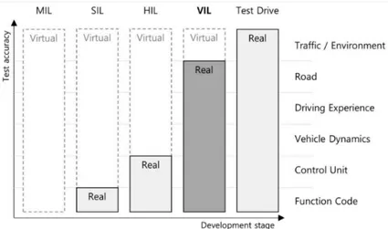
• Model in the loop (MIL) • Software in the loop (SIL) • Hardware in the loop (HIL) • Vehicle in the loop (VIL)

Figure 2.1.2 compares the difference between different modeling methods. MIL is useful for quick development and verification of algorithms by modeling the controllers in the computer system. In SIL all aspects of the vehicle’s physical state and response is modeled by modeling the sensor data and feeding it to the world or environment simulation. The HIL system has some degree of hardware integration for example feeding data from the real-world camera (or any other sensor) into the simulation. Similarly, VIL allows for a more accurate test and assessment by using the vehicle to produce responses to simulated stimuli. VIL is intended for a production-ready vehicle that has perception, control, navigation, and other modules in place.

Figure 2.1.2: Comparison of (see [22]) MIL vs. SIL vs. HIL vs. VIL vs. Test Drive

In this thesis work, only the SIL approach is used to generate test cases and compute its complexity. However, generated scenarios can be used with any of the above methods.

2.1.2

Closed track testing

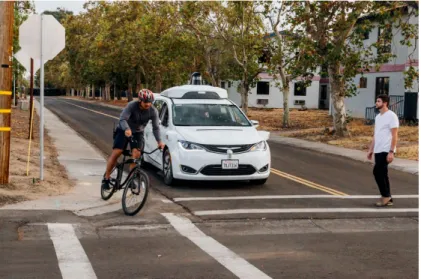
This method is deployed generally after simulation testing to capture those aspects that could not be captured using simulation due to inaccuracy in modeling. Also, it is crucial to test the autonomous agent in a life-like controlled environment to validate the simulation results. This method is used for physical testing of a production-ready vehicle with actual functional software on the target platform. The vehicle is presented with real obstacles and participants. This method

provides a high degree of control that is not possible in real-world testing. However, the method may be extremely costly, for example simulating a crash or accidents involving humans (figure 2.1.3). It may not be scalable to a wide variety of scenarios as it may be difficult and time-consuming to modify the environment for a newer scenario.

Figure 2.1.3: Orchestration of a scenario in closed track testing setup by Waymo

2.1.3

Open road testing

This involves testing the system in the actual public road with reasonable safety measures. This testing method captures the true essence of the environment and provides true feedback on system performance crucial to comply with the safety requirement of government bodies. However, there is no control over the environment and scenarios cannot be repeated with slight variation in the scenario parameters. It is also not possible to reproduce the test with the exact parameters. Open road testing requires at least one human safety driver, who overrides the control to avoid catastrophic events like accidents.

2.2

Traffic scenario description

Modern traffic scenarios are fairly complex. An increasing number of on-road vehicles is only making it more complicated. In order to motivate scientific research in traffic-related topics, it is extremely

important to have a systematic method to define the various scenarios. There have been several attempts to propose a framework to define a traffic scenario. The term scenario is not used consistently in many pieces of literature. Although its usage varies with the field, the core concepts are similar. A traffic scenario contains information regarding the weather condition, road’s physical properties, surrounding information, number of lanes, communication like GPS, the physical state of the dynamic participants, and their functional behaviors. The technical terms defined by Ulbrich et al. [28] are used in our work which is defined as follows:

A scenario describes the temporal development between several scenes in a sequence of scenes. Every scenario starts with an initial scene. Actions & events as well as goals & values may be specified to characterize this temporal development in a scenario. Other than a scene, a scenario spans a certain amount of time. [28]

A traffic scenario describes the scenario in a traffic context. Identification of every possible traffic scene is extremely important for a reliable evaluation of autonomous vehicles. For systematic testing and evaluation, the PEGASUS project report and Menzel et al. [20] break every traffic scenario into three abstraction level:

1. Functional scenario: This is the most abstract level of the scenario. A functional scenario can be described in a consistent linguistic fashion and contains details of the traffic entities and their behavior and interactions. Such a description is particularly useful for risk assessment and hazards analysis during the concept phase. The level of details about the entities and interactions depends on the development phase.

2. Logical scenario: The logical scenario is a more detailed representation of a functional scenario using state-space variables for various entities and their interactions. State-space variables are often defined via a probability distribution. This probability distribution is based on the function design of the vehicle.

3. Concrete scenario: The concrete scenario has the lowest level of abstraction and describes the logical scenario via a combination of concrete value for state-space parameters. These values are sampled from the probability distribution defined in

the logical scenario, by an expert-based approach that depends on Operational Design Domain(ODD) requirements. Finally, the concrete scenario contains enough details so that it can be executed in real-world or simulation.

As per the SAE standard known as J3016, ODD is defined as - the

operating conditions under which a given driving automation system or feature is specifically designed to function, including, but not limited to, environmental, geographical, and time-of-day restrictions, and/or the requisite presence or absence of certain traffic or roadway characteristics.

In the figure 2.2.1, different abstraction levels and details contained in each level can be seen. A lower level of abstraction translates to a more practical scenario that can be used to re-create a scenario in simulation or in the real-world to carry-out the test and evaluation.

Number of scenarios Level of abstraction

Functional scenarios Logical scenarios Concrete scenarios

Figure 2.2.1: Levels of abstraction along the development process in Menzel et al. [20]

2.2.1

Decision variables

As discussed in the previous section, a state-space variable is used to describe the logical scenario. A number of variables describe the complete concrete scenario, see fig 4.1.1. These variables entail the metric, semantic, topological, and categorical information about the scene. For systematic safety and reliability analysis, only a few parameters are studied at a time. Those parameters are called decision variables for a certain logical scenario. All other parameters remain fixed within the ODD. The choice of decision variable may depend on the ODD of the vehicle, the researcher, and the objective of the test being conducted. In general, most of the stationary elements of the scenario are specified by the ODD. Choosing an appropriate decision variable is very crucial for effective and relevant evaluation and can influence the

external validity of the test. All parameters other than decision variables are kept constant. Again, the value of the constant parameter depends on the research objective and researcher. Changing these parameters may require redoing the experiments.

2.2.2

OpenDrive and OpenScenario format

To simulate a scenario, virtual models of static and dynamic objects are required. The modeling requires a high degree of detail and information. Defining a format that contains this information in a structured way is challenging due to the high dimensional nature of the problem. In this thesis, OpenDrive and OpenScenario format is used and was chosen because both of them are open-standard and are reviewed by an expert team consisting of members from BMW, Daimler AG, DLR etc. Detailed information on these formats can be found in Heinz et al. [12].

Figure 2.2.2: Separation of different kind of scenario description contained in OpenDrive and OpenScenario [24]

OpenDrive is an open file format for a logical description of static content like lanes, buildings, signals etc in the scenario. It models the map and road network present in the simulated environment. It uses Extensible Markup Language (XML) to store data. The format is very flexible in the sense that it allows researchers to create templates that can be easily filled with custom data to create different versions of

the scene. It also enables a high degree of specialization in individual projects while maintaining a fair amount of commonalities among many projects. In this work, OpenDrive is used to model the MAN testing facility in Munich, Germany. This map is used to generate critical scenarios in the final phases of the thesis. Using an actual map is useful, as it will allow the investigation of the real-world relevance of results in the future and validate the developed algorithm and architecture. OpenScenario, on the other hand, is an open file format to describe the dynamic content like weather, participant’s maneuver in XML format. The XML consists of goals, trigger conditions, actions, and target values. It provides a catalog of various common behaviors or actions of the entities that can be observed in an urban setting. The entities are dynamic traffic participants like vehicles, cyclists, and pedestrians. The figure 2.2.2 illustrates the data contained in OpenDrive and OpenScenario file format.

2.3

Scenario criticality estimation

The aim of the evaluation is to provide a generic assessment framework of the simulated scenario. A mathematical formulation is used to define what aspects of the scenario should be considered to compute its criticality. The formulation of the criticality model is also an active area of research (see Zhou et al. [33]). Several methods have been proposed that computes the criticality on the basis of safety, functionality, mobility, or rider’s comfort. Formulation often depends on the objective of the experiment and functionality that is being tested. It is difficult to find an analytical solution in the state-space parameter domain due to the high dimensionality and uncertainty of events in an urban setting. Therefore, criticality is often competed by analyzing the simulation data.

The common method to compute the criticality of the scenario is to use metrics like Time to collision (TTC), Time headway (THW), or Responsibility-Sensitive-Safety (RSS). As the focus is on building a generalized architecture for scenario generation, the criticality estimation function is treated as a black box. To investigate the effect of the criticality metric, TTC and THW are used to build architecture. RSS is an interpretable mathematical model for safety assurance. TTC

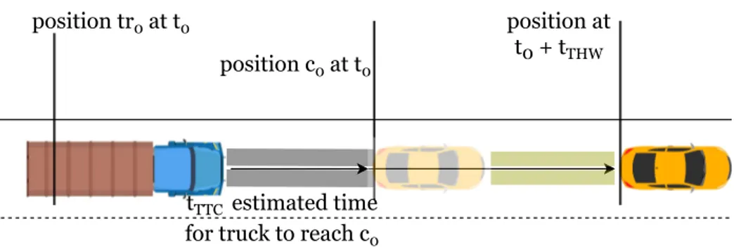
and THW were chosen as these metrics are simple to implement and commonly used by researchers and for traffic control. RSS on the other hand is quite difficult to implement as it does not have a single mathematical form, rather it is a collection of many rules and conditions. A detailed method to build RSS metric can be found in Shalev-Shwartz et al. [25]. The figures 2.3.1 and 2.3.2 illustrate the method to compute TTC and TWH respectively. TTC and THW are used to derive an auxiliary value by using an auxiliary function. The auxiliary function is a mathematical formula defined based on the research objective and is formulated such that its output always lies in [0, 1]. It is one of the important components of the proposed architecture and is discussed in more detail in section 5.3.

positions of vehicles at t0 Estimated motion Vehicles collide at time t₀ + t_TTC

Figure 2.3.1: Illustration to calculate Time to collision based on velocity at time t0 position tr0 at t0 position c0 at t0 position at t₀ + tTHW tTTC  estimated time for truck to reach c0

Figure 2.3.2: Illustration to calculate Time headway i.e. estimated time taken by vehicle to reach the position c0of vehicle in front.

2.4

Bi-cubic spline interpolation

Interpolation is a method to estimate new data based on existing ones. There are several techniques to perform interpolation, for example linear, polynomial, piecewise splines, or gaussian interpolation. Piecewise spline interpolation is being used to construct a probability distribution function from the data computed by simulating the scenarios. Splines are easy to implement and it reduces the oscillations in the interpolation (see [5]) by using a lower degree polynomial function, therefore it was chosen over other methods.

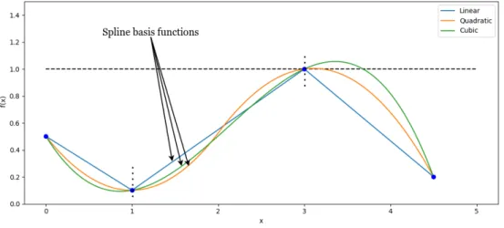
Spline interpolation is a popular method to interpolate a continuous multi-variable mathematical function. Splines use a piecewise polynomial function to parameterize the function. These polynomial functions are called basis functions. Piecewise in the sense that only one basis function is used to interpolate two consecutive data points. The complete function is formed by using a sequence of the basis functions. In figure 2.4.1, polynomials of three different orders are used to interpolate the same points. It can be observed that this method always produces a continuous function and using higher-order polynomials forms nice smooth functions. It should be noted that the estimated interpolation function exactly passes through the data points, therefore they have a zero estimation error.

Figure 2.4.1: Dotted vertical lines are the interval in which one basis function is interpolated. We see that basis function with the order greater than 1 results in over-shooting.

Cubic splines were used as it is recommended to use a basis polynomial function of odd order and it is the lowest odd-order function to ensure the differentiability of the estimated function. The function 2.1 represents the family of a cubic spline basis. The coefficient is determined by imposing continuity and differentiability constraints within the interpolation interval.

si(x) = ai+ bi(x− xi) + ci(x− xi)2+ di(x− xi)3 (2.1)

The final function is simply the summation of all basis functions. More details regarding the splines can be found in the lecture [5].

S(x) =∑

i

si (2.2)

Figure 2.4.2: Cliping the interpolated function within [0, 1]

However, higher-order spline interpolation results in over-shooting. This is problematic as the interpolated function is expected to be in the range [0, 1]. One option can be scaling the interpolated function, but this would result in an estimation error. Therefore, the S(x) is cliped within the range [0, 1] (see 2.4.2).

S’(x) =        0 S ≤ 0 S 0≤ S ≤ 1 1 1≤ S (2.3)

The equation 2.1 can be easily extended to a multivariate problem by using Lagrange-form equations to interpolate a surface. 2-dimensional surface interpolation is called bi-cubic interpolation.

scipy’s interpolate function is used to perform the interpolation which

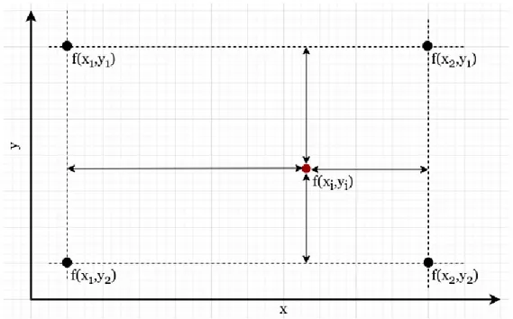
is followed by a clipping step as described in figure 2.4.2. The figure 2.4.3 illustrates a simplified method for surface interpolation.

Figure 2.4.3: Spline interpolation in multi-variate variable space. The value of the function at (x1, y1), (x2, y1), (x2, y2), and (x1, y2) are used to estimate

f (xi, yi)

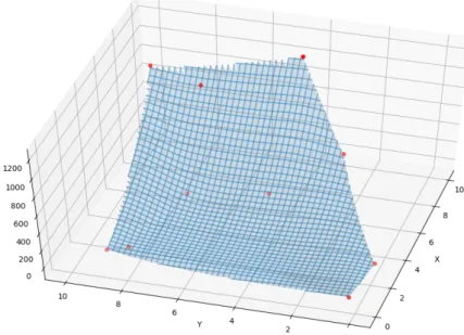
Figure 2.4.4, plots an interpolated surface using the data represented by dots. In this work, those data points are acquired through the auxiliary function. The x and y axis represent the decision variables. It should be noted that interpolation function is only defined for a subset of the domain of decision variables. Therefore, extra care should be taken while generating data that needs to be interpolated.

Figure 2.4.4: Surface interpolation using scipy’s interpolation function in 2-dimension. The region on the top-right is not defined due to lack of data in that region.

Related work

This chapter discusses the relevant work done by other researchers related to the critical scenarios and automatic generation. Computation of the criticality of the scenario is crucial hence it is discussed first, followed by automatic generation methods.

As pointed out earlier, the creation of a testing scenario manually takes a lot of time and is extremely complex. Automation of the test case generation proposes a great value to the autonomous industry. Therefore, there has been a lot of attempts to automate this process. Earlier attempts were limited to finding worst-case scenarios for very specific maneuvers. Jung et al. [14] presents a method to find worst-case scenarios related to J-Turn and Fishhook. Their method used already existing worst-case scenarios to search for a new scenario by optimizing an index function. The existing scenarios were collected from real-world scenarios. LeBanc et al. [19] used naturalistic field operational testing to collect scenario data. In this method, actual vehicles were fitted with a camera and sensor and driven on the public roads to collect real-world driving data. This method provided high-quality real-world data, however, coverage of critical scenarios was very poor and the system often settled with similar and simple scenarios. Also, the data collected represented only regional behavior and did not represent other driving behavior in other parts of the world. Other work by [30] used large-scale naturalistic driving data (NDD) to model the driver model. Through this model, they augmented the NDD using stochastic methods to obtain a more diverse scenario. This was a novel method, however, heavy reliance on NDD imposed a serious limitation

on the scalability of the approach. Althoff et al. [1] developed a fully automatic method to increase the criticality of several uncritical scenarios by optimizing the drivable area of the ego vehicle using quadratic programming. In this method,the original position of the ego vehicle was changed such that the solution space of the correct driving action shrinks, therefore imposing a strict penalty on the vehicle under test. While the algorithm does find a critical scenario, it does not guarantee that the searched scenario will be the most critical one. In [17], the author extended their work in [1] to use evolutionary algorithms to increase the criticality. The work, however, still requires a real-world initial scenario as input to search for a nearby critical scenario. Most methods rely heavily on NDD to generate a new scenario. The inherent problem with this approach is that the proportion of dangerous situations is relatively less as these are rare events. For example, in the US an average driver has to drive 1.3 million kilometers [16] to report an injury. Zhao et al. [32] and [21] reduced the dependency on the accident rate by using a relevance metric for a specific logical scenario. The relevance is calculated by computing the occurrence of a particular maneuver in the real-world by analyzing the NDD. The paper also introduced an accelerated method to deduce the complexity of lane change behavior. The presented method is at least 2000 times faster than NDD simulation approaches.

To create a critical scenario, the criticality of the scenario must be modeled. Mathematically computing the criticality of scenarios has a two-fold advantage - 1) it can be used to identify more critical test scenarios, 2) it can be used to benchmark a driving agent before testing it in the real world. Modeling the criticality of the scenario is extremely challenging and it is still an active area of research. J. Zhou et al. [33] used a test case catalog to reduce the dimensionality of the scenario. Reducing dimensionality improves the assessment of the scenarios which eases the formulation of a mathematical model to compute the criticality of the scenario. Junietz et al. [15] proposed a method to compute complexity based on the parameters of model predictive control trajectory optimization.

[21] developed an architecture to perform end-to-end testing of the autonomous vehicle, even the stack that includes a deep learning perception and control models. They used standard traffic behavior to model the probability of rare events. The algorithm is agnostic to the

complexity computation metric and treats it as a black box. Calculating the probability of a critical scenario is a much better approach than finding a bunch of scenarios as there is no limit to the number of critical scenarios that can be generated using the distribution. This is particularly important for large-scale testing of an autonomous vehicle in a simulated environment. S. Feng et al. [9] provided a general framework for test scenario generation with different operational design domains, autonomous agents, and complexity metrics. The criticality of every scenario was measured by combining maneuver challenge and exposure frequency. Exposure frequency is the scenario importance metric of the scenario, derived from the NDD. An auxiliary value function is formulated based on the critical value of each scenario, which is used to search for the critical scenarios using a reinforcement learning-based approach. However, this technique resulted in a fewer number of critical scenarios for testing and evaluation of the autonomous agent. In this work, the framework and complexity computation method in [9], and in [8], is combined to compute a probability distribution as described in [21].

Evaluation

requirements descriptionScenario Metricdesign generationLibrary evaluationVehicle's

Evaluation results Design

variables Performanceindex Generatedlibrary

System modeling

This chapter elaborates on modeling the simulation architecture. The objective scenario is discussed first, followed by the map and the car model. The simulation requires an autonomous driving agent, which is discussed later in this chapter. It is required that the architecture is modular, robust, and scalable therefore the important functional blocks are splitted into carefully planned modules. The algorithmic parts of the architecture are treated as a black box so that the functionality of the architecture is not influenced by the optimisation and criticality metric implementation.. The important parts that can influence the quality of output are critical value computation, auxiliary value, optimization, and interpolation function. Hence, they are separated into different functions in the code. This ensures that changes in any of the mentioned parts will have a minimal negative effect on the functioning of the architecture. Also, trusted open-source libraries and packages are used to reduce the failure due to faulty implementation and also benefit from the open-source community.

4.1

Objective Driving Scenario

Real-world traffic scenarios are extremely complex and high-dimensional, which presents a great challenge to model the scenario accurately and study its behavior. Research has been done to reduce the dimensionality of the problem (see [33]). However, for the sake of simplicity, a simple maneuver is considered to start with as the focus is on building the architecture. A simple cut-in maneuver is chosen

as an objective logical scenario. This kind of maneuver is an extremely common sight in urban traffic which means that a huge amount of real-world data is already available for this scenario. This data can provide valuable insights that can motivate the choice of decision variables. In figure 4.1.1, various possible parameters are shown that can influence the criticality of the scenario. In a cut-in scenario, the ego vehicle’s path is interrupted by another vehicle in the adjacent lane as it invades the ego vehicle’s lane. This vehicle is called a background vehicle.

Figure 4.1.1: Logical scenario used in this thesis. It highlights a subset of variables that affects the criticality of scenario

To be able to execute the scenario in the simulation, every aspect of the scenario must be clearly defined. Defining a scenario is a three-step process. It starts by defining the operational design domain using a functional scenario. In figure 4.1.2, the desired setting and behavior are indicated in plain English. In the next step, all the important parameters are listed(see figure 4.1.3a) and their probability distribution is defined. The probability distribution can be expert-based or can be derived from

the traffic data. The weather conditions, road friction, time of the day, vehicle type, etc is also considered and their values are decided. They are not listed in the logical scenario diagram 4.1.3a for the sake of simplicity as they are not very important for our experiment. All the experiments are performed at noontime in the simulation. The effect of daylight is not part of the study in this work. But logically, daylight should affect the criticality of the scenario. Similarly, cloud conditions and road friction were also fixed throughout the experiment to simplify the problem. The exact settings are found in the OpenScenario logical file attached in the appendix A. The attached file is a template with placeholders for the

decision variables 2.2.1 and derived parameters.

Derived variables are the parameters that are not part of the study,

but it must be adjusted for every concrete scenario so that the exact scene defined by the decision variables can be orchestrated in the simulation.

Cut-in functional scenario

Static object 

Road has layout two lanes. Road has geometry straight. Dynamic object 

Truck has position on left lane. right lane. has position on Car in front of the truck. changes lane Car

Figure 4.1.2: A functional scenario description for the scenario used in the thesis

The concrete scenario is created by sampling the parameters from their respective probability distribution in 4.1.1. The solid line in figure 4.1.3b shows the exact value of every parameter. The dotted lines show the different values for different scenarios that are executed in the simulation. It should be noted that the values of several parameters are fixed and even a simple scenario like Cut-in can have a large number of parameters that influence the criticality of the scenario. Therefore the effect of only two variables is studied i.e effect of range (R) and range rate ( ˙R)on the criticality. Apart from the decision variables and

the initial position of the background variable, all other parameters are kept constant. R and ˙Ris the relative longitudinal distance and velocity between the background vehicle and ego vehicle respectively at the time of the cut-in. To ensure that the lane change occurs, both the vehicles are explicitly controlled until the lane change event is triggered by the

scenario executor, after which the autonomous agent takes control of

the ego vehicle.

Cut-in logical scenario Static object  Left lane: width Dynamic object  Truck: long. vel. p 0m 100m Right lane: width p 3m 5m p 3m 5m p 0km/hr 60km/hr Truck: long. pos. p 0m 1000m car: long. vel. p 0km/hr 60km/hr car: long. pos. p 0m 1000m Cut-in rel. dist. p 0m 100m Lane-change dist.

(a) The logical scenario describes the important parameter and its

probability distribution.

The figure does not contain daylight, cloud, sun position, and road friction configuration details. Cut-in concrete scenario Static object  Left lane: width Dynamic object  Truck: long. vel. p 0m 100m Right lane: width p 3m 5m p 3m 5m p 0km/hr 60km/hr Truck: long. pos. p 0m 1000m car: long. vel. p 0km/hr 60km/hr car: long. pos. p 0m 1000m Cut-in rel. dist. p 0m 100m Lane-change dist.

(b) The concrete scenario describes

exact values

of the parameters, sampled from the probability distribution. The dotted lines show different configurations of parameters.

Figure 4.1.3: Formulation of the logical and concrete scenario

To sum it up, the objective logical scenario is simplified to have the following decision variables:

1. The relative velocity of the background vehicle with respect to ego vehicle ˙R.

2. Relative distance between the ego and background vehicles when lane change is triggered R.

4.2

Initial set-up of the scenario

The exact value of the decision variables is defined in the OpenScenario file. The scenario executor uses these values as the target and tries to match them in the simulation. In practice, however, it is difficult to achieve both the targets simultaneously. Therefore, the initial position of the background vehicle is set such that the vehicle always matches the targets at simulation time t = 6sec. Therefore, cut-in maneuver always starts at 6 seconds for all simulated scenarios. This is achieved by adjusting the initial position of the background vehicle. The initial velocity of the background vehicle is calculated using equation 4.1. The initial position on the background vehicle is computed using the equation 4.2. Lcm is the sum of the distance of the back of the

background vehicle and front of the ego vehicle from their respective center of mass. The figure 4.2.2 graphically illustrates the calculation of

Lcm. It is evident from the figure that the value of Lcmwill be different

for every pair of ego and background vehicles. The implemented architecture provides a single configuration file to define such constants. Hence, when the value of Lcm is updated in the configuration file, the

initial position of the background vehicle must be re-calculated.

vbackground= vego + ˙R (4.1)

where ˙Ris the desired relative velocity.

pbackground_initial = pego_initial− ˙R ∗ 6 + R + Lcm (4.2)

[R, ˙R] is the desired decision variable for a concrete scenario. The table 4.2.1 list all the variables used in this work, along with their meanings.

Save to XML _OpenScenarioConvert to

R R Other variables Concrete Scenario .

Figure 4.2.1: Parser to generate concrete OpenScenario file from decision variables. Decision variables are saved in XML file along with the derived parameters.

CM

CM

L

l

l

Figure 4.2.2: Lcmis different for different pair of vehicles.

Variables Explanation

θ Pre-determined parameters for testing scenario

pego Position of ego vehicle

vego Velocity of ego vehicle

pbackground Position of background vehicle

vbackground Velocity of background vehicle

R, ˙R Relative distance and velocity between the ego and background vehicle at the time of lane change

x Decision variables for the testing scenarios, [R, ˙R] q(x) Complexity metric

r(x) relevance metric

wi Weight parameter

J (x) Auxiliary objective function

J′(x) Interpolated auxiliary objective function

lego Distance between front of ego vehicle and its center

lbackground Distance between back of background vehicle and its center

Lcm lego+ lbackground

si Set of sampled scenarios in ithstep

Si Union of all sampled scenarios till ithstep;∪ij=0sj

Table 4.2.1: List of the variables and their meaning

The values of the decision variables are stored in an XML file (see appendix B). These values are generated automatically by the algorithm.

A parser is used to combine these values and the logical scenario template to generate a concrete scenario file. It is possible to produce the concrete scenario directly from the generated decision variable, but an intermediate step to store the data in XML was introduced. XML is a popular standard supported by the majority of the systems, therefore storing the generated data in XML will allow possible integration with other platforms in the future. Also, this architecture will allow easier upgrades to newer versions of OpenScenario. Figure 4.2.1 outlines the module that produces a concrete scenario from the generated decision variable.

4.3

Simulation environment

The simulation environment models the real-world physics and behavior of various participants. The external validity of any experiment carried out in the simulation environment is heavily influenced by the modeling accuracy and experiment’s objective. Although the cut-in scenario experiment performed cut-in this thesis does not necessarily require a very detailed simulation as it does not use any visual feedback from the environment to compute the criticality or to control the ego vehicle. But the architecture was also expected to test the visual or lidar based system in future therefore, a detailed modeling of the environment was required. Apart from that, the simulation environment should also support the OpenScenario and OpenDrive format.

There exists several simulation software that focus on autonomous driving for example Carsim, CARLA, Apollo etc. CARLA [6] (version 0.9.10) simulation platform was strategically chosen as it is open source and has active support from the community. It also supports OpenDrive format to layout road networks. The CARLA simulator uses Unreal (more detail at [7]) game engine to render 3D graphics and has a python binding to allow development in Python.

CARLA offers a high degree of control over the simulation and behavior of the participants. It provides an official package called

ScenarioRunner (version 0.9.6) that can orchestrate a given scenario

and perform common maneuvers like a lane change, follow a lead vehicle, etc. It partially supports OpenScenario format and is under a

rapid development phase, which imposes some limits to the modeling of the scenario. Because of these limitations, it becomes difficult to achieve the desired decision variables in the simulations. It is extremely important to minimize the error in desired decision variable values for the computed auxiliary values to be relevant. The ScenarioRunner runner converts the maneuvers specified in the OpenScenario file into a behavior tree to orchestrate different actions or maneuver sequentially or in parallel.

0.0 2.5 5.0 7.5 10.0 12.5 15.0 17.5 20.0 Simulation time (sec)

0 20 40 60 80 100 Longitudinal distance (m)

p

p

R

p

p

L

Figure 4.3.1: Orchestration of a single traffic scenario. Nature of pego

illustrates how the ego vehicle reacts to avoid the collision.

The initial position of the background vehicle is carefully calculated in section 4.2 to meet the trigger conditions. But during simulation, it was found that the error in achieving [R, ˙R]was high due to noise introduced by the simulation environment. Therefore, noise was removed explicitly for the first 6 seconds of the simulation. Figure 4.3.1 and 6.2.1a plots the maneuver and accuracy of the simulation. For the illustrated scenario the error is in order of 0.3m which is less than 1% of the maximum R i.e 40m. Appropriate error analysis of the scenario can be a separate research topic in itself. Any tests to explore the exact cause of this error were not performed, but modeling and numerical error can be a possible cause. To achieve this extra control over the simulation, a custom scenario executor was developed by inheriting the CARLA’s

ScenarioRunner 4.3.2, referred to as simply scenario runner further in

the text. This custom scenario runner contains functionality that solves the issues discussed above.

To perform the experiments, several (generally >10) scenarios are provided at once. Therefore, the system should be reliable enough to safely execute all the scenarios by handling all possible scenarios. However, it is extremely difficult to imagine all scenarios therefore a simple error handling was implemented initially that just terminated the simulation on encountering any run-time error. But this solution resulted in the loss of simulation progress. Therefore, a stop and resume feature was added to simulate only the un-simulated scenarios when it is restarted. In figure 4.3.2, the module to execute the scenarios and data collection is illustrated. The scenarios are provided in OpenScenario format produced by 4.2 step. The scenario runner also creates a video of the simulation to visually analyze the quality and validity of the scenarios. The data simulation data is stored in a CSV file for cross-platform support. The data for every scenario and iteration is organized in a well-defined folder structure (see appendix C) which is automatically generated by the architecture.

Custom ScenarioRunner wrapper Carla ScenarioRunner List of concrete  scenarios Carla Server Data acquisition Simulation progress Initial set-up

Figure 4.3.2: Architecture to accurately simulate a list of concrete scenarios. The concrete scenarios are provided in OpenScenario format.

The CARLA simulation environment can be configured to be used in

synchronous and asynchronous mode. Using the synchronous mode

configuration, the simulation time-step and real-world timing between the simulation frames can be controlled explicitly. Since there is no human input required during the simulation, the simulation can be executed at super-human speed to save time. Hence we use synchronous

mode in this work. More details about the mode and its usage can be found in the documentation [4].

4.4

Vehicle modeling and driving agent

Vehicle modeling has the following two aspects: physics of the model and rendering. Both are defined in the Unreal engine while building the model. The model was provided by MAN Trucks and Buses. More details on modeling can be found in the CARLA documentation [3].

The behavior of all participants is defined in the concrete scenario, except for the ego vehicles. The ego vehicle, by definition, is supposed to react depending on to the perceived environment. Therefore, an agent is needed to autonomously control the ego vehicle. Generally, this agent would be the driving agent that needs to be tested. Every agent behaves differently under similar situations, therefore the generation of the critical scenario is actually influenced by the agent’s behavior. Ideally, critical scenarios should be independent of autonomous agents so the dependency on the autonomous agent’s feature is reduced by using a surrogate model agent.

The surrogate model always behaves according to the traffic guidelines or behaves according to the defined rules. CARLA autopilot agents are used as the surrogate. CARLA autopilot cheats the simulation environment as it has complete information about its state and surrounding, for example, road network, velocity, and position of all traffic participants, etc. The autopilot uses this information to make driving decisions. In the real world, it is never possible to have access to such detailed information. The controllers required to smoothly control the vehicle are already built inside the agent and CARLA provides high-level APIs to easily use the autopilot.

Using autopilot has the following advantages, it reduces development overload and faulty implementation and it can be conveniently replaced with an actual agent to perform testing and benchmarking.

4.5

Overall architecture

The output from the simulation architecture is used by the optimization module to generate new scenarios that are more critical thus, closing the loop and forming the complete architecture that computes a probability distribution of critical scenarios over the decision variable. The architecture requires an initial set of scenarios to begin with, after which the optimization loop takes over.

To improve the relevance of the scenario to the real world, the idea to use exposure frequency (see [9] and [8]) was discussed. The exposure frequency can be calculated from NDD. The architecture has a placeholder function to integrate the exposure, but it was not integrated due to lack of time to acquire and integrate NDD. Figure 4.5.1 highlights the different modules developed to build the architecture.

Parser Custom scenario runner Initial decision variables(X Initial decision variables(X Set of initial decision variables(x) Initial decision variables(X Initial decision variables(XSet of OpenScenario Logical scenario Spatial frame by frame data Event based data Video data Criticality function Naturalistic Drive Data (NDD) Auxiliary function Probability distribution Re-sampling START OUTPUT N iteration

Figure 4.5.1: Overall architecture to generate the probability distribution of critical scenario

The completed architecture was integrated into the bigger project that contains other modules related to autonomous driving, for example, localization, perception, path planning, and visualization functionality. Tests were written to ensure the error-free execution of the module against the changes in other modules of the larger project.

Proposed method

This chapter discusses two mathematical methods to compute the criticality of the scenario, followed by the formulation of the auxiliary function. Then initialization and re-sampling of new scenarios are discussed. In the end, testing and library generation is discussed.

5.1

Criticality metrics formulation

The criticality metric operationalizes the scenarios to produce a value between [0, 1]. To compute the criticality for a single scenario, the state of the relevant participant is considered at every time frame. If the state at a particular instance of time in the scenario is critical, the whole scenario is considered as critical. It is logical to think that the events in the traffic that can cause damage to humans or other traffic participants are critical. Therefore, certain events are looked for during the simulation to categorize them as critical. Klischat et al. [17] focuses on collision to compute the criticality but identifying the states that may lead to collision in future is also important.

Given a state, the NDD can be used to search for the closest scenarios that lead to a collision and then use the closeness to derive the criticality. In theory, this approach may provide a very reliable estimate of criticality as it uses real world data to build a statistical model of the criticality. But this method requires a huge amount of road accident data. Given the fact that accidents are very rare events [16], it will be extremely difficult to build such a model that could provide any reliable

insight. But the concept can be utilised in a simulated set-up. In this work, two techniques are investigated to compute the criticality.

Apart from the proposed metric, another metric like Responsibility-Sensitive Safety(RSS) [25] was explored. The RSS is a powerful metric as it contains the guidelines for safety, but it is very difficult to implement, therefore RSS was not implemented in this work to limit the focus on architecture development. Use of RSS presents an interesting scope for future work. It should be understood that the metric formulation can vary a lot depending on the logical scenario and its decision variables.

5.1.1

Time to collision

TTC is an event based metric that relies on possible future collisions while performing the maneuver. Feng et al. [10] shows minimum time to collision is a good metric to estimate the criticality at any given point in time for a cut-in scenario. Considering the configuration in figure 2.3.1, TTC is calculated by predicting the path of the vehicle using the position and velocity at the current time to. Then a collision point is

checked for at a future time to + tT T C. If there is a collision, then

TTC = tT T C otherwise it is not defined as defined by equation 5.1. The

prediction is made only for the next 10 seconds as the calculation is expensive and longer time to collision are not critical. If there is no collision within 10 second, then tto

T T C = 10is assumed.

tto T T C =

{

−pbackground−pego−Lcm

vbackground−vego (vbackground− vego) < 0

∞ otherwise (5.1)

TTC is calculated for every time frame, and only the worst TTC throughout the simulation is considered. The worst TTC is the minimum

tto

T T C observed during a simulation. T T Cmin =min

t (t t

T T C) (5.2)

The value of T T Cmin may not necessarily lie between [0,1], therefore

a transformation function (eq. 5.3) is used to squeeze the range. The function qT T C is the measure of criticality of a scenario with decision

corresponds to non-critical scenarios, while any value in between means there is a possibility of collision.

qT T C(x) = e−T T Cmin (5.3)

5.1.2

Time headway

Another widely used metric used to measure urban traffic flow is time headway. As proved in [2], THW is used by the driver to monitor the car in front on the highway. Since the logical scenario is very similar to highway driving, THW seems very promising. Similar to the minimum TTC, we only consider the worst THW throughout the scenario. As illustrated in the figure 2.3.2, THW at any time t = to is the time taken

by a vehicle to arrive at the position of the leading vehicle at time t = to.

Again, the prediction is made upto 10 seconds in the future, if the vehicle is not able to reach the position pego within 10 seconds,then ttT HWo = 10.

The minimum time headway can be calculated as in the equation 5.5 is assumed. The range is squeezed between [0,1] using the equation 5.6. tto T HW = pbackground− pego− Lcm vego (5.4) T HWmin =min t (t t T HW) (5.5) qT HW(x) = e−T HWmin _(5.6)

5.2

Importance metric

It is important to consider scenarios that are more common in real-world as the agent must be able to handle the common scenarios as well. The importance of a generated scenario can be calculated based on the exposure frequency. More details on calculation of exposure frequency are given in [8]. As mentioned in 4.5, the importance metric was not actually used in this work, however a placeholder function has been created for future implementation and extension of the work. The importance metric is denoted by r(x) with range of [0,1]

5.3

Auxiliary function

Auxiliary function combines criticality metric q(x) and importance metric r(x) through a weighted sum (see eq. 5.7). The weights are chosen by an expert based on optimisation objectives. For example, if the objective is to generate more on the common scenario rather than critical ones, then weight wo should be reduced.

J (x) = q(x)w0+ (1− w0)r(x) (5.7)

where w0 < 1

The equation for auxiliary function J(x) can be generalized to incorporate multiple functions to calculate criticality. The equation 5.8 is the generalized equation with n critical value functions. It must be noted that summation of all weights is always 1.

J (x) = Σn_i=0−1q(x)wi+ wnr(x) (5.8)

where Σn

i=0wi= 1

5.4

Optimization of scenario

5.4.1

Initialization

The optimization requires an initial set of scenarios to begin with. The initial set is sampled from a uniform distribution over the decision variables [R, ˙R]. First a naive random sampling was implemented, however it was found that the sampled scenarios were not evenly distributed (see figure 5.4.1) which led to unequal representation of decision variables while computing the probability distribution. The green and orange patch highlights the high and low density regions respectively. To improve the quality of initial samples, stratified random sampling was used. In Yunming et al. [31], this method was used for a better representation of each feature in high dimensional feature space. The conclusions derived from their work can also be applied to this work as it faces the same problem.

To perform random sampling, the decision variable domain space was divided into equal regions, called stratum and one sample was selected

from each region at random. This technique is called stratified random sample with one random element per stratum. In the figure 5.4.2, it can be observed that the scenarios are distributed uniformly across the decision variables.

Figure 5.4.1: Scenarios are not distributed evenly, Green patch highlights the high density region and orange highlights the low density.

15 10 5 0 5 10 15 20

Tigger relative Velocity 0.00 2.86 5.71 8.57 11.43 14.29 17.14 20.00 Trigger Distance

Figure 5.4.2: Stratified random sample with one random element per stratum produces a uniform distribution

5.4.2

Auxiliary function estimate and re-sampling

Data acquired from simulation of the scenario is used to compute the auxiliary values 5.3, which is interpolated using the bi-cubic spline basis 2.4 function. In the equation 5.9, the estimated auxiliary function J’(x) is a function of decision variables x. The interpolation produces a surface with range [0,1], as shown in figure 5.4.3. The

red and green color corresponds to critical and non-critical scenarios respectively.

J’(x) = Bi− CubicSpline(x|J(x0), J (x1),…, J(xn))∀xn∈ Si (5.9)

(a) Auxiliary value of the sampled scenario

(b) Interpolated function computed using the values in 5.4.3a

Figure 5.4.3: Interpolation of computed auxiliary value of sampled scenarios

The probability function is computed by normalising the J’(x) estimate using the equation 5.10. However, to re-sample new scenarios, the

scaling is not required as scaling does not affect the likelihood of scenarios.

p(x) = ∫ J’(x)

J’(x)dx (5.10)

The estimation of J’(x) is based on the scenarios generated in all the optimisation steps because criticality of the scenario is independent of the current estimate of the auxiliary function J’(x). List of all scenarios

Sigenerated till iteration i can be computed using equation 5.11. The sk

is the list of scenarios resampled at iteration k and s0 is the list of initial

scenarios.

Si =

i∪−1 k=0

sk (5.11)

The re-sampling of scenario skat iteration k is done using Monte-carlo

sampling [29] based on the p.d.f p(x) 5.10. Number of samples is defined in the configuration file.

5.4.3

Stopping criteria

Since the focus is on getting an estimate of the probability distribution of the critical scenarios, it is logical to define the stopping criteria based on the p(x) or J’(x). It is clear that the algorithm has converged when J’(x) becomes stable i.e there is very little change in J’(x) with subsequent iterations. The absolute difference in consecutive J’k−1(x)and J’k(x)is

calculated and the optimisation loop is terminated 5.12 if the difference is less than a small ϵ. The value of ϵ is chosen by experimentation. The algorithm can also be terminated manually.

5.5

Testing and Library generation

Computed probability distribution of critical

scenario

N sampled

scenario OpenScenario Parser Library of criticalscenario

Figure 5.5.1: Proposed method to sample a set of critical scenarios from computed distribution for the AD testing

After the algorithm converges, it produces J’(x) and p(x) as the output.

J’(x) can be used to sample the desired number scenario for the testing. In Feng et al. [8], authors used a similar architecture to search the critical scenarios. Their method was limited to generating only a few critical scenarios that must be decided before performing the search. The presented algorithm computes the distribution instead. Therefore, the distribution can be used to generate an arbitrary number of critical scenarios that can be decided at the time of testing. Figure 5.5.1 describes the software architecture for library generation.

The CARLA autopilot should be replaced with the autonomous agent that needs testing. The following architecture 5.5.2 was proposed to perform testing and evaluation. However, the architecture was not tested with any other agent due to unavailability of a different agent. The evaluator module in the architecture can be replaced with a custom evaluator function depending on the evaluation objectives.

Generated Library Autonomous agent Scenario runner Evaluation

Figure 5.5.2: An illustration of proposed method for an autonomous agent evaluation

Experimentation and results

In this chapter, different experiments and their analysis are described. The experiments test the robustness, accuracy, and analyze the choice of criticality function. The computed probability distribution and convergence of TTC and THW metrics are compared.

6.1

Robustness

and

relevance

of

the

architecture

As discussed in the section 4.3, the car model and the map used in during the development of the architecture were taken from CARLA’s library to remove the possibility of error due to modeling errors. But those models are not relevant to MAN Trucks and Buses’ objectives. The objective of the project was to build the architecture to test the autonomous driving capabilities of its trucks. The company also has a testing ground in Munich, Germany. Therefore, using their corresponding model to perform the experiment would be more advantageous as the result can be tested in the real world to confirm its validity. The models were swapped with a MAN’s production truck and a map of T2 track testing facility. The driving challenge was kept the same so that the robustness of the architecture could be tested with respect to map and vehicle model.

The scenario needed to be adapted according to a different road network in the new map. The T2 map had just two lanes and orientation of the lanes were also different. The new scenario was successfully executed

with a slight modification in the code. The cause of modification was related to differences in the modeling of the road network and the vehicle. The vehicle had a different dimension and center of mass settings. These parameters were initially hardcoded in the architecture, therefore it needed some adjustment. Finally those parameters were made configurable with the help of a configuration file. Figure 6.1.1 shows a screenshot of the scenario simulation with the new models. It should be noted that the scope of this work is limited to simulation and no real world experiments were performed to validate the results but it will be interesting to test this in future works.

Figure 6.1.1: The map and truck model used for the rest of the experiments are digital models of the actual test track and truck. The red dots mark the historical position of the vehicles. The generated scenario translates to a real world scenario as the map and trucks represent real objects.

6.2

Simulation accuracy

It is very difficult to orchestrate a scenario in simulation exactly as intended. As mentioned in section 4.3, the architecture has features that tries to minimise the error during the simulation. Figure 6.2.1 plots the

error in R and ˙R as the number of simulated scenarios is increased. A major part of the scenario is controlled by the CARLA’s ScenarioRunner, hence there are a lot of black boxes for us that may result in error.

0 100 200 300 400 500 600 700 800 Number of simulations 1.00 0.75 0.50 0.25 0.00 0.25 0.50 0.75 1.00 Error (m) (a) R 0 100 200 300 400 500 600 700 800 Number of simulations 0.20 0.15 0.10 0.05 0.00 0.05 0.10 0.15 0.20 Error (m/sec) (b) ˙R

Figure 6.2.1: Error in simulated and desired decision variables

From the plot, it can be observed that the mean error stabilizes to a constant value. The co-variance of the error is high and constant which might be the result of systematic noise introduced by the simulation environment. We also note that the mean error in velocity has an offset and is consistent. In the architecture we explicitly specify the velocity of both vehicles, therefore error might be the result of the motion modeling and the controller used in CARLA. Another possible source of error may be the ScenarioRunner itself as it is still under development and