Analysis of vapor barrier experiments to evaluate their effectiveness as a means to mitigate HF concentrations: final report

~

4. 5 "Model Studies of LNG Vapor Cloud Dispersion with Water Spray Curtains," Meroney et al., 1983, '1984, and Heskestad et al., 1985 Experiment Configuration:

A series of model tests were funded by Factory Mutual Research, Inc. and the Gas Research Institute to evaluate the ability of water spray curtains to reduce concentrations around an LNG spill below flammability limits. Water sprays are not expected to remove natural gas ·from LNG spill clouds. The objective of the water spray is to entrain air and dilute the cloud below the flammability limit. Thus, these experiments do not simulate the potential for HF reduction due to water-spray induced deposition. Since the desire was to determine concentration reductions immediately downwind of the spray curtain measurements were only made out to equivalent distance~ of 390 m from the release point. One series of measurements were also made to validate the simulation methodology using field data from the C02/water spray tests performed by Moodie et al.

(1981) at a scale ratio of 1:28.9. Carbon dioxide was released from a point source upwind of an array of water spray nozzles (Figure 4.5-1). Both ground level and vertical profiles of concentration were taken.

Most of the measurements were made over a 1:100 scale model of a 60 m x 60 m bunded spill area (Figure 4.5-2). Many different arrangements of water spray release points, nozzle orientations,· nozzle sizes were considered (Figure 4.5-3). Vapor barrier fences varied in height from 4 to 16 m. A small (S), medium (M), and large (L) tank were situated within

the bunded area during some tests (Figure 4.5-4). Tank diameters ranged from 22 to 36 m, and tank heights ranged from 23 to 28 m. LNG boiloff rate (3000 to 21,400 cubic meters/sec gas) and wind speed (1.7 to 8 m/sec) were also varied.

These data have been extensively examined previously to evaluate the optimum performance of a water spray curtain (Heskestad et al., 1983) or to calibrate a numerical dispersion model (Meroney and Neff, 1985.) This review will focus on the various vertical profiles measured, the effects of discharge on barrier influence on the dense gas cloud, and the relative reductions in peak concentration seen downwind of various size tanks. Results of Comparison:

Consideration of data from Meroney, Neff and Heskestad (1984) showed that peak concentrations were reduced to values of 0.21 some 5 m downwind of the water curtains modeled, then the ratio began to rise at farther distances downwind (Figure 4. 5-5). A vertical concentration profile measured along the centerline at a distance of 18.3 m reveals that the water spray re-distributed the mass of the plume upward and reduced peak concentrations by 75 % (Figure 4.5-6).

A water spray system was found to reduce peak centerline concentration ratios to 0.1; however, a tank placed within the spill area tended to lift the gas into the upper separation cavity downwind of the tank. Thus, aerodynamic turbulence pre-mixed the gas to significant

heights, even before the cloud reached the water spray curtain. Figure

4.5-7 shows that concentration ratios with the tanks present increase from

0.2 to 0.8.

Figures 4.5-8 to 4.5-11 display centerline vertical concentration profiles with and without a water spray activated for the conditions of bund alone, small tank, mediwn tank, and large tank. Without water spray or tank the dense plwne remains below a height_ of 10 m, but the tanks mix the gas up to a height of 20 or 30 m. The water spray curtain then distributes the cloud to heights above 30 m.

Increased water flow through the spray nozzles tends to increase the entrainment velocity, w0 • Figure 4. 5-12 summarizes the net effect of increasing water discharge for all ·data disregarding nozzle or spray arrangement. Water flow rate appears to dominate dilution; whereas nozzle number, size and orientation produce only second order effects.

The increased entrainment associated with larger water discharge rates leads to deeper, well-mixed plumes 1downwind of the spray curtain (Figures 4.5-13 and 4.5-14).

Conclusions:

Water spray curtains were found to dilute dense gas clouds by factors ranging from 3 to 50. Large tanks and fences result in increased mechanical mixing which dilutes the dense gas before it reaches the water curtain; hence, effectiveness of the curtain decreases. Nonetheless, the combined effect of tank and water spray curtain on air entrainment was more than the enhanced mixing induced by either object alone. Water spray curtains mix dense gas clouds to considerable heights as a result of their entrainment of air into the gas cloud. Water spray curtain effectiveness increases directly with the rate water is discharged through the curtain.

1 eo .4 T5e(t.9) 0.6 2• 0.6 T37e (1.3) 0.7 3• 0.6 T4

e

(0.9) 0.1 TBe (1.2) 0 .9 Tl7 (1.6) 1.2

Fig. 4.5-1 Experimental Configuration and Measurement Grid, Health and Safety Executive C02/Water Spray Trial No. 46

010

~

011 [ o& 01 oa 09 012-1 ~ 0

" :: gJQry

l

~:~

7

'_~

... ! __ 0 ...

~-

34

g;~

___

_.,o._3~-

....

L

022---. 035 038 045 023 T 60 024 025 026 027 028 90 120 60 120

o •Ground Level" (0.5 above Ground)

• •Ground Level" Plus Elevations 3.5, 7.5, 15, 30

Fig. 4.5-2 Experimental Configuration and Measurement Grid, Generic Bunded Spill Area

• •

[]

Con! l9urallo11 A

El

Conl•gurol•on G Fig. 4.5-3

.

[]:

__..._

.

• C4nf>gut0h0fl •

~J

_{• • •} Conf,gu•ol ion H ••••••••••••• •

•

.[].

• _• • _• •

•

.

• _•

--

.

•

_• • • •

•

•

_{•••••••••••••} • Conli9u•Olloft C • • •

•

. G.

• _-+-

•

• • • • eo~r.guror.on 1

[]

·:

• • • Conll;uralloft D

[]:

Conli;urotlol\ J

E]:

Conligu1ation E •

•

•

•

•

.[].

.

.

.

• -+- • • • • • • • • • • Conf,g u r~t . on ·I(

Water Spray Configurations for Generic Bunded Spill Area

64 • • • • • •

~r

·Conli<;1uror1on F

• ••••••

.[]

•

.

.

.

.

• • -+-. • •

_•

• _• • • Conl iguroti·on L

r

!

·

!

!

I

23J em

!

l23L

I

j

:

If

28.3cm

+1

I ·:

_, 1 ₁

J~

_8cm I _t I ₁ 16.cm

_{_Ll}

I

I•

60 cm

~

I•

60 cm

~

I•

60 cm

~

Small Medium Lorge

Fig. 4.5-4 Tank and Fence Configurations for Generic Bunded Spill Area

65

....

0 ~ u ... ::i: u 1 0 . 8 0 . 6 0. 4 0 . 2 0 0 !Curtain Position

I

Point Source of co zit ground level I

I

I

~p:a~ :~::~e:tp~~n:ed

dovnward vertically

I

I 20 nozzles spaced equally over 29 m

Nozzles vere an Angus Fyrhed 14 mm at 46 kPa

10 20

Distance (m)

30

Fig. 4;5-5 Peak Concentration Ratio vs Downwind Distance, HSE Trial No. 46

4

Point Source of

co

zit ground level

u

=

1 mtsec at 10 m

3 Spray nozzles pointed vertically

downward

20 nozzles spaced equally over 29 m ... Nozzles were an Anqus Fyrhed 14 mm

El _{at 46 kPa} 2 ::I:l 1 0 0 1 2 3 4 5 6 c (%)

Fig. 4.5-6 Vertical Concentration Profiles at X - 18.3 m, HSE Trial No. 46

10 L tank 10 _, 10 -2_{-+-~~~~~~~~.--.---..-.-~~~~-.-~-.-~-.--.--.-~,...,...--1} 10 10 2 _10.}

Distance (m)

Fig. 4. 5- 7 Peak Concentration Ratio . vs Downwind Distance, Water Spray together with Small, Medium and Large Tank Obstacles

3 I I I I I I I - - Cw (X=90m) I I I I I I ; --- C v ( X

=

21 Om ) I I 2 I I I I ,... I ... Cw (X=390m) El i _I I .j.-) I _I ..c:: I bl I ·r-i I - - - Cwo (X=90m) UJ I ::c: I I I . I 1[ I I - - - Cwo (X=210m) I I I I ~') ~,, • I - - - Cwo (X=390m) : I : I : I : I : I 0 0 10 20 30 Concentration (%)

Fig. 4.5-8 Vertical Concentration Profiles, No Tank

3

---

cw (X=90m)

---·

Cw (X=210m) 2 ,...._

...

Cw (X=390m) E! ...,, .a

---tl'> Cwo (X=90m) ... ru :x::

---

Cwo (X=210m) 1

---

Cwo (X=390m) 0 1 2 3 Concentration (%)

Fig. 4.5-9 Vertical Concentration Profiles, Small Tank

3 \ \ Cw (X=90m) \

---\ \ \ _\ \ \

---·

_{Cw (X=210m)} \ \ \ \ \ _\ \ ... Cw _(X=390m) 2 \ \ \ \ ,,... \ s \ _I

---

_{Cwo (X;90m)} I +-> ~

°'

...

---

_{Cwo (X=210m)} Q) ~ 1 _{--- cwo (X=390m)} 0 L---L.~-'---L~--L---1~-l---lL-..--1-~'----L.~-'----L~--L---1~-'---'L-..--L..~.L-~--l 0 2 4 6 8 Concentration (%)

Fig. 4.5-10 Vertical Concentration Profiles, Medium Tank

2 0 I) \ \ \ \ \ \ \ ',\ \ ~ _.. \ \ \ \ .. _.. \\ \\ .. _.. \\ _\\ : _.. \\ \\ : _.. '\ _\ \ \ \ _... \

\

~\

\

.. ..

'\\

\ \

\

_..

\,

\\ .... _\\ .. .. \\ _\\ \\ \ '~,

\

\ \ \~ \

\

\\ \ \:--....

'\

...

\

:--.... ... \~,, ... \ ... :--.... ... - - - Cw (X=90rn) --- Cw ( X=210m ) ··· Cw (X=390m) - - - Cwo (X=90m) - - - Cwo (X=210m) Cwo (X=390m)

'"'

.. \ ...

____

\ '--.\. \

----\

\

. ...

\

\

---'\-... 2 3 Concentration (%)

Fig. ·4.5-11 Vertical Concentration Profiles, Large Tank

0 :.i: u ... :.i: u 0 . 0 . 0 0 . 0 i _I i _I I I I I I I _I I I I I I I I _I ' _' ' ' X=90rn

·---· x

= 3 g 0 Ill

-

...

---.

1000 2000

Water Discharge Rate ( l /s)

Fig. 4.5-12 Peak Concentration vs Total Water Spray Discharge Rate

3 2 1 I I _I I I

",,

' '

_{', ',}

' _'

"

- - - High Discharge ---· Low Di s cha r g e ····•·•••·••·•· No Spray ' ' ·.... . ...

~~:::o,

••••

"":<~::::···

-···

0 '---'---'---..l.---'---'---'---__._---_._---_._---~ 0 0 ' 1 0 . 2 0 ' 3 0' 4 0 . 5 Concentration (%)

Fig. 4.5-13 Vertical Concentration Profiles at X - 90 m for Various Water Spray Discharge Rates

- - - High Discharge --- Lav Discharge 2 _: 1 •••••••••••••• No Spray : I : I :

'

: I : I : I : I : I : I ~I :1 _:1 :1 :1 ~ 1 ~ l _r. 1·. 1·. _' ... .

'\5~~~,.:

...

~.::.~::::::~:::::::::::::::>

...

'

0 .__ ___ __. ______ __.. ______ _._ ______ _._ ______ _._ ______ _._ ______ ...__ ______ ...._ ______ .._ ___ __, 0 0.05 0 . 1 0 . 15 0 . 2 0 . 25 Concentration (%)

Fig . 4.5-14 Vertical Concentration Profiles at X - 390 m for Various Water Spray Discharge Rates

4.6 "Large Scale Field Trials on Dense Vapor Dispersion," McQuaid and Roebuck, 1984

Experiment Configuration:

In 1976 the Health and Safety Executive (HSE) initiated a program of research on the atmospheric dispersion of heavy gases. The principal theme of the experimental part of the program was the study of the dispersion of fixed-volume clouds. The clouds were initially placed at atmospheric pressure and temperature in a ground-level container which was then suddenly removed. The Thorney Island Heavy Gas Dispersion Trials (HGDT) project was the large-scale constituent of their program, and it was the subject of the report by McQuaid and Roebuck (1984).

The HGDT project as originally planned was limited to experiments on clouds dispersing over uniform, unobstructed ground. After these experiments had conunenced, a second series of experiments were performed in which the effects of several types of obstruction were studied. The former experimental program was designated Phase I and the later instantaneous spills were designated Phase II and the later continuous spills designated Phase III.

Figure 4.6-1 indicates the measurement domain about the test location. Figures 4. 6-2 display the alternative arrangements of solid fences (5 m), porous fences (10 m), buildings (9 m square), and vapor barrier enclosures (2.4 m x 26 m x 54 m studied.)

Since each field trial was performed at a unique combination ·of spill rate, 'meteorology, and obstruction conditions, no two tests were really carried out at identical conditions. Nonetheless, the data were stratified by Froude number and volume release conditions to identify pairs of data suitable for comparison. Seven sets of data pairs from Phase I and II were identified. Only three sets of data pairs (or triplets) were found in the Phase III series suitable for comparison. Taole 4.6-1 swnmarizes the characteristics of the spill sets selected for comparison. The peak concentration, time of arrival, time of peak concentration arrival, and time of departure for each near cloud centerline measurement station were measured on figures provided by HSE. Base line drift of the measuring instrumentation was removed from the figures, and arrival and departure time was defined as the time at which concentrations reached 5% of their peak values.

Results of Comparison:

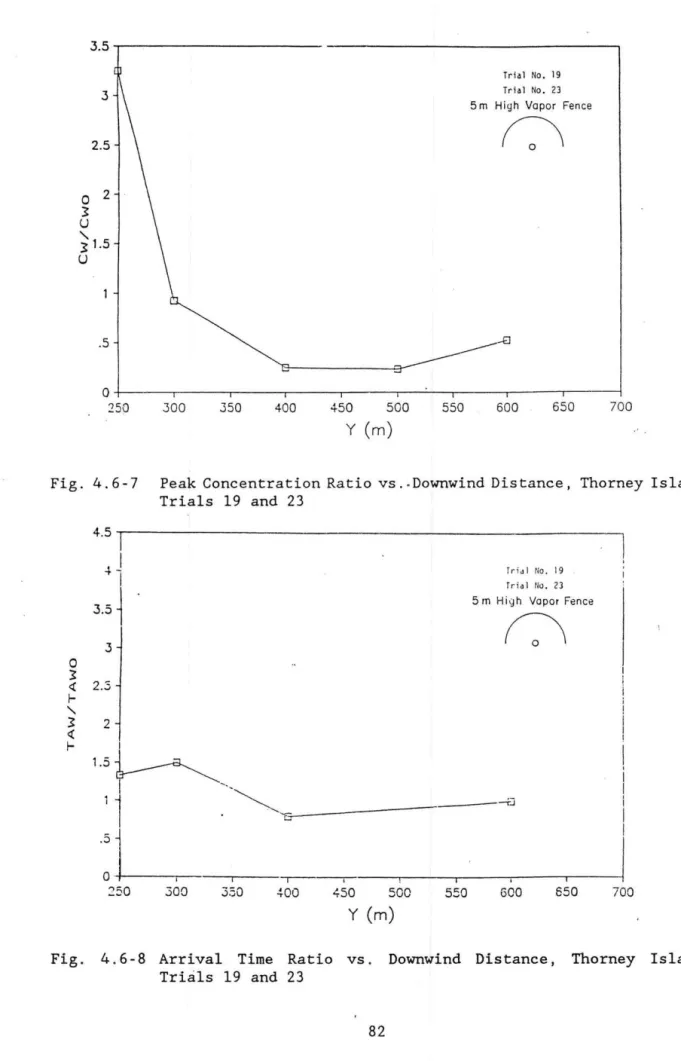
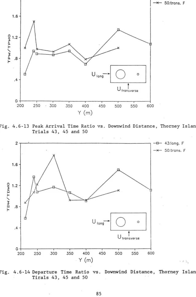
In the following figures Y represents downwind distance, the release location was always at Y - 200 m and the solid and porous fences were always located at Y - 250 m. During the continuous gas tests the wind approached either along or perpendicular to the longer fence dimension. Note that clouds are delayed by the barriers for time ratios greater than one and accelerated at ratios lower than one.

During the tests for instantaneous spills upwind of the 5 m solid fence it was found that the peak concentration ratios decreased from 0.4 to 0.1 downwind or the fence then slowly increased beyond 400 m (30 fence heights) (Figure 4.6-3) . Cloud arrival, peak arrival and cloud departure times changed from +20 to -40%, +SO to +200%, and +SO to +400 % immediately downwind of the fence (0 to 40 fence heights downwind). But farther downwind the cloud arrival, peak arrival and cloud departure times were -40 to -60%, 0 to -40%, and 0 to -10% of their no fence values (Figures 4.6-4 to 4.6-6). Apparently the lower wind . speeds directly in the wake of the fences initially slow cloud movement, but beyond the wake region the deeper cloud is advected with higher average wind speeds.

During the tests for instantaneous spills upwind of the 10 m porous fences it was found that the peak concentration ratios increased at the fence line (1.2 to 3.3), but then the ratio fell to levels near 0.2 at about lS fence heights downwind (Figure 4.6-7). Rottman et al. (198S) suggested that a gravity current might actually decrease its height passing through a porous barrier, which would explain the increased cloud concentrations detected locally. Farther downwind the turbulence generated by the fence increases entrainment levels and results in reduced concentration ratios. Cloud arrival, peak arrival and cloud departure times appear delayed in the wake region of the porous fences, but further downwind the ratios approach· a magnitude near one (Figures 4. 6-8 to 4.6-10).

The presence of a 9 m square building downwind of a spill site appears to perturb the instantaneous gas cloud much like the presence of a fence barrier. Enhanced mixing of the plume resulting in a more dilute and larger cloud produces reduced peak concentration ratios (0.1 to 0.4), and reduced arrival, peak arrival and cloud departure time ratios. If the building is not directly downwind dilution can occur but time ratios quickly return to one. An upwind building situated to one side of the spill will also result in plume dilution and negligible changes in time ratios.

A vapor barrier enclosure that surrounds a continuous source of dense gas appeared to increase peak concentration ratios directly downwind of the enclosure (2.2 to 8.0). Farther downwind peak concentration ratios decreased (0.3 to 2.0) (Figure 4.6-11). One explanation for the increased peak concentration ratios is associated with the tendency for the enclosure to restrain the initial upwind and lateral spreading of a dense cloud. A narrower cloud will produce higher centerline concentrations. The enclosures also seem to loft a small amount of gas to heights ~t which increased wind speeds advect the gas faster downwind; thus, one notes reduced arrival times in two of the three sets of comparisons (i.e. 0.1 to 0.2), but the third case produced peculiarly large arrival time ratios (1 to 9?). Nonetheless, peak arrival and departure time ratios ranged between 0.S to 1.5 for all three data sets (See typical Figures 4.6-12

to 4.6-14).

Conclusions:

The HGDT tests at Thorney Island provides tantalizing glimpses of the physics of plume dynamics downstream of a variety of obstacles. As expected normal meteorological variability produces perturbations in measurements which are often confusing as they are educational. Nonetheless, a few conclusions may be made from the comparison exercise.

@

Solid barrier fences reduce ground level concentrations measured downwind of instantaneous spills of dense gas. The additional mixing produced by the fence appears to have reduced effect beyond the wake region (30 fence heights).

@

Solid barrier fences initially delay the cloud movement through the wake region, but the cloud actually arrives earlier farther downstream.

@

Porous barriers may increase concentrations directly downstream of the fence; however, farther downstream peak concentrations are reduced.

@

Small buildings perturb a dense cloud much like a solid fence when placed directly downwind of the spill. Buildings placed off centerline from the cloud trajectory have minimal e~fects on time

ratios.

@ Enclosures placed around continuous sources of dense gas may increase concentrations downwind of the enclosure. Farther downstream the peak concentration ratios remained near one.

Table 4 . 6-1 Spill and Meteorological Conditions During Thorney Island Trials INSTANTANEOUS RELEASES

---~---TRlt'tL NO. : s.a. U10 VOL H (X:) f" UM Zo Fi- uN/UlO Zo/VOL-(1/~) H/UOL • ( l/!)) <><> f" /VOL -< 1/;,) V/L.!>

: _"/• "-:'.') " " H/•

...

.. 10-..

---·---

16. : lo f.0 '4.8 1500

-

- • 17 20 1. 4~ .0-4 17. 17 - - 1.50 20 : 1.'32 5.7 1'320 s 50 ... £. 20 1.65 .oa 16.0'3 ... o ... 02 1. '32 7 : l.78 '). 2 ;;:ooo

-

-

.07 2 -~~ .02 1.59 -

-

2.00 21 : 2.02 !).'3 2050 s so ... 1 20 .47 • 11 15.7 .. • ~9 !S. <) .. 2.05 a : 1. 70 2 ... 2000 -

-

0 2 • lb 0 1.59 -

-

2.00 22 : '4. ~(J 5.9 1400 s 50 • 12 2 .~9 .02 1. 79 .... s ... 7 1 ... 0 19 : 2.12 b ... 2100

-

- ... e 20 1.07 .oa 1S.f>2

-

-

2.10

2!) : 1.80 s.e N/A 10 50 "/A H/A N/H H/A M/ft H/A N/'A H/ft

1!> : 1.96 7.5 1'350

-

- .Sl 20 !>.5'3 .01 1£> .01

-

-

l.'35

2 .. : c: .0!) 7 N/A 10 so

...

lSO N/A H/A N/A H/R N/A H/A

CJ : 1. 7!1 l. 7 ;woo

-

-

.O!I 2 .0$ .02 l.59

-

- 2.00

2£. : 2.00 l.9 1970 CJ so .2 .. 2 .ot. • 1::!» 1. 6.0 .72 !I. 4)9 1."l7

1S : 1 .... 1 s .... 2100 - - .!>7 2 !).06 .07 1.56. -

-

2. 10

28 : 2~00 CJ 1050 9 so

.

;, 2 f..06. .O!> 1.E.:::» .7!1 ... 07 1.as

11 : 2.00 5.1 2100 -

-

"/A N/A 1.0L N/A H/A

-

-

2. 10

29 : 2.00 5.6 1950 '3 27 .25 2 1. 4!> • 041 1.60 .72 2. 1£. 1.95

---·---·---CONf!HUOUS R~LLASES

---TRIAL NO. : $.0. UlO VOL kflTE <C> H ~ L U"" Zo f"r u•/UlO Zo/VOL - ( l/~) Q/ <U lOML-2>

: ,../s; ... - !> .. -:=i/"11'.'

...

_{" "} ,../

..

...

..

M10-"4 Ml0-2

--- --- -- --- ---- --- --- ·-- ---·--- --- - - - ·--- --- -- - - - -- --- - -o-- --- - --- ---- --

~---~---.. t. ~.(\() ::'i."I Jt.>90 260 0 0 0 N/A N/A • 12 H/fi N/A 1.27

,~ _1.E.:') :.:-.s ₁₈₇₀ ::;,..o _{2.4' 2£>} s: .. _{• 15.} 10.00

0 10 .Ot. 8.12 2.27

.. 9 l.E.O .:

...

1907 26-0 2.4 S"'f 26 N/ f1 N/A .10 H/H H/A 1. 81

.. 5 2.00 2.!> 1972 26-0 0 0 0 N/ A N/A .OS H/A H/A 1.88

.. :=i 1-~~ 1.5 1899 2f>5 2 .... 2£> 5'4 H/A N/A .07 N/A N/A 2.c;, ...

so 1. :=ia 1.6 1&00 270 2 .... 5.q 26 N/f1 N/A .07 H/A H/A 2.e 1 !>8 : 1.£.0 :=>.8 10t.7 280 0 O O N /fl H/A .25 N/A H/A 1.2!>

'7 : 1.60 ,_,.. 10s1 255 2.... 2t:. s... .::i':I 10.00 .20 .11 e.o9 1.25

---.---~---~---~--r .. iAL NO. : Fr- VOL/(H•i.l..cL) H/VOL-(1/!)) U/'VOL-(l.I!)) L/VOL-(1/::J)

---

4b _'3.2£. - 0 0 0

''

...

_

..

,

_.55 • 1 <j 2.11 ... ,:,a .. 9 s ... , _{.57 .19 ""•!IS} 2. 10 "iS _2.07 - 0

"

0

..

,

2.!)6. .56 • 1 '3 2e 10 .... :!)£> so 2 ... • 5~ .20

...

2. 1 ..

,8

20.00

-

0 0 0 37 15.7:> .So • 1 '3 2. to .... ;,7 ---~---~---~----74

Table 4.6-1 Obstacle Configurations During Thorney Island Trials

INSTANTAMEOUS RELEASES

---~~~---~-TRIAL NO. MINO

DIR. <DEG> Fr CONFIGUiitAfION

---~---~---~~---16 . -14.;:, -~5 UNOBSTRUCTED 20 -E>.5 -~ 5,.. L.IALL AT 50H

.,

... s.3 • 1 ... UHOBSn~UCTED 21 -6. 1 • 15 5,.. L.IALL AT 50'1 8 -15.8 ' .09 UNOBSfl<'UCTEO 22 -7.E. .11 5,.. L.IALL AT so .. 19 ~0.2 -~7 UNOBSTRUCTED

2~ 29.6

....

;:, 2•10"' POROUS FENCE AT SOM

1~ !S0.8 .51' UNOBSTRUCTED

2 .. 28.8 ."46 ""~10" POROUS FENCE AT SO..

CJ -26.9 .OS UNOBSTRUCTED

21& 5 .0"4 9,.. SQUARE BLOO• 50"' 00&..IH RANGE

15 .8 .72 UNOBSTl".UCTEO

28 ... 1. 9 .82 9,.. SQUARE BLDOs 50"' AT ""5 OOMH RAHO£

11 6'3.6 .29 Ul'IOBSTRUCi"ED

29 27 - !J2 '9,. SQUARE BLDO, 27,.. AT - :::10 UP RANGE

---CONTINUOUS RELEASES

---~---~---TIUAL NO. ~IND

DI~. <DEG> Fr CONFIGURATION ---~---~---.. ft 76. f> • 12 UNQEfSTRUC r ED :n 1.8 _{- 1'.l} 2 .... FENCE LONGITUDINAL ""9 1.2 .11 2 • .q'1 FENCE TRANSVERSE <lfS -~4-5 .OS UNOBSTRUCTED

..

~ 10 .oa 2 ... ,. FENCE LONOITUDINAt..

so "42. '9 .OS 2.~ ... FENCE TRANSVERSE

38 -25.1 .25 UNOBSTRUCTED

:::17 -26.5 • 17 2.~ ... F"ENCE LONGITUDINAL

---

·r~-.

\

,.

\

\

\

·1F4--1

!F4

_I

y 3 : F5

TT

I

I

I

I

I

I •

F~

I

y 2 3 5 10 9

\

:-.::::

...

_... , D

...

' '

_'

'

_'

\

'

'

'

.

\ J ' - I ,-, ', GRID NORTH t

I

/

I \ ' \ ~· I I ' ' et-' _' •I _{r1 I I} / ' ' _\' eF4 , c I \ a:

I

I I , \ I

I

\ \ I I I

71-\ \ eF2 eF2 1F2 a'F2 / •Fl

\ \ 7 I \ \ •F2

t ,' /

\ \ I F2 I \ .. F2 • F2 • F2 F2 / •

I

' \ I I \ \ I

I

\ \

· 46 F2 \ e F4 e F4

J' / /

F41 I e F4 \ \ I I \ \ I I \ \ I I \ \ I I \ \ F4 F4 I \ ~F4

r-

7

_,F4 \ \ /, I I

\ \ t

_{\ \} F4 I I I I

1

F4 ' \ I 1 \~Fi:\ iF5

I /

FS

\ \ I

I

I

\

\ \ Lf-11 I

\ I

ti.

_J

\ \ I I \ \ -\ \ I I \ \ I I \ V I e V \ I \ I \ I • , <

I

I \\

t

1' "I I A •\I

I

) ,. m ' I \ SCALE • "

I

I

t \

ol

I I / \ \ I I I •F2 E _{•F2 •F2} 5 _{•F4 •F2} 4 _eF4 3 2 0 1 2 3 4 ~ 6 7 x

Fig. 4.6-1 Spill Configuration and Measurement Grid, Thorney Island Trials 76

Y(m) 300 . 250 _(a) 200 ~RELEASE POINT ..._ ____ __._~---"---~ X(m) 300 Trials 1- 19 Y(m) 300 2~ 400 500 5m vapor fence 50 m Radius (b)

I)'',· 250 y (m) 2.4 m vapor fence RELEASE ?OINT

f

(see Detail A) 54m

I

19m X(m) 200 300 500 19m Gos Container

I

i

L

f

--1 25m

150 _{Fence longitudinal (Trial 38 without fence)} Y(m) 250

-119ml

I 200 ₃₀₀

I

rt\

I

X ( rn)

I

500 150 Fence transverse Y(m) 250 200 300 150 _{TriaJ 45, 46, 47} X (m) 500 (a) (b) (c)

Fig. 4.6-2 Obstacle Arrangements, Phases II and III, Thorney Island Trials

:.: Y (m) _{. ...} · 300 250

RELEASE

20.0 300 Trial

Y(m)

300 250 200 28

r--45°

, y

0

9m square building POINi- 1

/,>

~

50m

,VI

X(m) 4\..--0 500

<

1 RELEASE POINT

27m

W

01,

₀

_I

9m square buildinQ

Y::o

0

L..-~---"----~_.~---"---~

X(m) 300 400 500 Trial 29 (d) (e)

Fig. 4.6-2 Obstacle Arrangements, Phases II and III, 7horney Island Trials

1.4 1.2 0 3 u .8

'

3 u _.6 .4 .2

ol

250 300 350 400 450 .500 y (m) Trial No. 8 Trial No. 22 5 m High Vapor Fence

G

550 600 650 700

Fig. 4.6-3 Peak Concentration Ratio vs Downwind Distance, Thorney Island Trials 8 and 22 1.6 1.4 1.2 0 3 ~

f-'

₃ .8 ~ f-.6 .4 .2 0

:so

JOO 350 400 450 500 y

(m)

T rt ct l llo. 8 ; rid l No . 22 5m High Vapor Fence

G

550 600 650 700

Fig. 4. 6-4 Arrival Time Ratio vs Downwind Distance, Thorney Island Trials

8 and 22

4.5

4 Trial No. 8

Trial tlo. 22

3.5 5 m High Vapor Fence

G

3 0 3 2.5 0..

I-'

₃ 2 I a. r- _il.5 ! .5 Q+-~~--,--~~-'-,-~~~~~~.--~~.,.--~~~~~-,-~~-.-~~--j 250 300 350 ~00 450 500 550 600 650 700 y

(m)

Fig. 4.6-5 Peak Arrival Time Ratio vs. Downwind Distance,.Thorney Island Trials 8 and 22

4.5 "'

A

..,. Tri d l tlo . 8

Trial ~!o. 22

~ 3.5 5 m High Vapor Fence

3

G

0 3 Cl 2.5

I-'

3 _Cl 2 I-1.5 .5 O-r-~~-.~~-r~~--,,..-~~-,--~~-..-~~-,-~~-,.-~~--r~~---; 250 JOO 350 400 450 500 550 600 650 700 y (m)

Fig. 4.6-6 Departure Time Ratio vs. Downwind Distance, Thorney Island Trials 8 and 22

3 2.5 0 2 l u

'

3 1.5 u .5 Trial No. 19 Trial No. 23 5 m High Vapor Fence

G

Q+-~~~~~~~~~~~~~~~~~~~~~~~~---.~---;

250 JOO 350 400 450 500 550 600 650 700

y

(m)

Fig. 4. 6- 7 Peak Concentration Ratio vs .. Downwind Distance, Thorney Island Trials 19 and 23 0 3 -t

j

I

3.5.

~

3 ~ 2 . .5

1-,

3 ~ I-2

1.5~

Tr i JI No. 19 Tr i a 1 No. 2 3 5 m High Vapor Fence

I

' ,

11

.

~a~---+J

.5L

_{0 . I}

---.----r-250 300 3.SO 400 ~so 500 5.50 GOO 650

y

(m)

700

Fig. 4. 6-8 Arrival Time Ratio vs. Downwind Distance, Thorney Island Trials 19 and 23

4.5 4 3.5 3 0 .? '1. 2.5

I-'

l _{'1. .} 2 f-. 1.5 1

·:L

250 300 350 400 450 500 550 y

(m)

Trial No. 19 Triul llo. 23 5 m High Vapor Fence

f:'\

600 650

J

700

Fig. 4.6-9 Peak Arrival Time Ratio vs. Downwind Distance, Thorney Island Trials 19 and 23 4 3.5 3 0 l _2.5 Cl

I-'

l 2 Cl I-1.5

I

.51

0 -+-~~-,.-~~-.-~~-,--250 300 350 400 450 500 550 y (m) Tr i JI :10 . 19 Tr id I :10. 23 5 m High Vapor Fence

G

600 650 700

Fig. 4.6-10 Departure Time Ratio vs. Downwind Distance, Thorney Island Tirals 19 and 23

8 0 6 3

u

'

.J 3 4 u 2

I

)/

1~

0 -+-c---,----,---.--· 200 250 300 350

Ulong{Q3

t

LJ

transverse

~~l

· : _ K

-r-J

400 450 500 550 600 y

(m)

Fig. 4. 6-11 Peak Concentration Ratio vs. Downwind Distance, Thorney Island Trials 43, 45 and 50 200 250 300 350 400 450 y

(m)

500 550 600 43:1ong. F 50:trans. F

Fig. 4. 6-12 Arrival Time Ratio vs. Downwind Distance, Thorney Island Trials 43, 45 and 50

2

--r---.

-a- 43:1ong. F ~ 50:trans. F 1.6 0 _{3 1.2}

I

a.

f-'

I

3 a. .8

f-U

long-~1

0

0 .4

t

LJ tron 5verse 0-t---.---.---..----~----r----.---.----l 200 250 . 300 350 400 450 500 550 600 y (m)

Fig. 4.6-13 Peak Arrival Time Ratio vs. Downwind Distance, Thorney Island Trials 43, 45 and 50 0 3 0

f-'

3 0 f-2 . - - - " - - - , -e- 43:!ong. F -*- 50:trans. F 1.6 1.2 .81

I

_U

_long-I

₀

0 .4

i

_t

ol

LJ transverse 200 250 300 350 400 450 500 550 600 y

(m)

. : ...

Fig. 4.6-14 Departure Time Ratio vs. Downwind Distance, Thorney Island Tirals 43, 45 and 50

4. 7 "Wind Tunnel Modeling of the Thorney Island Heavy Gas Dispersion Trials," Davies and Inman, 1986

Experiment Configuration:

The purpose of the Davies and Inman (1986) wind-tunnel tests was to obtain a large data base of laboratory simulations over a range of model scales typical of those used in hazard studies on prototype installations. Scales ranging from 1:40 to 1:250 were used to simulate 34 trials from the Thorney Island HGDT project. A total of 86 laboratory cases were produced. Typically, 10 repetitions of each wind tunnel run were required to map the concentration field for each simulation and to provide point to point comparisons with the 10 to 20 "ground level" (0.4 m high) sensors used during the field trials.

The instantaneous spill cases of the HGDT project were simulated at scales of 1:40, 1:100, and 1:150 using a collapsing wall type container to simulate the prototype collapsing bag. A large grid of sensor locations were used in the laboratory to enable concentration contours to be prepared from the laboratory""measurements. Concentration measurements were made in the laboratory with low-volume hot-wire aspirated katherometers. These instruments permitted measurement of concentration

time series at each sensor location.

Davies and Inman provided some comparisons between their laboratory measurements and the Thorney Island field results. This report examines the data further by the Surface Pattern Co~parison technique described by Meroney (198.6b, 1987). The emphasis here is to analyze the results to establish the level of confidence which can be placed in laboratory simulations.

During the field study there were a large number of uncontrolled or poorly specified variables, which have effects on the resultant concentration field, that are not completely accounted for by either a physical or numerical model. The full-scale wind field is typically nonstationary, the source conditions are only approximately known, and the modeling method itself introduces errors. The Surface Pattern Comparison method estimates how much the predicted concentration contour pattern must be shifted in space to cover all of the observed values. This is done by comparing observed and calculated patterns over increments of decreasing spatial resolution. The result of such a comparison is knowledge of what percentage of observed concentrations are contained within increased areas of spatial resolution as specified by their angular displacement observed from the release location, delta theta.

Results of Comparison:

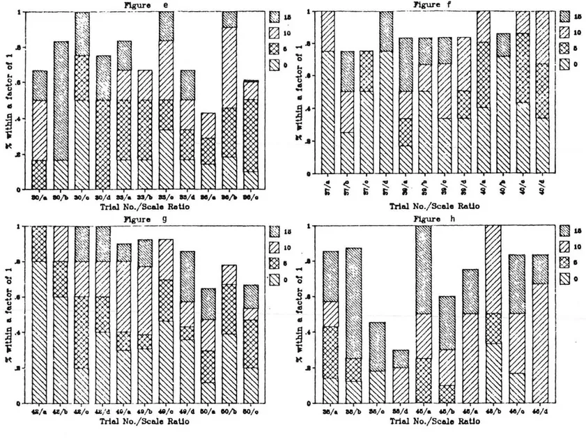
Table 4.7-1 lists the prototype and model conditions considered by Davies and Inman. The peak concentration contours at ground level measured at full scale and during the laboratory simulation are plotted together in the Davies and Inman report. These data were used to produce Figures 4.7-1 to 4.7-3 and Table 4.7-2. Figure 4.7-1 shows a typical plot

of f-N, the percentage of field data predicted within a factor of N by the laboratory data, versus angular displacement, a measure of spatial resolution. All trials were regrouped for comparison as follows:

1. Unobstructed instantaneous releases (Figure 4.7-2c),

2. Instantaneous releases with wall or building (Figure 4.7-2d), 3. Continuous releases with fence enclosures (Figures 4. 7-3a to

4.7-3c),

4. Unobstructed continuous releases (Figure 4.7-3d).

Scale ratios of 40, 100, 150, and 250 are denoted by ##/a, ##/b, ##/c, and ##/d, respectively on these figures.

Most laboratory scientists expect that as model scale ratio, LSR, . increases the quality of the physical simulation may decrease. This

decrease results from mismatch in turbulence size and strength, exaggerated dispersion due to microscopic transport, and mismatch between buoyancy and inertial forces in the model. Thus, one expects some evidence that the quality of simulation decreases as one changes model scale from 1:40 to 1:250 (from cases a to d). It would be valuable if one could quantify the loss of accuracy as a function of model scale.

Unfortunately, close inspection of the data reveals no consistent pattern of error variability with model scale. Tests 42a, b, c, and d; tests 8b and c, tests 38a, b, c, and d show the expected decline in model reliability. Yet tests 49a, b, and c; tests 30a, b, and c; tests 33 a, b, and c show the opposite trend! Other tests display an irreg~lar rise

and fall of accuracy with scale ratio. · At this time it is not known whether this is evidence of normal statistical variability, experimental errors, or fallacies in the similarity theories.

On a positive note, most of the data compared within a factor of one for angular displacements of 15 to 20 degrees. Similar comparisons between field data and many numerical models require angular displacements exceeding 45 degrees. Also results from continuous spill experiments appear to compare somewhat better than the instantaneous spill experiments.

Conclusions:

Laboratory simulation of dense gas behavior near obstructions appear to be reliable in the sense that predicted concentration contours do not require major modifications to reproduce field data. Based on this Surface Pattern Comparison analysis no limitations could be placed on the largest model scales which might be used to simulate dense cloud behavior.

,.-I I"--->I I ._, I ... 1 I ::001.11w~~~~~~~~~~ocoo~: ~: QQOQOUUOOO : i-1 I •Ill I 1 1n~,....,~,...n111111nN..OL111\.~..o .. ..on1 I I 11\.nnal~O~NnOl\.lllNl\.~~ ... T•I 11' I''•••, .,•• t ' •'• .•••'•I Is 11\...0~..0..0l\.n .. ._al'l'NOll\olln'-T"" I •• I N""N""-~"~~N~-

I

IQI t t ~ t I I I I I I I 1•N•O~T..o..o:!D ... no1 I 1:'1'111n:-~T='-!DnNl\.O .. .,~,,, ' I I • • • • • • • • I • f • • • I I I • I .

I " I

•'I'

T N 0 'I' r1t.'111..0 'I' N 'll .f' !D .. "'" '- n I 1 • 11\.•0~r-.. ~~..00111~~,,., .. ._.,, IQI 1..o~'ll~=~~~~~-,...To~n:o•1 1v 1~ - ~n~~~n~N~N~~n~n1 : : .. I I t I I II\ I 0 0000 0000 I 1 .. 1oocooooooocooocoooo1 _{1:11 1':>000•0 •0••••000••••01} 1 "\. I • • • • ~ • • ·fJ ~ 11'1 \II • • • D tf'I T "'11 • I I• 1~..0TOC~~~"~T~~O-~~"'l'I ·~ l~TDC~hT~r..oTcno~nN~!DI I~ t~---~~nn-~-~T~~~N~-· I I I I I I I I t I 10000000 01 m 1111~"'""'"111~11100000000000'1'1 """ I • • • · • • • i t.r. l/l "' U"l 0 0 '.J) w'\ w' ..,. " • I ~ :~~~~~~~~~~~~~~~~·~~: I I •I I

,,

NI 011 El~!D~!D='ll'll!D=:!D~'ll:!D!D!D'l)!D UIOOOOOOOOOOOOCOOOOOO I •• I • • • • • • • • ' I • • • • • • I I CI 1.11 .. 1 lo- [ I I 1%:' I I I I I I I I I I I I I I I I t I I l 1 xn t I I I I CI t I I I I . : ggggggggggggggggggg l ..Jf'tl I I t I I I I I t t I t I I I I I I I c11ooo~oooocoocooccooo ~EICO~>COOOC~~ ~~C:~:~ "'I 1cor~~~~--~~oo~~~rr•1 INN .. _ .. _•NN•-NN•-- .. •Nr I I I I I I I I I _{• l'l'O..O ..} : I Tnn~T~~~~~on111~NI O•!NNNN!D~T~~~vnnT~~~TNI ... , f S a e . ' e ' e SI. I I I e e f •I. :::1 & I I I I I I I I :~ :~i~~~~~~~~~~~888~~~: f 0 . . . I • • • • • t • • • •I l•,INNNN~~~~~~~nn~~~~~-· I ::I It I .. I I I I I U I: I I • M~ I I 1!..).I I 1,..._, I I U"" I I I U~ I I 1~:100000000000000000001 !V1c.:1,...~nnNNN--~roo~oooo~1 I vo I • • • • • • • I ' I • • I • • • • • • I I 1• .. NNTTTNN .. •NNTNNNN•I I I I I I I I I.I• I I 1 ... 9\ I I I lo.> I I 1 .. '-I I I u~ I I II.I.) I I 1~::oooooaoo-:ioooooooooo1 l~~l~~nnNNN·-~~OONOOOOQI Iv.;, 1 • • • • • • • • • • • • •. , • • • •I I 1-•NNTTTNN••NNTNNNN•I I I I I I I I • I I 1~0100~0 '~ooooooeooeo 1 1..1-100000000000000000001 I·~ I I • • •O ' ' I f • ' . ' • I • • 11:>' 1_{1\ t '~ -:, I 0 .:. ~ :> •} ~ r:> ~ ~ 0 0 0 0 0 0 C 0 ':> • w•~c.:1o~c~oo~o~o~=~~o~o~o ~· ---~·-""~---~---~ .::1 ~~ i.t I 0 QI I Z I ' 1111 z: ::JI 0 0 I .. ~: ~ ~I ;.: .. 1..10 Z I 1%:':> lL I '"4-1- 1 C.: '-. . \/\I._~ Z: I 0 .. 1 u 1..J~ _I.JI-I I ,...

.

IO..JI LllWWLll~OO . i..i.. I :~;:1.11wwwa~o~~~~ww1.11wi..i..i..i..ooooooooooooi..i..i..~~ooooi..~i..~i..i..4i..:

I: i: I I

1 &.i- I I

: ~:~~-~'l'~TN"'"~~~O·N~·~•n~~ .. ~~~--~TNTNO• .. On~N'l'nn•~-~,, I~ :~~~~~~~~~~~~~~~~~~~~~~~~~~~~~~~~~~~~~~~~~~~~~~~~

1• 1-n•!DNT-~111~=~o~~~N~~~~~ .. ~~=..o~o=..on~h .... ~o~~ .. 0NO!DT=h

I• IN~~ N~~ " """' "~ N~~~" ~~ ~ ~ •~ ~~~ ~

I IC I

: ~ I

: : •• ., .. ~O~Nng:111~Nn~~~~lll~O~hTn~n=--~~-·~n~~~-~N'llTOOO

1 1~~111~o•T~n~T=~~=,...~n .. n-~'"~no~o~~~~O .. ,•nTon·o~-~-~~=

• I I • • • • • • • • I • • • • • • • • • • • • • • • • • • • • • • • • • • • • • • • • • • • • • • • •~ •~•con~o==~~~•·•7n~~~n~·~N·~-~ .. ~·-Nn~ooTn~N~'-"-~" I. 1Tnn~=T~~~~noo•111NnN~~Nl\.!D'-NN~-~~•n~T~'n .. -~TT~~ .... Tn IQI l~N· nn .. ~N-=N• ~N- Nn• !DN• ' " ON•~-=N~ ~ .. N. •N• '"

.

... ... . ... ... I I I I I I I C I I~ I :~ :goo o o o oo 80000 o o o o o t ' I ,_ O O O O 0 0 0 0 0 0 0 0 0 0 :l 0 : 0 '' 0:; 0 :l 0 0 0 0 0 0 0 0 0 0 0 0 0 0 0 0 0 0 0 0 0 0 0 0 I • I 0 .-. .,.,.. O ...,. ·~ V 0 i:1 0 0 -1' 0 ::: ;~ !' r 4 •: ~ ~ ~ ·.D ,._ T ::: 0 0 '4°'. fJ 0 ':l ... 0 :) -.:> 0 f1't C ':' 0 0 i"" 0 -:> 'j ~ 0 0 IL l .. N•l\.n=TN-'l'NN~TNT-~nN..on·n~111Nn~~N-nNl\.N•~n-NN..On• .. ,,N '" ' I I I

,.

I~

,

..

0000000 00000~00000000000 ooooNNNN4~400000000000000000000111~111~~oooo~nnnn•" .. NNNN••••• •·~~'"~111~~~--·•NNN~~~~lll • • ·~••••••••••••• • . . . I • \I • • • • • ' • • • • ' •N<"lll~N- ~ ... ",._ ... NNN 1111

,

... I I ..

!

Q ~ : I t =~~~~=~~~!D~=~~=~~~=~=~~==~~~~==~~=~~~=~~'ll~~~~~~~I 1 _I u _{I • • • • • • • • • • • • • • • • • • • •} oooooooooooooc~cooooooo----aooooooooocoooooooooo1 I • • • • • • • • • I • I • • • l • • • • • • • • I • • ~ : : I I C I I I •10000000000000000000000000000000000000000000000001 1 11ocoooooooooooooooo~ooooooaooooocoo:iooooocooooooo1 I ' I I • • • • t • • ' • • • • I • • • • ' • • • • • • • • • • • • • • • • • • • • • • • • • I . • . • • I 1~n100000000000~111111~000000000000~~~~~~111000000000000001 1~11~..0•..0TTT'l'••-~~~~~=~=~~ ~ ~----~~~!D&DD•4~·~~~..0D..0~~ .... I l«XINNNNnnnnnnnNNNNNNNNnnnnnnnn• .. --NNNNNNNNNNNNNNNNNI Ill: I I I I I : . :gggggggggggggggggggggggggggggggggggggggggggggggg: 1..Jt'\I t • t 1 t 1 o • • • t t I I t 1 t I • • t I I I t • • • • I I • 1 t e t I I I t t 1 o • t I I ti 1011nftrnacaonnn•·--~~ .. ~~~~~cooonnn~r~~~~ooco~ .. ~~~~001

I ~ f. I C '.:l : ~ ..._ ,.... lti.. '-U -~ ..: It" :" :" ':"! ..J ·.IJ' .J l.D .:l ':.I :) :J ~ ~ ..: j ,._. "'- ,.,_, ,.._ :"-1' (!'I !'\.. -~ ~ :"' 1" 1" " '= 'J ':: = ':) C 0 I

I l~~~~~»~O~~r~~~~~~ ~ ~~~;~n~~~rr~~DD;~~TTTl~~~~~~DOI ~ I ..,_..,.~,...,.. .. .., __ ... _.., ___ ,.. _ _,,... ""'..,"""'..,_.,..,.,..~..,.,. ... ,....,..,..,.~.,. ... .,. .. , ,t.,..- ... I I I I I I I I I I I I I I I I I I I . I

I. !on~ .. OT•~~-~ .. N~OOO .. TN~ .. ~~ .. ~OV~~Nn .. N..OnNn~-•nON~'l'mNI

10•1~TnNl\.TnNTnN~nNN~nnN~~TnTnNNL11nNNTNNnNL11nNNN~TnNTNNI I .. , • • • • • • • • • • • I • • • • • • • • • • • • • • • • • • • • • • • • • • • • • • • • • • • • • I I :::1 CI I I I I I I I I I I I I I , .. 1ooooooooooooooooooooooooooooooooooooooooooooovTvt 1 • 1nnnn~o=~'l'T'l'NNNN0~==~=0~•·•-TT'l'Vlll~~nnnnnn~~~lll~h~~• I 0. t • • • • • I • • • t • • I • • • • • • • t • • • • • • • • • • • • • • • • • • • I • • • • I • • I 1•,tTTTTNNNNNNNnnnnnnnn~~~~nnnnnnnn• .. •NNnnnn .. NNNN-••1 1:::111:1 I I I I I I.I 1 I I I W" I I I:..> I I '"",...' ' I U,. I I I W:'.> I . I ·~~1oooooooocococooooooooooooooooooooooooooooooooooo1 l\/\~ITT'l'T~~·~ooo•..o~..o~•~4TTTTNNNN•~..o~oooooooooc~~~·OOOI I vo I I • • • I • I . I • • • • • • • • • • ' • • • • • • • • • • I I • • • • • • • I • • • • • I • ' ' I 1• ... ~-NNNNNNN ... ~ ... ..,..,.., ___ ..,..,..,..,..,..,~ ... -~NNNNNNNNNNNNNNNNNI I I I I I I I U'-1 I t ... 1\1 I I II.> I I l •t-1 I I u .. 1 I l<U::J I I 1~;1ooooooooooooooooooooooooooooooooocooaoccoocooooo1 ·~at'l'TTT4..0~~··~~~·~•D•~TTTTNNNN..O~~~nnnooooooa••••TTTI I \IQ ; I • I I o I f t t I I I I I I t • 1 I t I I I I t I I ' I o I I I 1 I t t t I I I t I I t I I t f I 1-•-•-•• .. -• .... ••• .. -~ ... NNNNNNN•• .. •-• .. I I I I I I I

11.1101 ooo eoo oo ooo ooo ooo ooo coo oo _{1J-1oocooooooooocooooocoeoooooooocoooocooo~ooooooooo} o ooo ooo oo

' :: ~ I 0 I • ' 0 • f I 0 • I 0 ' •.• 0 I I • .:) • I I 0 • • I 0 • • • ~ • • 0 • c ' . ' 0 0 • • ' 0 • •

IU<tl •COO •O~O •00 •000 •000 •000 •COO •000 •00 •O •·000 • •000 •00

1~ac1oo~~oc~~~o ~ oo~~oo~~oo111~00111~00~~00~00eo~•ooo~~oo~ I IV••N'l'••NT .... T•-N'l'-•NT•-N'l'--NT .. -NT••V•T•-NVT•-NT .. • ~I I ~:

.

: 1: I 0 I WI %.t _. t ' I WI Z I QI I 0 I I '"' VII i-t ::)I 0::1 0 I QC I

~·~~1oooornnr~~~~~ .... e ~~~•~roooO~NN ""~~~~..,~~r~ rooo

z:1~c1nnnnnnnnnnn~nnnn nn"nnnTTTTTTT TTTTTTTTTTT T~~~

_, __ ,,,,,,,,,,,,,,,,, ,,,,,,,,,,,,, ,,,,,,,,,,, ,,,,

._l~~l..J..J..J..J..J~~~~j~jJ..J..JU UU..Jj..J~~j~~~JJ J~UUUU~UU~• lo-~~~ %11--Zl~~ll.i..~~i..~~11.~ll.~~i..:::l :::l:::l~i..~~~i..~~~~~ ~~:::i:::l::J::J::J~::J~i.. i..~i..i..

CI 0 I

U I \,I I

Table 4.7-2 Summary of Surface Pattern Comparison Results

for Thorney Island Trials

-~---_Seal• <O•~•tt\I (O•n•lt\I ~otnt• Int•rc•pt: o' fh•ta• D•9~••• Con#iQur"••lort O•t:• : r.-t .1

: Con,louratton/Hft. ••tto ••tlo>~ •atto>n Co"par•d f-1 · '-2 ,_5

---~-

---rtior"•\I I 11 I and 'l•ld ( )

i

11od•l o•es>

-

Ul/08 too t.?' I.?

•

10 7.'S Ul/08 I lSO l.1' 1.r r 21'.S r . s Ul/12 I 100 :r., 2.,

•

2S 15 Ul/12 I ISO 2., 2., 8 15 u.s Ul/lT I o40 .... 2 .... 2 r so :io Ul/11' r 100 ... . 2 4.2 8 ,2.s 15 Ul/lT _' 1o; o .... 2 ... z 8 2 '. 5 7.5 Ul/l• I 100 2. l 2.1 10 2 0 7.S Ul/l• I 150 2. l 2.1 10 20 10 5M-S0/20 I 100 1.• l.•

..

15 5 511-50/ 2 0 : lSO l.'1 l.9 5 10 5 SM-S0/21 I 100 2 2 5 2 0 ~11 - 50/21 I l ~ O 2 2 12 :.: 2.s 12.5 511-50/22 I ISO ... 2 4.2

..

25 17.5 •B-S0/20 I 100 2 2 1' l 'i T.5 _,B - 50/,;:e I ISO 2 z

..

lS 10 I •e-2T/;::., I trio 2 :z 'I ·20 12.S '90-21/ 2') _' 150 2 2

•

2T.'S 12.S : · FL/'O I 40 1.4' l ...

..

22.5 u.s FLl''O I 1'10

....

1 ...

..

.. 0 FL/'O I I S O

...

l . ..

..

12.S s f"L/'O : ;?SO 1 ... l ... . 4 1T . S FL/-'' I o40 l. .. :z.s

..

2S FL/'' : JOO

....

2.5

..

11'.5 12.s FL/'' I 150 1 . r. z.s

..

lS 10 FL/.,, l .zso l." 2.S

..

2S 12.S UJ/'4 I 40

...

t.•

•

2.l.S FL/'6. o40

'·"

2 ~ :1 0 r.s ,.L/.,o; t o o t.• 2 11 I'S 1'.S FL/::i6. I ISO l . ' 2 10 :10 FL/'T I •o l. ..

....

4 7.5 .,,s FL/-'1' I H•O l. f> l.t.

..

72 . 5 0 ,.L/'T 1'50 i.r. l ...

..

lT.5 2.S F'L/31' I 250 t . ' l .t.

..

15 0 IJ("/~11 l o40 LL l .t. 1' 20 r.s UC/,11 100 l.'-

....

•

2 5 10 UC/.,11 150 1 . 6. l ... l l ~o 2 2.s ucr:ie 2'50 l.f. 1.t. 10 2r.s 15 ,.L/''9 •o l. ..

...

..

22.S 7.5 ,.L/''I tot> l . '4

.

...

..

20 10 FL/3., ISO 1.4 1. '4

..

22.s ti) FL/''9 :t'SO 1. 4 l ...

"

17.S s FL/"'0 .. 0 t. z 1.2 5 1' . 5 7' . 5 ,.L/•O 1'10 1.2 1.2 r 15 0 FL/<40 150 t. z 1.2 1' 1'.5 2 . '5 FL/40 250 l. 2 1.2

..

10 10 FL/42 •o t ... 1 ... 'S 5 0 ,.L/42 100 '·'

....

5 r.s 0 FL/42 \SO t . t. l ... ~ IS ts FL/42 250 I.'- l .t. 5 12.s 7.S FL/<4, 40 1., 2

"

5 5 FL/<43 10 0 l., 2 12 ;;- o r.s FL/4' lSO

l.'

2 12 2 0 · 10 UC/<4S t .. 0 2 2 7 u 12.s UC/ 4 5 t 100 2 2

,

... Z2.5 I S 10 UC/'46. I 40 2 2 5 :n.5 s llC/46 I 100 2 2

..

10 10 UC/-16. I 150 2 2

"

17'.5 10 UC/.,fo I 2';0 2 2

..

27 . 5 10 UC/47' .. 0 2 2 15 15 2 . 5 ,.r, .. ., I .. 0

....

2.s 14 20 2.s 2.s F'T/ -l 'J : 100 I." 2.s 1-4 ;::T.'S 10 Ff/°"'J I 150

..

,

z.s 1o4 2S 10 Ffl'<49 I ~ !' O I.E. 2.S 15 21".~ HJ ,.T/'50 I .. o

...

2 :n.s .,r) JS Ff/0-0 I 100 l.<4 2 1r ~2.S 20 150

...

2

,.

:')5 10 ,.T/SO I ---ut • u~ob•truct•d ln•tant•~•ou• r•l•~··

S M-SO - s" Mall at so"

98-50 • "" squar• bldQ• ~O" at •S d•or••

~~ - ~7F:n:: ~~~~:u~!~~t 2T" at 30 d•9r•• UC • Unob•truct•d contln\lou• r•l•••• FT • F•nc• trav•r•• 89 dOUft f"ar>O• up r•no•

Ground level

-ii-f-1 1

I

7

II .. • .. II I ..

7

l-it-

f-1

--- f-1 --- f-2

insta11taneous release

.1-I I in unot:.s truct~d flat tcrra in I .a

( tr id 1 no. 8)

with LSR .;; 100

.1 A Ground level

:z:: :z: instctntaneous release

J..

J.

in ur1obs true ted flat terrain

(trfal no. 8) -' A with LSR = 150 ~ ~ Q 0 G S 10 1~ 2Q 2:1 JO Q ~ 1G 1~ 20 ~ lO . DEGREES DEGR£E -e-H

'I

77 . . .

1--f-I

--- t-1 --- f-2 _,,._ f-~ -.... t-:. ~ ~

A Ground level .I Grourid level

z ~ristcrntaneous releQse :z: instc111tdf1tous release

.!,. 111 unobstructed flat terrain I fn unobstructed flat terrain

(tridl r10. 12) - (tried no. 12)

"' with LSR

=

lQQ A with LSR "' 150

~ ~

Q Q

Q i 10 " ;o l:s ~ g ~ 10 " 2Q ~ .X)

ot:GREE ()(GREE

Fig. 4.7-1 Surface Pattern Comparison Results, f-N vs. Angular Displacement

....

-

0 ~ " ... ₀ .I .a O' .. ,,,., P)1 '>i'I Pj>'I

..

0

'8/• ~,~ .W/o .a/d ~/• ~ID "'/• .. ID .. ;o 4'0/4 TrioJ. No./Scalo Ro.Uo

~uro . c

IS/ll O/o 1&/1> 12/o 17/D 17/o 18/D .8/rJ H/•

TrloJ No./Scala R4tio

~.,

...

~·

~

...

[S10 ...

-

g Jo.

.s ..

₀ II

...

_..

~··

i ~

..

---

~e __ b __________ _ D I I) 'i' H • ) ' • ' M I I - ... .. . . I I I

~

'°- '

~ 10

~·

....

..

~ 0 'O

_...

.s ..

0 II

...

II

~-·

i ~

..

~I• ~ID ~/o '-i/4 60/a 60/D IO/o 1'rlal No./SCAlo Ratio

~o _d

DI l){H l ' j ,. l ' j ., l ' i ' " ' ' •

I .. ,

H '"tit' t I t f ··~I I

IO/D i')/u &l/ll 11/o 1:2/o au~ 11/o 18~ Ill/a

Trio.I No./Sc4lo :iAUo

Fig. 4.7-2 Surface Pattern Comparison Results, Bar Charts of f-N vs. Angular Displacement

~,

..

0•

~u ~o

fill

1a

0

10

~·

~o

e

t]

UI l

0

.~

--

0 ~I _..8

1~·:

~ ··

..

-

..

~A i ~

..

..

0 O , rx,;>'' n >, n >, •x,x1 '>;', , . ,:>-, '>;>, n,>, p._1,., '>;>', n,> • ,

;~r

~A1

! ..

1

.JIJ

80/a 80/b 30/o IO/d aa/ a aa/b aa/o 18/4 M/a -~ 80/o

Trial No./Scale RoUo

J'tgi.ire g -•n-«~.--- - - -~ UI l

0

10

fil1e _ ..

·~ 0 "O

...

!L• ₀ Cl

-

..

~-·

i ~ -' ~ ~ ~

...

'

~ Ii ii Si - --~e _{--- -}f

•

~ 0

...

I

g I

'

'

I Trial No./Scele Ro.Uo

Figure h ~ ~ ~ ~ ~ ~ ~IO ,~,~ID

-/,1

~ 0 / , l~o

...

'

~

I

~IO ~ 10 ~I ~o 0 ...,,_, > J I ' > I O' n;>" '>>Y •>,).1! r-;<• °"?'"'~ K<j<• ' ' ?" '>;>• "'i'' I

ti/• '2/b '2/o ~/d. •O/ a 'G/b '1J/o ~/d 00/a 00/b 00/o

Trial No./Scale Ra.Uo ae/a 118/b 88/o 88/d '6/a Trlal No./Scole Ra.Uo '6/b '8/• '8/b '8/o '8/11

Fig. 4.7-3 Surface Pattern Comparison Results, Bar Charts of f-N vs. Angular Displacement

4.8 "LNG Vapor Barrier and Obstacle Evaluation: Wind-tunnel Prefield Test Results," Neff and Meroney, 1986

Experiment Configuration:

The experiments described by Meroney and Neff (1986) were performed to provide planning information to design the instrumentation grid used during the Falcon LNG Spill tests. The Falcon test series were performed by Lawrence Livermore National Laboratory during the summer of 1987 at the DOE Liquefied Gaseous Fuels Test Facility at Frenchman's Flats, Nevada. The pre-field laboratory tests were run at a model scale of 1:100 for a range of spill rates (10, 20, and 40 cubic meters/min of LNG), total spill volumes (50, 70 and 100 cubic meters of LNG), wind speeds (2, 3.5, and 5 m/sec), and four spill arrangements (no enclosure, 9.4 m fence only, and 9.4 or 14.1 m vortex generator added). A total of 17 tests were completed using a rake of aspirated hot-wire katherometer probes to obtain multiple replications of concentration times series at each measurement location. The measurement grid included cross-wind sections at 15, 75, 200 and 400 m downwind with vertical profiles from ground level to a height of 28 m. Only a wind direction along the long axis of the enclosure was considered. The fence enclosure geometry and measurement grid are shown in Figures 4.8-1 and 4.8-2.

Results of Comparison:

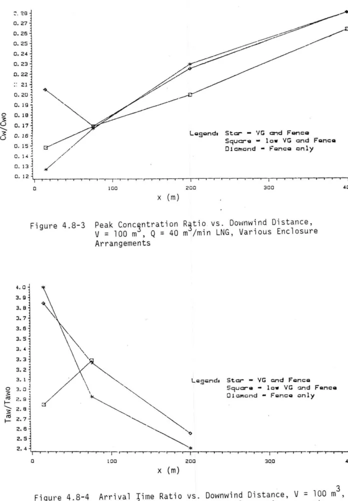
Figure 4.8-3 considers the centerline variation of the peak concentration ratios for the fence· enclosure alone and the two vortex generator additions. Notice that the peak ratio drops to a minimum value at 75 m, but thereafter all cases behave in a similar fashion and increase slowly with downstream distance. Apparently an upwind vortex generator acts to dilute gases before they pass over the downwind fence; hence, the tests with vortex generator installed produced minimum peak concentration ratios at 15 m rather than 75 m.

Figures 4.8-4 to 4.8-6 present arrival time, peak arrival time, and departure time ratios for the same conditions displayed on Figure 4.8-3. Cloud advection times are from 1.5 to 4 times larger than the no enclosure case in the immediate wake of the enclosure;however, by the time the cloud reaches 300 to 400 meters downwind, time ratios are reduced to one or less. This behavior is consistent with that observed for data from the Thorney Island tests discussed in Chapter 4.6.

Given a fence enclosure with a 14.1 m vortex generator upwind of the spill area and an LNG spill rate of 40 cubic meters/min then Figure 4.8-7 presents the influence of increase in total spill volume on peak concentration. Doubling the total spill volume appears to double ground level peak concentrations. Yet an increase in spill volume has less systematic effect on peak arrival time in Figure 4.8-8.

Similarly, Figure 4. 8-9 shows that increasing spill rate while holding spill volume constant may increase peak concentrations, but the

perturbations are much smaller. Increased spill rate produces only minor variations in peak concentration arrival time on Figure 4.8-10.

Figures 4. 8-11 to 4. 8-14 display vertical profiles of concentration, arrival, peak arrival, and departure times for a section 15 m downstream of the downwind enclosure fence. The fence clearly mixes the cloud to greater heights, and a peak in the concentration profile occurs just above fence height (13 m) . The fence also delays the arrival and departure of the cloud in the wake region, but the cloud appears first near fence height.

By the time the cloud reaches 75 m downstream of the fence, the concentrations and arrival, peak arrival, and departure times are essentially constant with height as noted on Figures 4.8-15 to 4.8-18. Measurements at stations farther downstream look similar to the 75 m data sets, except that concentrations are less and times are larger.

Figures 4.8-19 to 4.8-22 and 4.8-23 to 4.8-26 display crosswind profiles of ground level concentrations and cloud times at distance of 15 and 75 m downstream of the fence, respectively. Lateral profiles for the no-enclosure release condition extend to significantly greater lateral distances than the enclosure conditions. Visual observations of the model and field enclosure spills revealed strong three dimensionality in the

cloud. Longitudinal vortices generated at enclosure corners appeared to draw the cloud over the fence first at the corners. Nonetheless, concentrat~on and cloud time data show a strong two-dimensionality in the cloud wake.

Multilinear Regression by ANOVA of Pre-Falcon wind Tunnel Data:

Since the pre-Falcon data set were the most complete, reliable, and comprehensive available, the SAS-PC statistical package was used to estimate coefficients in a multilinear regression on the data. The ANOVA procedure was applied to the logarithmic form of simple power law formula,

i.e.:

(T~/T~₀ - 1) ( II ) ,

(Tp~/TP~o 1) ( II ), and

(Td~/Td~₀ 1) ( II ₎ ,

where subscripts w and wo indicate measurements with and without the enclosure present. The coefficients A, a, b, c, d, and e were determined by the ANOVA procedure. Both Forward, Backward, and Maximizing versions of the multilinear regression procedures were employed. The regression was applied to data from Runs 1, 3, 4, 7, 8, 9, 13, 10, 16, and 17 from the Neff and Meroney data set. Data were always normalized by a no-enclosure reference value taken under the same spill rate and wind speed conditions .

'?.

The regression procedure revealed that inclusion of the Froude number term did not reduce the variance of the prediction equation significantly. This probably occurs because all data points are normalized by data with the same Froude number magnitude. The dominant terms were found to be volume spill rate and total volume spilled. The optimum expressions were determined to be:

(1 - ,Cw/Cwo) (l.S6yo.051*(Vol/Lc3)-0.l63*(H/Lc)0.040*(x/Lc)-o.o35)'

(T~/T~o - 1) (0 .103*y-i.035*(Vol/Lc3)0.sa1*(H/Lc.)o.212*(x/Lc)-o.1a1)'

(Tp~/TP~o - 1) (0. 027*Yo.438*(Vol/Lc 3) 1.2s1*(H/Lc)-o.2s4*(x/Lc)-o.21s)' and

(Td~/Td~₀ - 1) (0. 142*Fr-0· 450* (Vol/Le 3) 0·230* (H/Lc) 1. 332*(x/L_{0 )-}0· 419) . These relations are the best four-variable expressions determinable by the ANOVA approach. Notice the analysis presumes all time ratio data is greater than one and all peak concentration ratio data is less than one. Presuming a correct expression has been derived by the ANOVA procedure the peak concentration ratio formula was used to prepare Figures 4.8-27 and 4.8-28. A range of conditions were selected that might be encountered during an HF release. The first figure predicts peak concentration ratios versus downwind distance for a fixed spili rate and increasing spill volume. The second figure predicts peak concentration ratios versus downwind distance for a fixed spill volume and increasing spill rate. The second figure does not seem physically realistic, since, intuitively, a fence should be very efficient at low 'spill rates. Examination of the original data set reveals that the variations with spill rate are themselves irregular; hence, the unusual behavior in the final regression expression.

Conclusions;

Since each measurement was repeated several times during the pre-Falcon experiment, it is possible to focus on trends that occur with confidence. A fence enclosure around a transient dense gas spill will reduce downwind concentrations, reduce the lateral extent of the cloud near the source, and delay the arrival, peak arrival and departure of the cloud at downwind measurement stations. An increase in total spill volume released or spill rate is expected to increase peak concentrations. Vertical profiles along the plume centerline reveal a maximum in plume concentrations very near the fence, but further downwind the cloud is well mixed in the vertical.

y ·-I Dimensio Field-m Model-c ns _eters

J

entir.ieters 22

l

-- 25

·1

-

-•

•

•

Barrier • ;

Bermed Area _{Spi II Line}

38 x 38\ 112--1 "

-

~ - -.

\

~fl~ ,,,~ - .c )

-"1•\'

'11\'

4tl

~'~

,\t~ - ( )

-'11\'

~T\' - - t

-I_

p _{ent Fence} 88

~.I

Prevailing Wind--+-z 14.1 Vortex Generating Barrier

- -

-~:c__;_ -t---~----~~-1· _;~ -=:_~=--~--~~~-~~ ~:--

--

~~----{~

--

--1:---F=-~L.:..~~Ji---~---_;: ___ -.fl T 1 ti = :• 11 • '• ' 1 ii 11 tt ~ II : II Ii ~ u 9 4 - - -~l- --

-t--

-;~-

-,

i~

-::-+----:;--:;---{---

~:- ----~r--- -~----+---~---ri---~---!:---- · ·: !. ~ !• :, ( ~: •• ~ ~~ ·: .. ~ _}.. ~ ~ ) ..

Tube Battens Fiber Re in forced Fobr ic Pipe Support

Figure

4~8-1

Fence Enclosure Geometry,

Pre-F~lcon

Wind-tunnel Tests

Vo rte)( Generating Barrier. Vapor Fence1 ' y

•

•

•

•

• •

•

Measurement Separation

•

• •

• •

_•

•

•

• •

•

• •

Distonc~

9

in

y Dimensions Field - meters Model - centimeters

•

_•

•

•

•

_•

• •

•

•

_•

•

•

•

•

x

.

•

---• ---•

• •

• •

•

• •

•

• •

•

0 15 75 200 400

Figure 4.8-2

x

Measurement Grid, Pre-Falcon Wind-tunnel Tests

0 20 40 60 y 80 100 120 140

0 3 u ... 3 u :' . ~8 a. 27 0.26 0.25 o. 24 D. 23 0.22 :: 21 l o. 201

~:

_a.

:: l

17 D. 15 0. 15

~

~ 0. l 4 ~ o. l3

i

a. 12

"'

"'

/ /

/

I I I I I / I --r--T"

Lg9gnd1 Stor - VG end FcancQ

Sgucrg • low VG and Fgnca

Dic~cnd • Fgncg only 0 100 200 300 400 4. a 3. 9 3. 8 J. 7 3.6 x ( m)

Figure 4.8-3 Peak

Conc~ntration R~tio

vs. Downwind Distance,

V

=

100 m ,

Q

=

40 m /min LNG, Various Enclosure

a

Arrangements

100

x (m) 200

Ster - VG ond Fgncg

S9uore • lo• VG and Fanca 0101nond • Fgnca only

300 ~oa

Figure

4.8-4

Arrival 1ime Ratio vs . Downwind Distance,

V

=

100

m

3

,

Q

=

40 m /min LNG, Various Enclosure Arrangements

2.

41

2. 3 2.2 2. l 2. a 1. g 1. 8 l. 7 0 3 I. 5 .. 0.. ... _{1. 5} ... 3 0. 1. 4 ... 1. 3 1. 2 1. 1 1. a 1.

61

1. 5 1.

"1·

1. 3

~

_~~

\ ~

Li;iggnda Star - '/G and Fgncg

Ssuorg - low VG end FQncQ O!omond • Fgncg o~ly

i._-~~~~~---.---.---..--._,r--r--..-r-r-r ·

·-a 100 200 JOO

X ( m)

Figure 4.8-5 Peak

Arri~al

Time Ra3io vs. Downwind Distance,

V

=

100 m ,

Q

=

40 m /min LNG, Various Enclosure

Arrangements

~1.21'

.> if'~

~ i /

Star • VG and Fgncg

S9worg • lov VG end FgncQ

D1~~ond - F~ncQ only

!:::1,

r.f'"' o. 9

j

'

""

_~

' O.B\-r-r-r-r--r-r--r-'T"""""r-T"--.--.-...-.-.---.-~~~~~ ~ ~,-a

Figure 4.8-6

100 200 3CO

x

(m)

Departur3 Time Ratio vs. Downwind Distance, V

=

100

Q

=

40 m /min LNG, Various Enclosure Arrangements

99

4CO

400

3

-

~'? 3: u u <V (/) 0. f-10 g a 71 , 6 s

..

31

21 1 ] l j Lc9Qnd1 Star - Val - 100 cu ~ Squqr-Q - Vol - 70 cu M 81c~ond - Vol - SO cu •

-=---

_-~ ~ a 320

j

3101

300

l

290 2ao 27C

1

260 250 240 230 220

j

210 200 100 2CO 300 X ( m)

Figure 4.8-7 Peak Concentration vs. Downwind

Dist~nce,

14. 1 m

Vortex Generator and Fence,

Q

=

40 m /min LNG,

Various Total Spill Volumes

>If

\

\

_/

/ /

/

~~

L~gur. (..;, Ster - '/ol • lCO C\J .,

S9uara - './al - 70 cu "'

C:~~cnd - Vcl - 50 cu m

T--r · -i-1--·T--r-·-r--r--r-r·-..,-·-,.-..--r-r-.,--,.--,--..-~..,~

lCO 2Cu 300

X (m)

Figure 4.8-8 Arrival Time vs. Downwind

Dis~ance,

14. l m Vortex

Generator and Fence,

Q

=

40 m /min LNG, Various

Total Spill Volumes

100