Abstract— The main purpose of this study was to determine whether it is possible to somehow use results on training or validation data to estimate ensemble performance on novel data. With the specific setup evaluated; i.e. using ensembles built from a pool of independently trained neural networks and targeting diversity only implicitly, the answer is a resounding no. Experimentation, using 13 UCI datasets, shows that there is in general nothing to gain in performance on novel data by choosing an ensemble based on any of the training measures evaluated here. This is despite the fact that the measures evaluated include all the most frequently used; i.e. ensemble training and validation accuracy, base classifier training and validation accuracy, ensemble training and validation AUC and two diversity measures. The main reason is that all ensembles tend to have quite similar performance, unless we deliberately lower the accuracy of the base classifiers. The key consequence is, of course, that a data miner can do no better than picking an ensemble at random. In addition, the results indicate that it is futile to look for an algorithm aimed at optimizing ensemble performance by somehow selecting a subset of available base classifiers.
I. INTRODUCTION
lthough the use of Artificial Neural Networks (ANNs) will most often lead to very accurate models, it is also well known that even higher accuracy can be obtained by combining several individual models into ensembles; see e.g. [1] and [2].
An ensemble is a composite model aggregating multiple base models, making the ensemble prediction a function of all included base models. Ensemble learning, consequently, refers to methods where a target function is learnt by training and combining a number of individual models.
The main reason for the increased accuracy obtained by ensembles is the fact that uncorrelated base classifier errors will be eliminated when combining several models using averaging; see e.g. [3]. Naturally, this requires the base classifiers to commit their errors on different instances – there is nothing to gain by combining identical models. Informally, the key term diversity therefore means that the base classifiers make their mistakes on different instances.
While the use of ensembles is claimed to virtually guarantee increased accuracy compared to the use of single models, the problem of how to maximize ensemble accuracy is far from solved. In particular, the relationship between
U. Johansson and T. Löfström are equal contributors to this paper. U. Johansson and T. Löfström are affiliated with the School of Business and Informatics, University of Borås, SE-501 90 Borås, Sweden. Email: {ulf.johansson, tuve.lofstrom}@hb.se
H. Boström is affiliated with the School of Humanities and Informatics, University of Skövde, Sweden. Email: henrik.bostrom@his.se
ensemble diversity and accuracy is not completely understood, making it hard to efficiently utilize diversity for ensemble creation.
The very important result that ensemble error depends not only on the average accuracy of the base models but also on their diversity was formally derived in [4]. Based on this, the overall goal when creating an ensemble seems to be to combine models that are highly accurate, but differ in their predictions. Unfortunately, base classifier accuracy and diversity are highly correlated, so maximizing diversity would most likely reduce the average accuracy. In addition, diversity is not uniquely defined for predictive classification. Because of this, several different diversity measures have been suggested, and, to further complicate matters, no specific diversity measure has shown high correlation with accuracy on novel data.
It should be noted that even though performance of predictive classification models are normally evaluated using accuracy, there is an alternative metric frequently used called area under the ROC curve (AUC). Accuracy is the proportion of instances classified correctly when the model is applied to novel data; i.e. it is based only on the final classification. AUC, on the other hand, measures the model’s ability to rank instances based on how likely they are to belong to a certain class. AUC can, more specifically, be interpreted as the probability of an instance that do belong to the class being ranked ahead of an example that do not belong to the class; see e.g. [5].
The purpose of this study is to look into ensemble member selection based on performance on training or validation data. More specifically, the assumption is that we have a number of individually trained ANNs, and the task is to select a subset of these to form an ensemble. Naturally, what we would like to maximize are ensemble accuracy and ensemble AUC, when applying the ensemble to novel (test) data. The performance measures available on training and/or validation data are base classifier accuracy, ensemble accuracy, ensemble AUC and numerous diversity measures.
II. BACKGROUND AND RELATED WORK
As mentioned above, Krogh and Vedelsby, in [4], derived an equation stating that the generalization ability of an ensemble is determined by the average generalization ability and the average diversity (ambiguity) of the individual models in the ensemble. More specifically; the ensemble error, E, can be calculated using
E=E− (1) A
The Problem with Ranking Ensembles Based on
Training or Validation Performance
Ulf Johansson, Tuve Löfström and Henrik Boström
where E is the average error of the base models andAis the ensemble diversity, measured as the weighted average of the squared differences in the predictions of the base models and the ensemble. In a regression context and using averaging, this is equivalent to:
2 1 2 1 2 ˆ ˆ ˆ ˆ ( ens ) ( i ) ( i ens) i i E Y Y Y Y Y Y M M = − =
¦
− −¦
− (2)The first term is the (possibly weighted) average of the individual classifiers and the second is the diversity term; i.e. the amount of variability among ensemble members. Since diversity is always positive, this decomposition proves that the ensemble will always have higher accuracy than the average accuracy obtained by the individual classifiers. The problem is, however, the fact that the two terms are normally highly correlated, making it necessary to balance them rather than just maximizing diversity.
For classification, where a zero-one loss function is used, it is, however, not possible to decompose the ensemble error into error rates of the individual classifiers and a diversity term. Instead, algorithms for ensemble creation typically use heuristic expressions trying to approximate the unknown diversity term. Naturally, the goal is to find a diversity measure highly correlated with majority vote accuracy.
The most renowned ensemble techniques are probably bagging [6], boosting [7] and stacking [8], all of which can be applied to different types of models, and used for both regression and classification. Most importantly; bagging, boosting and stacking will, almost always, increase predictive performance compared to a single model. Unfortunately, machine learning researchers have struggled to understand why these techniques work; see e.g. [9]. In addition, it should be noted that these general techniques must be regarded as schemes rather than actual algorithms, since they all require several design choices and parameter settings.
Brown et al. [10] introduced a taxonomy of methods for creating diversity. The first obvious distinction made is between explicit methods, where some metric of diversity is directly optimized and implicit methods, where the method is likely to produce diversity without actually targeting it. After that Brown et al. move on to group methods using three categories; starting point in hypothesis space, set of accessible hypotheses and traversal of hypothesis space. These categories, and how they apply to ANN ensembles, are further described below.
For ANNs, the most obvious method for choosing a starting point in hypothesis space is to simply randomize the initial weights; something that must be considered a standard procedure for all ANN training. Alternatively, the weights could be deliberately initialized to different parts of the hypothesis space. Unfortunately, experimentation has found that ANNs often converge to the same, or very similar optima, in spite of starting in different parts of the space; see e.g. [11]. Thus, according to Brown et al., varying the initial weights of ANNs does not seem to be an effective
stand-alone method for generating diversity.
The two main principles regarding set of accessible hypotheses are to manipulate either training data or the architecture. Several methods attempt to produce diversity by supplying each classifier with a slightly different training set. Regarding resampling, the view is that it is more effective to divide training data by feature than by pattern; see [12]. All standard resampling techniques are by nature implicit. The well-known technique AdaBoost [13], on the other hand, explicitly alters the distribution of training data fed to each classifier based on how “hard” each pattern is.
Manipulation of architectures is, for ANNs, most often about number of hidden units, something that, according to Brown et al., also turns out to be quite unsuccessful. Hybrid ensembles where, for instance, MLPs and RBF networks are combined, are sometimes considered to be a “productive route”; see [14]. Regarding hybrid ensembles, Brown et al. argue that two systems representing the problem and search the space in very different ways probably will specialize on different parts of the search space. This implies that when using hybrid ensembles, it could possibly be better to select one specific classifier instead of combining outputs.
A common solution for traversal of hypothesis space is to use a penalty term enforcing diversity in the error function when training ANNs. A specific, and very interesting example, is Negative Correlation learning (NC) [15], where the covariance between networks is explicitly minimized. For regression problems it has been shown that NC directly controls the covariance term in the bias-variance-covariance trade-off; see [16]. For classification problems, however, this does not apply since the outputs have no intrinsic ordinality between them, thus making the concept of covariance undefined.
Finally, Brown et al. discuss evolutionary methods where diversity is a part of a fitness function and some evolutionary algorithm is used to search for an accurate ensemble. One example is the ADDEMUP method, presented in [17].
Unfortunately, several studies have shown that all diversity measures evaluated show low or very low correlation with ensemble accuracy; see e.g. [18] and [19]. In addition, our last study [19] also showed that correlations between training or validation accuracies and test accuracies almost always were remarkably low. The main reason for this apparent anomaly is that when ensembles are evaluated, most ensembles tend to have very similar training or validation accuracy. Furthermore, validation sets are often rather small, so confidence intervals for true error rates when estimated using validation data become quite large.
More formally, when using a validation set to estimate the true error rate, the only information available is the number of errors e on the validation set of size N. The correctness when classifying a novel instance (from the validation set) can be regarded as a random variable with a Bernoulli distribution. The number of errors, Y, on a validation set of size N, thus is a sum of Bernoulli distributed random
variables, making Y a random variable with a binomial distribution. The sample error Y = e/N, is an unbiased estimator for the true error rate p. The variance for e is Np(1-p), where p has to be substituted with the estimator e/N. Since the parameters for the binomial distribution governing the sample error are known, a confidence interval for p is established by finding the interval centered around the sample error holding an appropriate amount (e.g. 95%) of the total probability under this distribution. Normally, this calculation is not performed directly; i.e. actually using the binomial distribution. The standard procedure is instead to use the normal distribution as an approximation; leading to the confidence interval for p given in equation (3) below.
/ 2 (1 ) (1 ) e e e N N p Z N α N
α
− = ± − (3)As an example, if the Bupa liver disorders data set from UCI repository is used, the total number of instances is 345. Assuming an apparent error rate of 0.35, and that 70% of the instances were used for training, 20% for validation and 10% for testing, the confidence interval for p using α=0.05 is 0.35±0.11; i.e. the corresponding accuracy is between 0.54 and 0.76. Consequently, when most ensembles obtain similar validation accuracies - which is the normal situation - their confidence intervals for true error rates will be highly overlapping. Exactly how this reasoning applies to using diversity measures as estimators is not obvious. Experimentation shows, however, that in practice, correlations between diversity measures and test accuracies are even lower than correlations between validation accuracies and test accuracies; see e.g. [19].
Clearly, these results are very discouraging, making it extremely hard to suggest a training or validation measure to use for optimizing ensembles. Possibly, however, the results could, at least to some degree, be due to the use of correlation as criterion. We argue that the main issue is whether an ensemble ranked ahead of another on some training or validation measure retains this advantage on test accuracy or test AUC. With this in mind, the overall purpose of this study is to investigate how well ensemble rankings produced from different training and validation measures agree with test accuracy and test AUC.
III. METHOD
The most important purpose of this study is to evaluate measures on training or validation data that could be used to estimate ensemble performance on novel (test) data. Ensemble performance is here either ensemble accuracy or ensemble AUC. More specifically, we intend to investigate altogether five measures: accuracy, base classifier accuracy, AUC, and the diversity measures double-fault and difficulty. Accuracy is the accuracy of the ensemble on training or validation data. Base classifier accuracy is the average accuracy obtained by the base classifiers on training or
validation data. AUC is the AUC obtained by the ensemble on training or validation data.
If the output of each classifier Di is represented as an
N-dimensional binary vector yi,where the jth element yj,i=1 if
Di recognizes correctly instance zj and 0 otherwise, a
description of pair-wise diversity measure, where the notation Nab refers to the number of instances for which yj,i=a and yj,k=b, is often used. As an example, N11 is the
number of instances correctly classified by both classifiers. Using this notation, the double-fault diversity measure, which is the proportion of instances misclassified by both classifiers, is defined as 00 , 11 10 01 00 i k N DF N N N N = + + + (4) For an ensemble consisting of L classifiers, the averaged double-fault (DF) over all pairs of classifiers is
1 , 1 1 2 ( 1) L L av i k i k i DF DF L L − = = + = −
¦ ¦
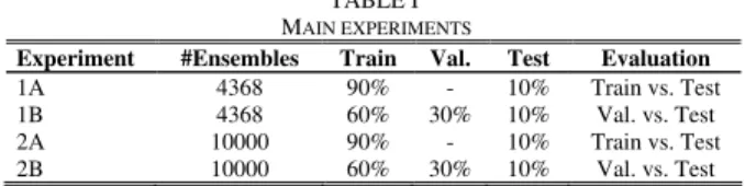
(5) The difficulty measure was used in [20] by Hanson and Salomon. Let X be a random variable taking values in {0/L, 1/L,…, L/L}. X is defined as the proportion of classifiers that correctly classify an instance x drawn randomly from the data set. To estimate X, all L classifiers are run on the data set. The difficulty ș is then defined as the variance of X. The reason for including only these two diversity measures is simply the fact that they have performed slightly better in previous studies; see [19].The empirical study is divided in two main experiments, each consisting of two parts. In the first experiment, 16 ANNs are trained and all 4368 possible ensembles consisting of exactly 11 ANNs are evaluated. In the second experiment, a total of 16 ANNs are trained and then 10000 different ensembles are formed from this pool of ANNs. Here, each ensemble consists of a random subset of the available ANNs. Both experiments are divided in two parts, the difference being whether an extra validation set is used or not. If no validation set is used, all measures and ranking are on the training set. When a validation set is used, this set is not used at all during ANN training, but all measures and rankings are obtained using the validation set. For actual experimentation, 10-fold stratified cross-validation is used. The experiments are summarized in Table I below.
TABLE I MAIN EXPERIMENTS
Experiment #Ensembles Train Val. Test Evaluation
1A 4368 90% - 10% Train vs. Test
1B 4368 60% 30% 10% Val. vs. Test
2A 10000 90% - 10% Train vs. Test
2B 10000 60% 30% 10% Val. vs. Test
A. Ensemble settings
All ANNs used in the experiments are fully connected feed-forward networks. In each experiment, ½ have one hidden layer and the remaining ½ have two hidden layers. The exact
number of units in each hidden layer is slightly randomized, but is based on the number of inputs and classes in the current data set. For an ANN with one hidden layer the number of hidden units is determined from (6) below.
2 ( )
h
¡
¡
¢
rand¸ v c¸°
°
±
(6) Here, v is the number of input variables and c is the number of classes. rand is a random number in the interval [0, 1]. For ANNs with two hidden layers, the number of units in the first and second hidden layers are h1 and h2, respectively.1 ( ) / 2 4 ( ( ) / )
h
¡
¡
¢
v c¸ rand¸ v c¸ c°
°
±
(7)2 ( ( ) / )
h
¡
¡
¢
rand¸ v c¸ c c°
°
±
(8) The diversity is obtained by using ANNs with different architectures, as described above. Furthermore, only 90% (or at most all but one) of the features (randomly selected) are used for training of each net. Majority voting is used to determine ensemble classifications.In Experiment 1, all possible ensembles of size 11 out of 16 are evaluated. In the second experiment, 10000 ensembles, each consisting of a random subset from the 16 available ANNs, are used. It is ensured that no duplicates, and no ensembles with less than 7 ANNs are used. Consequently, the ensembles in the second experiment consist of between 7 and 15 ANNs.
B. Data sets
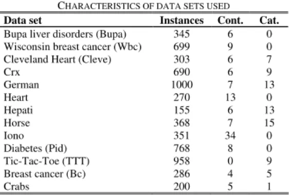
The 13 data sets used are all publicly available from the UCI Repository [21]. For a summary of the characteristics of the data sets, see Table III. Instances is the total number of instances in the data set. Classes is the number of output classes in the data set. Cont. is the number of continuous input variables and Cat. is the number of categorical input variables.
TABLE II
CHARACTERISTICS OF DATA SETS USED
Data set Instances Cont. Cat.
Bupa liver disorders (Bupa) 345 6 0 Wisconsin breast cancer (Wbc) 699 9 0
Cleveland Heart (Cleve) 303 6 7
Crx 690 6 9 German 1000 7 13 Heart 270 13 0 Hepati 155 6 13 Horse 368 7 15 Iono 351 34 0 Diabetes (Pid) 768 8 0 Tic-Tac-Toe (TTT) 958 0 9 Breast cancer (Bc) 286 4 5 Crabs 200 5 1 IV. RESULTS
When presenting the results, we start by showing correlations between the evaluated measures and test set performance. Tables III below shows the results for Experiment 1A; i.e. the measures are evaluated on training
data and using enumerated ensembles. The values tabulated in the first five columns are correlations between the specific measure and test set accuracy. Similarly, the next five columns show correlations between the specific measure and test set AUC. It is, of course, slightly dubious to average correlations, but it was deemed to be the most straightforward way to report these results. The last three columns, finally, show the minimum, maximum and average test set accuracies obtained by the ensembles used for the evaluation. It should be noted that in order to make the tables more readable, the correlations reported are for DF and DIF between high diversity and high performance.
TABLE III
EXPERIMENT 1A –CORRELATION BETWEEN MEASURES ON TRAINING SET AND TEST SET PERFORMANCE.ENUMERATED ENSEMBLES
Corr. with Accuracy Corr. with AUC Accuracy Dataset Acc AUC BAcc DF DIF Acc AUC BAcc DF DIF Min Max Avg
Bupa -.15 -.04 -.05 -.02 -.01 -.20 -.10 -.05 -.11 -.11 .62 .79 .71 Wbc .01 .01 -.05 -.04 -.04 -.10 -.14 -.18 -.18 -.19 .95 .97 .96 Cleve -.08 -.08 -.08 -.09 -.09 -.14 -.17 -.24 -.22 -.22 .75 .88 .82 Crx .09 .08 .09 .11 .09 .03 .06 .05 .08 .05 .84 .90 .87 German -.05 -.03 -.06 -.05 -.05 -.17 -.18 -.14 -.15 -.15 .71 .81 .76 Heart -.15 -.12 -.12 -.14 -.13 -.04 .00 -.11 -.05 -.06 .75 .89 .82 Hepati .01 .00 -.06 -.03 -.05 .01 .00 .07 .06 .07 .77 .89 .84 Horse .03 .03 .07 .07 .07 .04 .02 .13 .10 .11 .76 .88 .82 Iono .03 .00 .04 .04 .06 .04 .00 .08 .04 .06 .90 .96 .93 Pid -.09 -.14 -.13 -.13 -.10 -.02 .00 .00 .00 .01 .73 .81 .77 TTT .43 .43 .39 .43 .44 .56 .66 .50 .57 .59 .81 .93 .88 Bc .07 .02 .04 .04 .04 .04 -.01 .00 .05 .06 .63 .80 .73 Crabs .01 .08 .07 .07 .07 .00 .03 -.01 -.01 -.01 .91 .98 .96 MEAN .01 .02 .01 .02 .02 .00 .01 .01 .01 .02 .78 .88 .84
With the exception of the Tic-Tac-Toe dataset, all correlations are very low to non-existent. On some data sets, like Bupa, Cleve and German, all correlations are in fact negative; i.e. less diverse ensembles, with lower training accuracy, lower training AUC, and lower base classifier training accuracy actually obtained higher test set accuracies and AUCs! At the same time, it should be noted that, as seen in the last three columns, for most datasets there is at least some spread in ensemble performance. So, based on these results, it appears to be obvious that none of the measures can be used as a sole criterion for optimizing ensemble test set accuracy or AUC. The results of Experiment 1B; i.e. using a separate validation set and enumerated ensembles are shown in Table IV below.
TABLE IV
EXPERIMENT 1B–CORRELATION BETWEEN MEASURES ON VALIDATION SET AND TEST SET PERFORMANCE.ENUMERATED ENSEMBLES
Corr. with Accuracy Corr. with AUC Accuracy Dataset Acc AUC BAcc DF DIF Acc AUC BAcc DF DIF Min Max Avg
bupa .03 .07 .10 -.01 -.09 .13 .10 .10 .12 .00 .63 .79 .71 wbc .02 .05 .05 .03 .03 .02 .06 -.04 .01 .02 .96 .98 .97 cleve .01 .03 .08 .01 -.06 .00 .07 .06 .06 .02 .72 .88 .81 crx .02 .01 .07 .03 -.03 .08 .22 .18 .08 -.08 .81 .89 .85 german .09 .05 .16 .09 -.05 .08 .20 .21 .12 -.03 .69 .82 .75 heart .04 .02 -.01 .04 .06 .07 .11 .08 .07 .05 .73 .88 .82 hepati -.01 .01 .02 -.01 -.03 .08 -.02 -.04 .04 .08 .77 .90 .85 horse .07 .09 .18 .08 -.03 .01 .02 .12 .08 -.04 .73 .88 .82 iono .00 .03 -.05 -.01 .01 .06 .08 .11 .09 .09 .88 .95 .92 pid .12 .08 .06 .14 .06 .12 .16 .22 .02 -.13 .72 .81 .77 TTT .42 .45 .49 .52 .47 .40 .58 .51 .57 .53 .78 .91 .86 Bc .02 -.04 -.02 -.02 -.01 -.09 -.14 -.12 -.06 .01 .63 .80 .71 crabs .10 .04 .13 .11 .06 .00 .05 -.02 -.01 -.02 .89 .96 .92 MEAN .07 .07 .10 .08 .03 .07 .11 .10 .09 .04 .76 .88 .83
Here, the results are very similar, although not quite as extreme. Now it is at least almost always positive to have a high validation accuracy or AUC. Still, the level of correlations makes it extremely unlikely that using one of the measures as selection criteria would actually be beneficial compared to just picking one ensemble at random. Tables V and VI below show the results from Experiments 2A and 2B; i.e. when using randomized ensembles.
TABLE V
EXPERIMENT 2A–CORRELATION BETWEEN MEASURES ON TRAINING SET AND TEST SET PERFORMANCE.RANDOM ENSEMBLES
Corr. with Accuracy Corr. with AUC Accuracy Dataset Acc AUC BAcc DF DIF Acc AUC BAcc DF DIF Min Max Avg
bupa -.17 -.06 -.06 -.06 .00 -.20 -.07 -.02 -.10 -.05 .59 .80 .71 wbc .00 .00 -.08 -.06 -.05 -.11 -.11 -.18 -.18 -.17 .94 .98 .96 cleve -.07 -.05 -.08 -.08 -.07 -.17 -.14 -.24 -.22 -.21 .72 .90 .82 crx .10 .08 .12 .10 .09 .08 .09 .07 .09 .09 .81 .91 .87 german -.03 .01 -.04 -.04 -.01 -.15 -.12 -.14 -.16 -.11 .69 .82 .76 heart -.13 -.08 -.12 -.13 -.12 -.04 .01 -.13 -.06 -.05 .70 .92 .82 hepati .01 .00 -.06 -.02 -.04 .00 .00 .07 .06 .08 .73 .95 .84 horse .01 .03 .06 .05 .06 .07 .05 .12 .10 .14 .73 .91 .82 iono .02 .00 .02 .01 .04 .06 .02 .08 .04 .08 .88 .97 .93 pid -.08 -.10 -.08 -.12 -.10 -.01 .01 .00 -.01 .03 .71 .82 .77 TTT .51 .50 .45 .49 .52 .59 .69 .49 .56 .63 .76 .94 .87 Bc .03 .03 .01 .01 .03 .05 .01 .01 .06 .08 .60 .82 .73 crabs .09 .18 .15 .17 .17 .08 .15 .05 .07 .07 .87 .99 .95 MEAN .02 .04 .02 .03 .04 .02 .04 .01 .02 .05 .75 .90 .83 TABLE VI
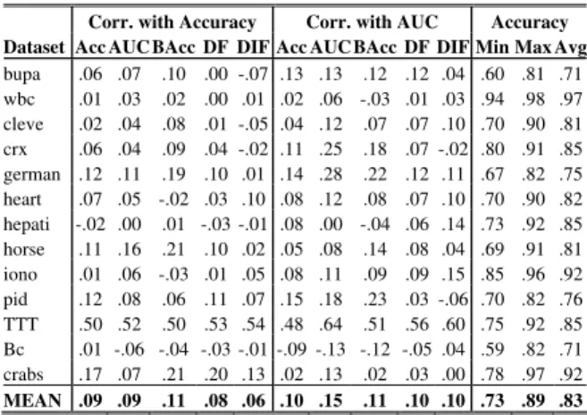
EXPERIMENT 2B–CORRELATION BETWEEN MEASURES ON VALIDATION SET AND TEST SET PERFORMANCE.RANDOM ENSEMBLES
Corr. with Accuracy Corr. with AUC Accuracy Dataset Acc AUC BAcc DF DIF Acc AUC BAcc DF DIF Min Max Avg
bupa .06 .07 .10 .00 -.07 .13 .13 .12 .12 .04 .60 .81 .71 wbc .01 .03 .02 .00 .01 .02 .06 -.03 .01 .03 .94 .98 .97 cleve .02 .04 .08 .01 -.05 .04 .12 .07 .07 .10 .70 .90 .81 crx .06 .04 .09 .04 -.02 .11 .25 .18 .07 -.02 .80 .91 .85 german .12 .11 .19 .10 .01 .14 .28 .22 .12 .11 .67 .82 .75 heart .07 .05 -.02 .03 .10 .08 .12 .08 .07 .10 .70 .90 .82 hepati -.02 .00 .01 -.03 -.01 .08 .00 -.04 .06 .14 .73 .92 .85 horse .11 .16 .21 .10 .02 .05 .08 .14 .08 .04 .69 .91 .81 iono .01 .06 -.03 .01 .05 .08 .11 .09 .09 .15 .85 .96 .92 pid .12 .08 .06 .11 .07 .15 .18 .23 .03 -.06 .70 .82 .76 TTT .50 .52 .50 .53 .54 .48 .64 .51 .56 .60 .75 .92 .85 Bc .01 -.06 -.04 -.03 -.01 -.09 -.13 -.12 -.05 .04 .59 .82 .71 crabs .17 .07 .21 .20 .13 .02 .13 .02 .03 .00 .78 .97 .92 MEAN .09 .09 .11 .08 .06 .10 .15 .11 .10 .10 .73 .89 .83
The overall results here are again quite similar to the first experiment. The main reason for the slightly higher values overall is probably that some ensembles in this experiment have significantly lower accuracy; see the Min column. This is an interesting, but discouraging result. It appears like the only way to increase the benefit of using the investigated measures when selecting an ensemble, is to make sure that some ensembles perform poorly.
As mentioned above, it could be argued that correlation over the entire data set is not really the most important criterion. After all, we would eventually have to choose one ensemble to apply on unseen data. So, the interesting question is instead whether an ensemble with better performance on training or validation data will keep this edge when applied to test data. To emulate this, we for each experiment and measure, divided the ensembles in three groups, based on training or validation performance. As an example, for Experiment 1A (enumerated ensembles and using training data), the ensembles were sorted using each measure; i.e. training accuracy, training DF etc. Then, the ensembles were split in three equally sized parts; where Group 1 is the third of the ensembles with the lowest training performance and Group 3 is the third with highest performance. Finally, the three groups were pair-wise compared using test accuracy. More specifically, when comparing, for instance Group 1 and Group 2, each ensemble in Group 1 was compared to every ensemble in Group 2. Using this scheme, the results reported below are the percentages of wins for each group. As an example, the first pair of numbers in Table VII below (26.3% / 27.9%) is from the comparison of the worst group with the middle group; measured using ensemble training accuracy. The numbers say that Group 1 won 26.3% (of the test set accuracy matches) and Group 2 won 27.9%. Consequently 45.8% of all matches were ties.
TABLE VII
EXPERIMENT 1A – ENUMERATED ENSEMBLES, TRAIN-TEST
1 vs 2 2 vs 3 1 vs 3 Acc 26.3% / 27.9% 26.7% / 27.2% 26.7% / 28.6% AUC 25.8% / 28.3% 27.3% / 26.5% 26.9% / 28.6% BAc 26.3% / 28.0% 26.9% / 26.6% 26.9% / 28.2% DF 26.9% / 26.7% 25.9% / 28.2% 26.7% / 28.7% DIF 26.4% / 27.2% 26.1% / 28.1% 26.5% / 29.0% TABLE VIII
EXPERIMENT 1B – ENUMERATED ENSEMBLES, VAL-TEST
1 vs 2 2 vs 3 1 vs 3 Acc 27.1% / 31.9% 27.3% / 30.7% 26.0% / 33.8% AUC 26.8% / 31.8% 27.3% / 31.4% 25.7% / 34.4% BAc 26.0% / 32.8% 26.2% / 32.2% 24.5% / 36.2% DF 26.8% / 31.4% 26.6% / 32.2% 25.5% / 34.9% DIF 28.3% / 30.4% 28.4% / 30.3% 28.4% / 31.9% TABLE IX
EXPERIMENT 2A – RANDOM ENSEMBLES, TRAIN-TEST
1 vs 2 2 vs 3 1 vs 3 Acc 29.1% / 31.6% 29.6% / 30.2% 29.8% / 32.1% AUC 28.8% / 32.2% 29.3% / 30.3% 29.1% / 32.9% BAc 28.3% / 31.8% 30.4% / 29.3% 30.1% / 32.2% DF 30.5% / 29.7% 28.3% / 31.4% 30.3% / 32.1% DIF 29.5% / 30.0% 28.3% / 32.1% 29.3% / 33.0% TABLE X
EXPERIMENT 2B – RANDOM ENSEMBLES, VAL-TEST
1 vs 2 2 vs 3 1 vs 3 Acc 27.8% / 34.8% 28.4% / 32.5% 26.6% / 37.0% AUC 27.6% / 34.7% 28.8% / 32.5% 26.8% / 36.9% BAc 26.7% / 35.4% 28.2% / 33.0% 26.1% / 38.2% DF 29.1% / 32.3% 27.6% / 34.5% 27.4% / 36.7% DIF 29.1% / 31.7% 29.3% / 33.4% 28.7% / 35.0%
The results presented in Tables VII-X above basically suggest two things. The first and most obvious is that many ensembles get exactly the same test set accuracies. In fact, the number of ties is always more than one third of all matches. The second observation is that the difference in wins between two groups generally is very low. As expected, the differences are slightly larger between the best and worst group, especially when using random ensembles and a validation set, but it is still almost marginal. In summary, the tables above show that the benefit of using any of the evaluated measures to rank ensembles turned out to be very small in practice.
Having said that, Figure 1 and Figure 2 below give a slightly different picture. These figures illustrate how ensembles sorted on training or validation measures perform on a test set. In both figures, all ensembles are grouped into ten groups, and the test set results are average results for all ensembles in that group. It should be noted that in these figures the results over all datasets are aggregated without adjusting for the different levels.
1 2 3 4 5 6 7 8 9 10 0.666 0.667 0.668 0.669 0.67 0.671 0.672 0.673 0.674 Acc AUC BAcc DF DIF Figure 1: Experiment 2A – Performance on test set. Accuracy
1 2 3 4 5 6 7 8 9 10 0.705 0.706 0.707 0.708 0.709 0.71 0.711 0.712 Acc AUC BAcc DF DIF Figure 2: Experiment 2A – Performance on test set. AUC
The Y-axis is test set accuracy (Figure 1) and test set AUC (Figure 2), respectively. The points on the X-axis are the ten groups. The ensembles with best performance on training data belong to the tenth group, and those with worst performance belong to the first. Again, it is evident that the difference between ensembles with poor training performance and those with better training performance is very low. The difference in average test set accuracy, between Group 1 and Group 10, when the ranking is based on base classifier training accuracy is about 0.005, and for the other measures, it is even less. The same pattern is evident in Figure 2 as well. Nevertheless, the rising curves indicate that it may still be slightly beneficial to use ensembles with better training or validation performance. Exactly how to select one ensemble, more likely than another to perform well on novel data remains, however, a very difficult question.
V. CONCLUSIONS
The main purpose of this study was to determine whether it is possible to somehow use results on training or validation data to estimate ensemble performance on novel data. With the specific setup evaluated; i.e. using ensembles built from a pool of independently trained ANN, and targeting diversity only implicitly, the answer is a resounding no. It should be noted that the measures evaluated include all the most frequently used; i.e. ensemble training and validation accuracy, base classifier training and validation accuracy, ensemble training and validation AUC and diversity measured as double fault or difficulty. Despite this, the results clearly show that there is in general nothing to gain, in performance on novel data, by choosing an ensemble based on any of these measures. Experimentation shows not only that correlations between available training or validation measures and test set performance are very low, but also that there is no indication on that ensembles with better performance on training or validation data will keep this edge on test data. So, the overall conclusion is that none of the measures evaluated is a good predictor for ensemble test set performance.
VI. DISCUSSION AND FUTURE WORK
First of all, it is important to realize that these results do not challenge ensembles in general. There is overwhelming evidence, both theoretical and empirical, that ensembles will outperform single models. In addition, this study does not suggest that implicit diversity is not beneficial. Quite the contrary, diverse ensembles will normally outperform homogenous, and implicit diversity is the easiest way to accomplish that. The main conclusion of this study is instead that, given the specific setup, it is not possible for a data miner to use any measure available on training or validation data, to make an informed guess which ensemble to apply on unseen data.
It could be argued that the results are partly due to the rather small datasets and the use of 10-fold cross-validation, which make test sets very small. This is a relevant objection, and it is obvious that the setup used leads to a lot of ensembles having very similar performance. Still, that is precisely the point. Unless we deliberately try to create less accurate base classifiers, we will get exactly this situation. Preliminary experiments using larger datasets and 4-fold cross-validation instead, also show that this problem prevails.
ACKNOWLEDGMENT
This work was supported by the Information Fusion Research Program (University of Skövde, Sweden) in partnership with the Swedish Knowledge Foundation under grant 2003/0104 (URL: http://www.infofusion.se).
REFERENCES
[1] T. G. Dietterich, Ensemble Methods in Machine Learning, 1st
International Workshop on Multiple Classifier Systems, Cagliari,
Italy, Springer-Verlag, LNCS 1857:1-15, 2000.
[2] D. Opitz and R. Maclin, Popular ensemble methods: an empirical study, Journal of Artificial Intelligence Research, 11:169-198, 1999. [3] T. G. Dietterich, Machine learning research: four current directions,
The AI Magazine, 18: 97-136, 1997.
[4] A. Krogh and J. Vedelsby, Neural network ensembles, cross validation, and active learning. Advances in Neural Information
Processing Systems, Volume 2: 650-659, San Mateo, CA, Morgan
Kaufmann, 1995.
[5] T. Fawcett, Using rule sets to maximize roc performance, 15th
International Conference on Machine Learning, pp. 445-453, 2001.
[6] L. Breiman. Bagging predictors, Machine Learning, 24(2), pp. 123-140, 1996.
[7] Shapire, R. The strength of weak learnability. Machine Learning, 5(2):197-227, 1990.
[8] D. H. Wolpert, Stacked Generalization, Neural Networks, 5:197-227, 1992.
[9] Witten, I. H. and Frank, E. Data Mining – Practical Machine Learning Tools and Techniques. Elsevier. 2005.
[10] G. Brown, J. Wyatt, R. Harris and X. Yao, Diversity Creation Methods: A survey and Categorisation, Journal of Information
Fusion, 6(1):5-20, 2005.
[11] Sharkey, N., Neary, J. and Sharkey, A. Searching Weight Space for Backpropagation Solution Types. Current trends in Connectionism:
Proceedings of the 1995 Swedish Conference on Connectionism, pp.
103-120. 1995.
[12] R. P. W. Duin and D. M. J. Tax, Experiments with classifier combining rules, 1st
International Workshop on Multiple Classifier Systems, Cagliari, Italy, Springer-Verlag, LNCS 1857: 30-44, 2000.
[13] Freund, Y. and Shapire, R. (1996). Experiments with a New Boosting Algorithm. Proceedings 13th International conference on Machine
Learning, Bari, Italy, pp. 148-156.
[14] D. Partridge and W. B. Yates, Engineering multivision neural-net systems, Neural Computation, 8(4):869-893, 1996.
[15] Y. Liu, Negative correlation learning and evolutionary neural network ensembles, PhD thesis, University of New South Wales, Australian Defence Force Academy, Canberra, Australia, 1998.
[16] G. Brown, Diversity in neural network ensembles, PhD thesis, University of Birmingham, 2004.
[17] D. Opitz and J. Shavlik, Actively searching for an effective neural-network ensemble, Connection Science, 8(3/4):337-353, 1996. [18] L. I. Kuncheva and C. J. Whitaker, Measures of Diversity in Classifier
Ensembles and Their Relationship with the Ensemble Accuracy,
Machine Learning, (51):181-207, 2003.
[19] U. Johansson, T., Löfström and L. Niklasson, The Importance of Diversity in Neural Network Ensembles - An Empirical Investigation,
The International Joint Conference on Neural Networks, Orlando, FL,
IEEE Press, 2007.
[20] L. K. Hansen and P. Salomon, Neural Network Ensembles, IEEE
Transactions on Pattern Analysis and Machine Intelligence,
12(10):933-1001, 1990.
[21] C. L. Blake and C. J. Merz, UCI Repository of machine learning
databases, University of California, Department of Information and