Road surface influence on rolling resistance : coastdown measurements for a car and an HGV

(1)

VTI notat 24A-2011

Utgivningsår Published 2011

www.vti.se/publications

Road surface influence on rolling resistance

Coastdown measurements for a car and an HGV

Rune Karlsson

Ulf Hammarström Harry Sörensen

(2)

(3)

Preface

On commission of the Swedish Road Administration, VTI has made a study of how road surface properties (primarily macrotexture and unevenness) affect rolling

resistance and fuel consumption of vehicles. Contact person at the Road Administration has been Per-Erik Westergren.

Project leader at VTI has been Rune Karlsson. Ulf Hammarström has initiated the project and has had the role of general advisor and pusher-on. Harry Sörensen has been responsible for the measurement equipment and has performed most of the coast down measurements. Olle Eriksson has contributed with valuable pieces of advices for the statistical analyses. Thomas Lundberg has been responsible for road surface

measurements.

Linköping November 2011

(4)

Quality review

Internal peer review was performed on (2011-11-24) by Jenny Eriksson, VTI. Rune Karlsson has made alterations to the final manuscript of the report. The research director of the project manager (Maud Göthe-Lundgren) examined and approved the report for publication on (2011-11-30).

Kvalitetsgranskning

Intern/extern peer review har genomförts (2011-11-24) av Jenny Eriksson, VTI. Rune Karlsson har genomfört justeringar av slutligt rapportmanus. Projektledarens närmaste chef (Maud Göthe-Lundgren) har därefter granskat och godkänt publikationen för publicering (2011-11-30).

(5)

Summary

The influence of road surface properties, such as macrotexture and unevenness, on rolling resistance and fuel consumption is an important factor to consider when deter-mining the coating of a road surface. The relative smallness of this influence makes measurements of it a challenging task. In literature a wide range of results can be found and there is still much confusion and uncertainty about how large the influence actually is.

In this study, an attempt is made to obtain more reliable estimates of how macrotexture and unevenness affect rolling resistance. The primary method used here is the

coastdown method. It has been applied to a private car and to a heavy goods vehicle (HGV). For a private car, macrotexture effect on rolling resistance (characterized by the coefficient CrMPD) can also be estimated by two alternative measurement methods: a specially equipped trailer for rolling resistance measurements on road, and a laboratory drum with different drum surfaces. Data from both have been made available to us from TUG in Gdansk.

Due to different premises for the three methods, results are not fully comparable. Still, results from the three methods clearly point in the same direction. The coefficient

CrMPD, estimated from coastdown, trailer and drum measurement data, agreed very

well: CrMPD=0.0017. From the drum measurement data, covering 90 different tyres, an idea of the variation among tyres can be obtained. The standard deviation for

CrMPD was 0.0002.

Concerning the effect of unevenness on rolling resistance, only the coastdown method provides any information. Results show that the effect of unevenness is in general significantly smaller than that of macrotexture.

The coastdown measurements for the private car included both normal tyres and studded winter tyres.

The coastdown method provides, besides information about rolling resistance, other useful data for the vehicle, such as air resistance coefficients, temperature coefficients and transmission resistance.

For the HGV, only coastdown data has been available, and no possibility to compare with other methods existed. The extent of the measurements was much smaller than for the private car. Results are unstable and it is difficult to draw any definitive conclusions. Focus has been on the coastdown method. A serious disadvantage with the method, at least when applied to road surface effects, is that it can be implemented in many different ways and that results may differ for different implementations. The difficulty to trace any instabilities in results (regression coefficients) to their sources

(measurement errors) is a further weakness of the method. Extreme care must be taken in order to obtain reliable and stable results.

(8)

(9)

Vägytans inverkan på rullmotståndet – Utrullningsmätningar för en personbil och en lastbil

av Rune Karlsson, Ulf Hammarström, Harry Sörensen and Olle Eriksson VTI

581 95 Linköping

Sammanfattning

Hur rullmotstånd och bränsleförbrukning påverkas av vägytans egenskaper, såsom makrotextur och ojämnhet, är betydelsefullt att veta när man ska utforma beläggningen på en viss väg. Då denna påverkan är av en relativt liten storleksordning så blir

mätningen av den en utmanande uppgift. I litteraturen förekommer stora variationer i de kvantitativa skattningarna av dessa samband och det råder fortfarande stor osäkerhet om hur stor påverkan vägytan verkligen har.

I föreliggande studie har försök gjorts att finna pålitliga skattningar av hur makrotextur och ojämnhet påverkar rullmotståndet. Utgångspunkten har varit utrullningsmetoden eftersom denna kan ge konsistenta skattningar av alla typer av färdmotstånd som inverkar på fordonet, inte bara rullmotståndet. Utrullningsmetoden har tillämpats dels på en personbil, dels på en tung lastbil. För personbilsdäck finns även två alternativa mätmetoder för direkt skattning av makrotexturens påverkan på rullmotståndet. Den ena metoden innebär att en speciellt utvecklad mätvagn mäter rullmotståndet för ett därpå monterat däck, den andra metoden innebär att i laboratorium, på trummor med olika ytbeläggningar, mäta rullmotståndet. Data och resultat för båda dessa metoder har tillhandahållits oss från TUG i Gdansk.

På grund av olika förutsättningar som gällt vid tillämpningen av de tre metoderna så är inte resultaten omedelbart jämförbara. Dock pekar resultat från de tre olika metoderna i samma entydiga riktning. Koefficienten CrMPD, som karakteriserar inverkan av makro-textur på rullmotståndet, stämmer mycket väl överens mellan utrullnings-, trailer- och trummätningar: CrMPD=0.0017. Data från trummätningarna, som omfattar 90 olika däck, ger en uppfattning om skillnader mellan olika däck. Standardavvikelsen av

CrMPD, för de uppmätta däcken, var 0.0002.

Vad beträffar ojämnheters inverkan på rullmotståndet så tillhandahåller endast utrullningsmetoden någon information om detta. Resultaten visar att inverkan av ojämnhet är generellt betydligt lägre än inverkan av makrotextur.

Utrullningsmätningarna för personbilen omfattade både dubbdäck och sommardäck. Utrullningsmetoden tillhandahåller, förutom information om rullmotstånd, även andra värdefulla data om fordonet, såsom luftmotstånds- och temperaturkoefficienter samt transmissionsmotstånd.

För den tunga lastbilen har endast utrullningsmetoden kunnat tillämpas och därför saknas jämförande resultat från alternative metoder. Omfattningen av mätningarna har varit betydligt mindre än för personbil. Resultaten är instabila och det är svårt att dra säkra slutsatser från dem.

Fokus i studien har varit utrullningsmetoden. En allvarlig nackdel med denna,

åtminstone vid tillämpning på vägyteeffekter, är att den kan implementeras på många olika sätt och att resultaten därifrån kan skilja sig åt. Svårigheten att spåra bakåt vilka mätfel som orsakar instabiliteterna i resultaten är en annan svaghet med metoden. Stor omsorgsfullhet krävs vid mätningarna för att erhålla pålitliga och stabila resultat.

(10)

(11)

1 Introduction

This study investigates how road surface properties (primarily macrotexture and unevenness) affect rolling resistance (RR) and fuel consumption (FC) of vehicles. The main motivation for the big interest in this field is the desire to be able to balance, on the one hand, the cost for increased FC due to macrotexture and unevenness of the road surface, with, on the other hand, the cost for infrastructure investments to construct or improve the road surface (pavement costs). The ultimate goal should be to identify the level of road macrotexture and unevenness which minimizes the total cost. In this overall optimization problem should also other effects/costs (such as safety, noise, etc) be taken into account since these are also affected by, at least, macrotexture.

One might argue that road surface effects on RR is a rather small part of the total FC, and hence, could be ignored. However, in general, the total FC cost for traffic largely exceeds the infrastructure investment energy costs so that road surface effects might be comparable to the investment energy costs. In cost/benefit calculations, small relative errors in estimates of road surface effects on FC may have a large impact on results. Therefore, it is of much interest to planners to have as good precision in these effects as possible.

In this study, we address the challenging task to reliably determine road surface effects on RR. The main focus has been on the coastdown method since it has the potential to describe not only road macrotexture effects on RR but also longer wave road

unevenness effects. This is of particular importance for heavier vehicles. New measurements using coastdowns have been performed both for a private car and an HGV and results (for the private car) has been compared to results from previous coastdown measurements as well as results from the specially equipped trailer

developed at the Technical University of Gdansk (TUG). Also, old measurement data from the TUG drum facility, where RR has been measured for two different

macrotexture levels, has been analyzed and compared to the new measurements. A model for computation of road surface effects on FC is also presented. This model heavily relies on the estimated RR model.

The outline of the report is as follows. In Sec. 2, different methods for RR measurements are discussed. Sec. 3 contains a description of the coastdown measurements carried out within this project. In Sec. 4, potential error sources are discussed as well as some statistical techniques for assessing and improving the accuracy of regression results. In Sec. 5, results from coastdown measurements are presented. Coastdown measurements were performed on a private car and an HGV. Precision in the results is here very much in focus. Comparisons with results from trailer and drum measurements are also presented. In Sec. 6, an outline for a fuel consumption model is given.

(12)

2 Rolling

resistance

2.1 What is rolling resistance?

RR can be defined as the force acting on a vehicle caused by the interaction between the vehicle and the road surface. However, gravitational resistance due to longitudinal slope is excluded as well as the resistance due to side forces acting on the vehicle. We

distinguish the basic rolling resistance, which is the resistance that would be if the vehicle was driven on a perfectly smooth and even surface1, from the additional

resistances that arise due to macrotexture and unevenness of the surface. Different

wave-lengths of the road profile may have different effect on the rolling resistance. It is customary to distinguish macrotexture effects and more long-wave effects2. We use3,4 MPD as a measure for the macrotexture (wave-length in the range 0.001 – 0.1 m) and IRI for the unevenness (>0.25 m).

In order to be able to investigate how the road surface affects RR some model is needed. The following is a simple5 model containing the key ingredients:



Cr Cr MPD Cr IRI Cr IRI v Cr T



F

RR z 00  MPD   IRI   IRI_V    Temp  _(1.1)

where

RR is the rolling resistance force acting on a wheel [N]

z

F is the normal force acting on a wheel6_[N] v is the velocity [m/s]

T is the temperature of the tyre [°C]

Temp V IRI IRI MPD Cr Cr Cr Cr

Cr00, , , _ , are constant coefficients

The constant coefficients are called RR parameters. The term containing Cr00 essentially

corresponds to the basic rolling resistance, while the terms containing MPD or IRI variables correspond to the additional resistance due to macrotexture and unevenness of the surface. Of primary interest in this report are the RR parameters describing the effect of macrotexture and unevenness, i.e., CrMPD,CrIRI,CrIRI_V . In Eq. (1.1), RR is

considered to be proportional to the normal force. The quotient:

z

F RR

RRC (1.2)

is unitless and is called rolling resistance coefficient.

1_{The basic RR includes losses due to deformation of tyre and of road surface.}

2_{This division of the road profile spectrum into two categories is very crude and can be critizised. For} example, the effect of megatexture on RR might possibly be lost or underestimated. More research is needed to determine which road surface measures are the most appropriate ones for explaining the effect on RR.

3_{See [Arnberg et al, 1991] for a description.}

4_{In this report, MPD and IRI are always taken as mean values for the right and left wheel tracks.} 5_{In Sec. 5.1.2 and 5.2.2 the form of the model is discussed in more detail. Note that, subsequently, for} practical reasons, the velocity term in the model will be shifted by 20 m/s, so that v will be replaced by

(v-20).

6_{RR may pertain to an individual wheel or to the entire vehicle. In the latter case the normal force,}

z

F , refers to the entire vehicle. (It is then tacitly assumed that all wheels have the same properties.)

(13)

2.2 Why rolling resistance?

Since we are basically interested in road surface effects on FC, a relevant question might be: why at all bother to compute RR and not instead measure the FC directly? There may essentially be two reasons for using RR. Firstly, measuring the FC directly introduces an additional uncertainty since it is difficult to avoid variations in engine performance during the measurements. These variations should make it even more difficult to separate road surface effects from other effects. Secondly, if mechanistical simulation tools for FC computations (for example VETO) should be able to take surface effects into account, then an RR model is required.

2.3 Methods for measuring rolling resistance

Essentially, there exist three7_{types of methods for measuring road surface influence on}

RR:

 Measurements on drums in laboratories

 Specially equipped trailers for measurements on roads  Coastdown measurements on roads

Laboratory drums are very useful for measuring the basic RR. This can be done with high accuracy and is suitable for comparing different tyres. However, since the drums usually have a smooth surface it is in general not possible to assess the influence of road surface roughness and (especially) unevenness with this equipment. An exception is the drum at TUG in Gdansk, where the surface has been coated with two different

pavement structures (having MPD=0.12 and 2.4 respectively). This makes it possible to estimate the influence of macrotexture on RR.

Specially equipped trailers for RR measurements have been developed by several institutes. The use of this method is so far essentially limited to private car tyres8. The trailer developed by TUG seems to be the most advanced one. A rolling wheel is mounted to the trailer and the RR force acting on the wheel is measured. By encapsulating most part of the wheel, the air resistance acting on the wheel seems essentially to be eliminated. A special device compensating for the longitudinal slope has been invented. Also, there is a device for controlling the tyre pressure and

monitoring the tyre temperature. By measuring RR on different roads with different macrotextures the effect of MPD on RR can be estimated.

In coastdown measurements the total force acting on the entire vehicle is derived by measuring the velocity (deceleration) for a freely rolling vehicle. A crucial difficulty is to subtract all unwanted forces acting on the vehicle, most notably air resistance, the transmission resistance9 and the gravitational resistance due to the longitudinal slope. This operation requires simultaneous measurements of meteorological conditions and road topography. In order to obtain results with good precision the method requires very careful design, setup and carrying through of the measurement. The main advantages of

7_{A fourth possibility might be to measure the fuel consumption over a strip and from this deduce the RR.} 8_{Lately, a trailer for measuring on HGV tyres has been developed at BASt. No results from this}

equipment have yet been published.

9_{Losses in the bearings of the wheels are usually not considered as a part of the RR. It may instead be} included in the transmission resistance.

(14)

the method is that it is applicable to virtually any vehicle (cars, HGV:s, motorcycles bicycles, etc.) and that measurements are done for a real vehicle so that no component of the total driving resistance is lost. In particular, the effect of unevenness (IRI) on RR can be determined, which is difficult to do with any other method.

One might add that RR can be computed also by simulation using mathematical models of the interaction between the wheel and the road surface. This field of research is, however, still far from a level of advancement and maturity, where it can replace direct measurements of RR.

2.4 Previous

applications

of the coastdown method

Although coastdown measurements have been extensively used as a means to collect data for calibration of chassis dynamometers or for determining air resistance, there seems to be little work done using it for the purpose of studying the road surface influence on RR. A notable exception is the pioneering work by T. R. Agg in the late 1920’s [Agg, 1928]. For each coastdown run the speed curve was approximated by a second degree polynomial and the rolling resistance coefficient was derived from this polynomial. A comparison between different types of roads10 (gravel, asphalt) was made.

In the EU project [ECRPD, 2009] a study was done investigating the potential of the method by carrying out a series of measurements on a private car, a van and an HGV. An extensive perturbation analysis was done where the influence of various error sources was studied. Although some flaws in the quality of data made results less precise, the coastdown approach seemed rather promising.

10_{In those days, there was an intense discussion concerning the difference between gravel and paved} surfaces’ influence on RR.

(15)

3 Coastdown masurements of rolling resistance

In this section, the coastdown measurements as carried out in the present study are described. Except for the coastdown measurement equipment, the procedure is similar to the one used in the ECRPD project, see [ECRPD, 2009].

3.1 Coastdown measurements – an overview

Suppose a specific road strip with well-defined start and end points is given. A

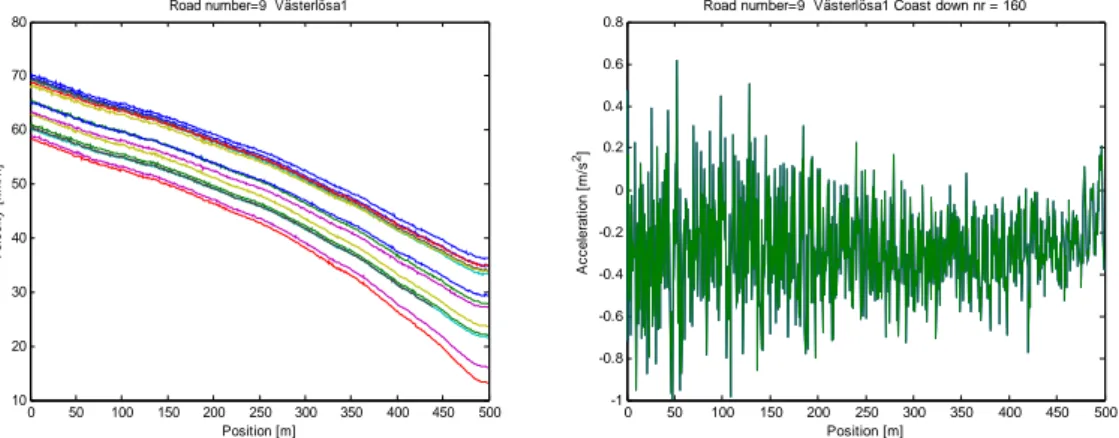
coastdown measurement on this road strip is performed by letting the vehicle roll freely (clutch down, gear in neutral position) between the start and end points. The velocity is measured11 “continuously” along the road strip, see Fig. 3.1. The acceleration is either measured directly or derived from the velocities.

Figure 3.1 Velocity curves for several coastdowns with varying initial velocities along one particular road strip. The curves are almost parallel which indicates that the measurement conditions have been (almost) identical. To the right, the acceleration curve for one specific coastdown. Typically, strong fluctuations occur, caused by small measurement errors.

The various resistive forces acting on the vehicle will make it slow down. RR is one of these forces. The larger the RR, the larger the retardation becomes. By performing several coastdown measurements, under various conditions, it is possible, by using regression analysis, to distinguish and isolate the contributions of the different resistances acting on the vehicle. In particular, if the measurements are performed on different roads with varying road surface properties, it is possible to compute the additional rolling resistance as a function of road surface variables.

3.2 Model

structure

The basis for a mathematical model for coastdown is Newton’s second law. The total force acting on the vehicle is the sum of the gravitational force and the drag force, where the drag force can be assumed to consist of: rolling resistance, air resistance, side forces resistance and transmission resistance (including losses in the bearings).

11_{A possible alternative might be to measure the velocity only at the start and end points. This would} imply a different analysis method than has been used in this report.

0 50 100 150 200 250 300 350 400 450 500 10 20 30 40 50 60 70 80 Position [m] V e lo c ity [k m /h ]

Road number=9 Västerlösa1

0 50 100 150 200 250 300 350 400 450 500 -1 -0.8 -0.6 -0.4 -0.2 0 0.2 0.4 0.6 0.8 Position [m]

Road number=9 Västerlösa1 Coast down nr = 160

A cce le ra ti o n [m /s 2]

(16)

(3.1) The various forces are supposed to depend on the following variables:

Gravitation force: Fgrav = mg sin(θ)

Side force resistance: Fside = Fside(v,m,R, θ, σ)

Transmission resistance: Ftrm = Ftrm(v)

Rolling resistance: FRR = FRR(v, m, T, IRI, MPD)

Air resistance: Fair = Fair(v, A, ρ, w, α)

where

m is the mass of the vehicle Me is the inertial mass

g is the standard value of gravitational acceleration

θ is the longitudinal slope of the road

v is the speed of the vehicle

R is the radius of curvature of the road σ is the crossfall of the road

T is ambient temperature

IRI is the IRI measure of road unevenness

MPD is the mean path depth measure for macrotexture A is the cross sectional area for the vehicle

ρ is the density of air p is the air pressure w is wind speed

α is wind direction (relative to the velocity vector of the vehicle)

Cside, CL, CLbeta, Cr00, CrTmp, CrMPD, CrIRI, CrIRI_V are constant coefficients

In more detail:

Fside=Cside ∙Fy2

Fy=m∙(cos(σ)∙v2/R-g∙sin(σ)∙cos(θ)) (3.2) Fair = (CL+CLbeta∙sin(β)) ∙cos(β) ∙A∙ρ∙vlr2/2 (3.3)

vlr = (v2+ 2∙v∙w∙cos(α) + w2)0.5 β = arccos((v + cos(α)∙w)/vlr) ρ = (348.7/1000)∙(p/(T+273))

For the rolling resistance the following model can be used.

(17)

The transmission resistance can be modeled as a constant term independent of the mass of the vehicle12.

Ftrm = Ctrm (3.4)

Combining the equations in the previous section yields the following general equation:







tmp MPD IRI IRI V



side y air

z trm z e F F C v IRI Cr IRI Cr MPD Cr T Cr Cr F C F dt dv M                    2 _ 00 20 sin (3.5) where Fz = mg.

When applied to measurement data, this equation gives rise to an algebraic, strongly overdetermined, equation system from which the unknown coefficients, Ctrm, Cr00, etc,

can be determined by regression.

3.3 Model

discussion

The suggested model for RR, Eq. 3.5, is far from obvious. For example, the additivity of effect of ambient temperature (T) can be questioned. It might be more appropriate to assume a multiplicative effect of T. Also, the effect of temperature might be more closely related to the terms pertaining to a deformation of the tyre (Cr00 and CrMPD)

rather than to the terms associated with losses in the suspension (CrIRI).

One might also hesitate whether a combined speed-MPD term, CrMPD_V ∙MPD∙(v-20),

should be included into the model. Drum measurement data indicate that such a term should not be included, but no certain conclusions can be drawn from them. Another possibility is to include power terms, e.g., IRI 2.

Similar doubts concerning the transmission model is justified. It is reasonable to believe that losses in the transmission should depend on the speed of rotation of the rotating parts of the transmission.

Some authors suggest13_{that RR is slightly non-linear with respect to the normal force (a}

quadratic function). This effect is ignored in present study.

3.4 Equipment

Coastdown logging:

The GPS equipment VBOX 3i from Racelogic has been used to measure the velocity, see Fig. 3.2 and 3.3. VBOX measures speed and distance with a frequency of 100 Hz. Measurements are based on the Doppler effect, which means that speed (not position!) is the primary quantity being measured. In situations where the signals from satellites are of lower quality (for short time periods), VBOX uses an IMU (Inertial Measurement Unit) to interpolate and improve the speed curve. The IMU houses three yaw rate sensors and three accelerometers. As a power supply, an extra car battery is used. The equipment includes an antenna which is mounted on the top of the vehicle.

12_{It would, however, have been reasonable to model the transmission losses as a function of speed. This} was not done.

(18)

Figure 3.2 The VBOX GPS unit.

Figure 3.3 Equipment for coastdown measurements. On the floor: a car battery and the VBOX inertial measurement unit (IMU) containing accelerometers and yaw rate sensors (blue box). On the couch: the VBOX GPS unit (blue box) and the receiver of the start and end reflex signal (white box).

Device to detect start and end points of a test road:

In order to determine the exact position of the vehicle for any given time, reflexes have been positioned at the road side at the start and end points of the road strip14_{. On the}

right side of the vehicle an optical sensor is mounted, which registers the exact time point when the sensor passes the reflex. The registration is merged together with the VBOX GPS data. This will eliminate any uncertainties concerning the vehicle’s position during the coastdown.

(19)

Weather station:

A weather station measuring wind speed, wind direction, air temperature, air pressure and humidity, was positioned at a suitable location beside the road. Registrations were done once per minute. Wind speed was obtained by averaging the (absolute) wind speed each second (without taking wind direction into account). Wind direction was sampled once each minute. For the HGV, road surface temperatures were measured at stationary stations, which are located rather distant from the road strips (up to 20 km away).

3.5 Test

roads

Eight test roads in the vicinity of Linköping were selected for the coastdown

measurements. The primary selection criterion was to obtain as wide range in MPD and IRI as possible. Also, the road strips should be straight and the slope should not exceed 1%. Moreover, trees or buildings were not allowed to shadow the GPS signal.

In Appendix B, road surface quantities for each test road are described in more detail. The road surface data was measured using a road surface tester (RST) from VTI. Data were collected for each 20 meter segment.

Longitudinal slope was measured with particular precision. For most of the test roads the elevation was measured every 100 meters using high precision GPS equipment and interpolated in between by using the road profile from the RST. Slope was measured along one driving direction and then mirrored onto the opposite driving direction.

3.6 Test

vehicles

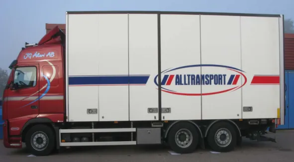
Coastdown measurements were done with two test vehicles, a private car (Volvo 940) and an HGV (without a trailer) normally used for long-distance freight transport, see Fig. 3.4. More detailed vehicle data is given in Appendix A.

For the private car two different types of tyres were investigated: a normal tyre and a studded winter tyre for icy road conditions. One purpose with this setup was to

investigate if there were any significant differences between these tyre types concerning the influence of road surface on RR. Tyre details are shown in Appendix A.

(20)

Figure 3.4 The private car and the heavy vehicle used for coastdown measurements.

3.7 Coastdown

measurements

For each test road, six coastdown measurements were performed in each direction15. Whenever a disturbance of any kind arose (e.g. encountering a large HGV) the driver pushed a special button registering in the output files that the measurement was interrupted. Afterwards, during the analyses, it was easy to remove the disturbed data. When possible, the initial velocity for the coastdowns was varied according to a predetermined scheme16: 90km/h, 50, 75, 90, 50, 75km/h.

The procedure for measuring and adjusting the tyre pressure differed for the private car and the HGV. For the private car, the tyre pressure was checked (and adjusted if

needed) when arriving at a new test road. For practical reasons, the tyre pressure for the HGV was measured (and adjusted) only once a day, in the morning before the

coastdown measurements started.

Before beginning any measurement, the test vehicle was driven warm. Also, the surface temperature of the tyres17 was measured when arriving at a new test road, using a portable IR temperature sensor.

A problem during the measurements was to keep the vehicle in the correct lateral position on the road. This is important since the road surface quantities (in particular MPD) may vary a lot across the road. The wheels of the coasting vehicle should coincide with the tracks where the RST vehicle had measured MPD and IRI. This was achieved (or at least attempted) by giving the drivers instructions to keep a certain distance from the road side. This procedure is not very satisfactory, and one might suspect that it may be an important error source. A related problem is that the width between the tyres may differ among the vehicles (and also among different axles within

15_{Six coastdowns per road strip and direction were done for the private car but only three for the HGV.} 16_{The initial velocities were proportionally adjusted whenever the speed limit did not allow for the} original velocities.

17_{The tyre surface temperatures have, for two reasons, not been used in the analyses. Firstly, the surface} temperature is not a reliable measure of the temperature inside the tyre. (The tyre pressure might then possibly be a more suitable measure.) Secondly, the temperature sensor yielded rather shaky values.

(21)

the same vehicle). This is particularly a problem for the HGV, which is much broader than the private car and the RST. Some part of the HGV tyres will coastdown outside the track where MPD has been measured, causing an extra error.

A further problem was that the HGV measurements were carried out one year after the road data measurements. In particular, the road macrotexture may have changed during this time period. However, since both measurements were done in the autumn, the seasonal variation should be of less importance, only the long term change of the road surface is relevant.

For the private car, coast down measurements were carried out during the autumn 2009 (see Appendix C for more details). Measurements were only done at low wind18

conditions and no precipitation.

For the HGV, coastdown measurements were done during two consecutive days (Sept 30th – Oct 1st, 2010). On the second day, there was a slight rain, so the road surface was humid but without any water pools. Although the wet surface probably had no

significant direct effect on the measurements, it might have affected the temperature of the road surface and of the tyres, and, hence indirectly, also the RR.

3.8 Data

preparation

From the VBOX, coastdown data were obtained with a frequency of 100 Hz. For each coastdown, data was merged to road data, vehicle data and meteorological data. In this process, due consideration of the position of the IR sensor and of the antenna for the VBOX, relative to the center of gravity of the vehicle, was taken. The inclination of the test vehicle was computed from (interpolated) road altitudes of the frontal and rear axle. Meteorological data was computed for the minute interval that contained the vehicle’s passage of the middle point of the road strip. For the private car, air temperature is used, while for the HGV the road surface temperature has been taken.

An observation was declared unacceptable, whenever any of the following condition was satisfied:

 Number of satellites in contact was lower19_{than 8 (or larger}20_{than 14).}

 The driver had pushed the button signifying that the coastdown had been interfered by the surrounding traffic or that the coastdown was interrupted for some other reason (e.g. the vehicle had stopped).

 Wind speed exceeded 1 m/s. (In that case the whole coastdown was discarded.) In the next step data were aggregated to 25 meter intervals (along the road strip). There were essentially two reasons for this: firstly, it is advantageous to reduce the very large amount of data. Secondly, it was found in the ECRPD project that using very short

18_{Sometimes, the wind unexpectedly started to blow during the measurements. In the data analyses,} however, all data for which observed wind speed exceeds 1 m/s has been discarded (for the private car). 19_{VBOX provides an estimate of the number of satellites from which acceptable signals were received.} This estimate gives an indication of the quality of the observation. The maximum number of satellites was usually approx 12. Due to obscuring objects (houses, trees, etc) the number of satellites were often much lower. We decided that a minimum of 8 satellites was required for acceptable precision.

20_{In many cases, reflexes at the start and end points of the road strip could interfere with the ordinary} satellite signals, giving rise to a virtual number of satellites being much larger than 12. These observations were also discarded.

(22)

aggregation intervals yields less precision in the final result. To some extent, taking averages over the data seems to smooth the errors beneficially.

If any of the observations within the aggregation interval had been declared unacceptable, then also the whole aggregated observation (25 m) was declared unacceptable and was discarded. As a consequence a large amount of data was

discarded. (For the private car 44% of the aggregated observations were discarded.) The reason for this precautionary procedure is the idea that a few accidental erroneous observations may be much more damaging than the benefits of a large number of “correct” observations.

The regression models were then applied to the aggregated observations. All computations were done using the statistical package21 R.

(23)

4 Accuracy and reliability issues

4.1 Error sources and their possible influence on the result

Rolling resistance computations from coastdown measurements involve a large number of potential error sources:

 Errors or inexact values in vehicle parameters: weight, moment of inertia of wheels, tyre pressure, tyre temperatures, etc.

 Errors in road surface quantities: Slope, MPD, IRI, etc.

One particular problem may be of special importance: does the coastdown vehicle measure in the same tracks in which road data were measured?

 Errors in meteorological data: wind (level and direction), ambient temperature, air pressure. In particular, the wind measured by the weather station is not necessarily the same as the wind the vehicle is exposed of.

 Errors in GPS data: velocities (the accuracy in these is strongly related to the number of available satellites)

 Incidental errors during measurements: disturbances from other vehicles, etc.  Numerical problems when processing data:

o correlations between explanatory variables (in particular between MPD and IRI or between these and meteorological data). Such correlations may give rise to an ill-conditioned matrix and to decreased accuracy in results

o instabilities when accelerations are computed from velocities o which aggregation level for data is optimal

o imperfect synchronization when merging data from different sources  Defects in model description. Linear or non-linear relationships? Is MPD the

most suitable measure for macrotexture to explain RR?

Most of the error sources listed above have been extensively discussed in [ECRPD, 2009].

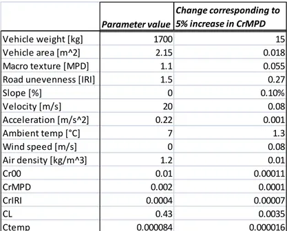
When designing the measurements it is important to identify which of the possible error sources have the biggest influence on the result. Table 4.1 may give some hints on which parameters that are most important in this regard.

(24)

Table 4.1 Illustration of the sensitivity of rolling resistance computations to some input parameters. “Change corresponding to 5% increase in CrMPD” should be interpreted as: “the amount of change needed in the variable to have the same effect on the total resistive force acting on the vehicle as a 5% increase in the coefficient CrMPD would have had”. The numbers have been computed by applying the equations in Sec. 3.2.

The numbers in Table 4.1 illustrate very clearly the challenge that rolling resistance measurements offers. An error of size 0.1% in slope or 0.001 m/s2 gives rise to an error in the force acting on the vehicle that is of the same size as a 5% change in the MPD coefficient, CrMPD, would have had. Thus, a very small (systematic) error in some variables may threaten the accuracy in CrMPD.

Fortunately, the situation is not quite as bad as Table 4.1 might suggest. For example, unbiased random errors will be “cancelled” in the regression. In [ECRPD, 2009] it is shown that the fluctuations in acceleration are often almost harmless, in spite of the fact that these fluctuations may be of the order of 1 m/s2, i.e. a factor 1000 larger than the number given in the table.

On the other hand, systematic errors can be devastating. If, for instance, road macro-texture (MPD) is measured with a systematic error of 0.05, then this will cause an error in CrMPD in the order of 5%. An erroneous value for the vehicle area will also affect results, but only the air coefficient, CL, not CrMPD or any of the other coefficients. Meteorological variables, in particular wind speed, wind direction and temperature, as well as tyre pressure is of special importance since they may vary from one

measurement occasion to another and they do not cancel. We will call these “disturbing variables”.

4.2 Measurement strategies to maximize the accuracy

Quantities affecting vehicle dynamics but not being of primary interest (“disturbing variables”), such as temperature or wind speed, can be handled in either of two ways:

 Compensate for the disturbance by adjusting the right hand side (y) in the regression. Parameter value Change corresponding to 5% increase in CrMPD Vehicle weight [kg] 1700 15 Vehicle area [m^2] 2.15 0.018 Macro texture [MPD] 1.1 0.055 Road unevenness [IRI] 1.5 0.27 Slope [%] 0 0.10% Velocity [m/s] 20 0.08 Acceleration [m/s^2] 0.22 0.001 Ambient temp [°C] 7 1.3 Wind speed [m/s] 0 0.08 Air density [kg/m^3] 1.2 0.01 Cr00 0.01 0.00011 CrMPD 0.002 0.0001 CrIRI 0.0004 0.00007 CL 0.43 0.0035 Ctemp 0.000084 0.000016

(25)

 Include the disturbing variable among the explanatory variables and estimate its coefficient by regression.

Which of these strategies is the most suitable depends on how much the disturbing variable can be expected to vary. If, for instance, temperature can be expected to vary very little, then it is not advisable to estimate it by using regression, since the

uncertainty in the temperature coefficient can then be expected to be large it can easily get a wrong sign and be more harmful22 than beneficial. If we want to determine the influence of temperature by regression, then measurements should be done during more extreme temperature conditions, obtaining a large span in temperatures. On the other hand, measuring at very different temperatures, high correlations between road surface properties and temperature may arise23. This risk might be reduced by performing more than one series of measurements, at random temperature conditions. This will, however, dramatically increase the cost for the measurements.

We believe that the most economical and reliable approach should be to first study each of the disturbing variables (temperature, wind, etc.) separately, making simple (one variable) regressions on data where the particular variable has as extreme values as possible and all other variables are as constant as possible. For instance, the temperature coefficient may be estimated on coastdown data from one specific location (road) at very high and low temperatures but always low wind speed. The regression is done with fixed (preliminary) values for all the other coefficients.

Once this has been done for all the disturbing variables, the computations of the road surface influence (CrMPD and CrIRI) may be done, preferably having as constant temperature as possible and adjusting the y vector for temperature effects.

Another important issue is to avoid correlations between IRI and MPD. High

correlations will give rise to large confidence intervals in the corresponding parameter estimates. This can be avoided by carefully selecting the test roads. Similarly, high correlations between e.g. MPD and other quantities, especially meteorological data, can be harmful for the precision in results.

4.3 Methods for assessing and improving accuracy in regression

There exist a large number of numerical and statistical methods and techniques for assessing and improving accuracy in results from multiple regression. In this section a brief review of such methods is given. Most of them have been applied (or at least considered) on data in this project.

Simple checks to clean data from incidental errors

Initially, it is important to “clean” data from large measurement errors of incidental character (and errors arising in the data processing as well). We have only accepted GPS data based on at least eight satellites (of a maximum of approximately 12

satellites). Also, coastdowns prematurely interrupted or disturbed by surrounding traffic must be removed. In spite of these precautions some incidental errors may still exist. It

22_{Admittedly, the damage should not be very grave since the correction becomes rather small for narrow} temperature intervals.

23_{The different road surfaces have been chosen to possess very different road surface characteristics. If} we are unfortunate, coastdowns on extreme road surfaces may have been done at “extreme” temperatures.

(26)

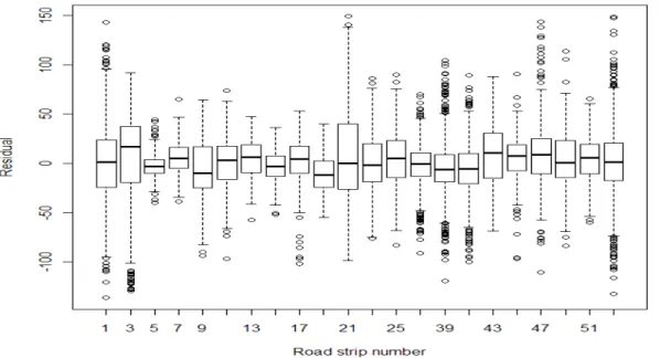
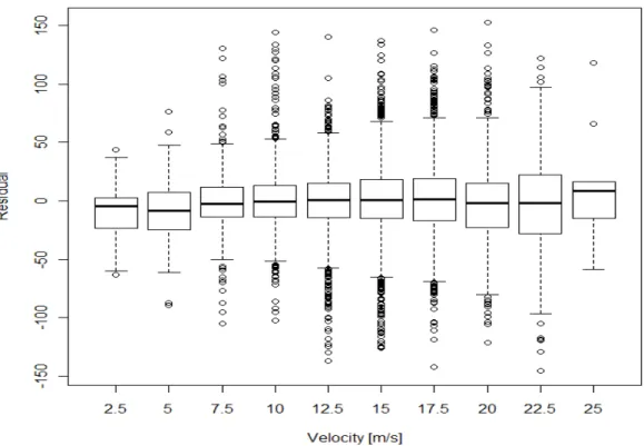
is very useful to plot the velocity curves as a function of position of all the coastdowns performed at one specific road strip and direction. (Data have initially been aggregated to one meter segments.) Even rather small deviations between the curves can be detected by ocular inspection. On more aggregated data (e.g. 25 meters) acceleration can be studied similarly. Finally, when a regression has been performed it is useful also to plot the residual as a function of position (for one specific road strip and direction) or as a function of road strip and direction or as a function of coastdown number. Studying the residuals is very instructive not only to detect any errors in data but also to find out if the applied model is suitable.

Standard statistical diagnostics

When applying a linear regression (model) using any standard statistical package (SPSS, R, SAS, …) various statistical diagnostics describing the quality of the model are presented. For example, for each regression coefficient the standard error, t value, p value and a (95%) confidence interval can be obtained. However, it is important to note that the confidence intervals for the model coefficients are only reliable provided that the error satisfies specific conditions (i.e., that the model is “correct” in some sense). In reality, these conditions may not be satisfied and the confidence intervals can be

misleading.

Perturbation analysis

A very natural question to ask in this context is: “If the measurements (or the

computations) had been carried out in some other way, what would the outcome have been and how much would it have differed from the present results?”. Perturbation analysis systematically addresses this question. In [ECRPD, 2009] a very extensive perturbation analysis was performed for rolling resistance calculations from coastdown measurements. Besides giving an idea of the sensitivity of the results the analysis can also be helpful for identifying errors in data.

The analysis is conceptually very simple but somewhat cumbersome to apply. In order to limit the effort one should focus on a few matters, for instance:

1. How would results have differed if one of the road strips had been skipped? 2. How does the aggregation of data affect result?

3. How do errors in slope measurements affect results? More advanced statistical techniques

 Resampling techniques: This is a family of methods that explores the

information contained in the data material by selecting new data sets from the existing one. Bootstrapping is maybe the most well-known of these methods. The information contained in available data is efficiently exploited and can provide a better estimate of uncertainties if data do not fulfil the standard assumptions on the error that conventional theory is based upon.

 Ridge regression: An important threat to accuracy when applying multiple regression is when there is a strong correlation between two (or more) explanatory variables (multicollinearity). Multicollinearity causes the design matrix to become ill-conditioned and consequently yields larger uncertainties in (some of) the estimated coefficients. Ridge regression is an example of a

(27)

to solve a slightly modified problem in which the multicollinearity is less pronounced and draw conclusions from that.

 Row scaling (weighted least squares): This is a technique for improving accuracy in regression whenever the observations (measurements) have very different precision or reliability. The idea is to give equations (measurements) different weights; a larger weight is put on the more reliable observations. Row scaling might also be used whenever the amount of data is unevenly distributed. (E.g. MPD values in some intervals are much more frequent than in others.)  Total least squares (TLS): In the literature, some authors advocates the use of

total least squares instead of ordinary least squares whenever there are (large) errors in the explanatory variables (“errors-in-variables models”). These errors might contribute to make the assumptions for standard error theory invalid. The TLS method does take into account such errors in a more proper way. TLS is usually not implemented in standard statistical tools (SPSS, SAS, R, S++).  Theoretical error bounds: In the science of numerical analysis much effort has

been devoted to deriving strict error bounds for regression results by assuming that errors in input data is bounded by some value. However, it seems difficult to apply these error bounds in a fruitful way for this type of problems.

4.4 How to choose a model?

Of vital importance when applying the coastdown technique combined with regression is to have a realistic, not too complicated, qualitative model for the dependencies between road surface quantities and RR. At least for the influence of macrotexture, a simple theoretical framework for the description of such dependencies is to our

knowledge not available. On a very detailed level, partial differential equations may be formulated and solved numerically to simulate24 the behavior of the tyre and to calculate energy losses, but what we rather need here is a simplified model in terms of a few basic quantities describing the road surface and meteorological data. A complicating matter is that not only RR has to be taken into account but also other effects, such as air

resistance and transmission losses.

In lack of a theoretical basis we may speculate about the form of the model, guided by our intuition. One can have an idea about which parameters should be included. It is, for example, well-known that temperature is an important factor. From start we have

assumed that MPD and IRI are two road surface quantities that should be included in the model25. However, as discussed in Sec. 3.3, there are many degrees of freedom when forming the model expression and the suggested model, given in Eq. 3.5, is far from obvious.

24_{We believe that, by a systematic study of the result from such simulations, it should be possible to} create a simplified “macro” model which only depends on a few variables and undetermined parameters, which ignores all the details needed in a simulation. The parameters can be determined from coastdown or other measurements.

25_{Determining which road surface measures that are the most appropriate ones to use when describing the} influence of road surface on RR is an important research task. In [ECRPD, 2009] a minor investigation was carried out, comparing various combinations of RMS measures and MPD and IRI. As a (rather crude) criterion for best model the R2_{value was used. No combination of two measures was found} superior to using MPD and IRI.

(28)

To select one viable model, we must be guided by observed data. It is, however, a very difficult and complicated matter to determine which model is the “best” one and to determine if that one is a reasonably correct picture of reality. First of all, data is subject to various correlations and measurement errors which might be both systematic and random. Secondly, we may be guided by different criteria. The standard statistical indicators (R2 value, t value for coefficients, etc.) presuppose that the model is “correct” in the first place. An alternative guidance is the “stability” of a model. If data is

reasonably reliable a necessary requirement of a model is that it should be stable, i.e. the parameter estimates should not change much when removing or changing some data. A natural way to study the stability is to systematically remove all data from one road strip, one road strip at a time. This procedure answers the question: what result would we have obtained if we had skipped measurements on one of the road strips?

Unfortunately, stability is not sufficient to determine a valid model it can only be used for rejecting inappropriate ones.

(29)

5 Analyses

and

results

In this section results from analyses of coastdown measurements are presented. Also, comparisons are done with results from trailer and laboratory drum measurements.

5.1 Results for a private car

5.1.1 Data

Analyses have been done using several datasets obtained from coastdown measurements:

Sd1: First series of coastdown measurements using normal tyres Sd2: Second series of coastdown measurements using normal tyres Dd1: First series of coastdown measurements using studded winter tyres Dd2: Second series of coastdown measurements using studded winter tyres

W: Four series of coastdown measurements with different weights using the normal tyres

ECRPD1: First series of coastdown measurements using the normal tyres ECRPD2: Second series of coastdown measurements using the normal tyres

The first four datasets have been collected in connection with this project. The last two originates from the ECRPD project.

Each of the coastdown26 series Sd1, Sd2, Dd1 and Dd2 contains data from 8 different road strips27_{. Coastdowns have been done essentially in the same way as in the ECRPD}

project (but using different equipment): six coastdowns in each direction of a road strip with varying start velocities.

The four series in W have been measured on the same road strip but with different loads. Everything else has been kept as constant as possible. W has only been used in Sec. 5.1.3.

Each of the series ECRPD1 and ECRPD2 were performed on 14 different road strips. For more details on ECRPD data, see [ECRPD, 2009].

All computations have been done with aggregations of data to 25 meters (if not otherwise mentioned). Measurements for which wind speed exceeds 1 m/s have been excluded.

5.1.2 Choosing an appropriate model

Introduction

In order to illustrate the difficulties that arise when selecting an appropriate model for the driving resistance, we present in this section some results for a number of different model suggestions. Also, the results here give some indications how stable results are for different model choices. Computations have been done on the data set

26_{More details of measurement data is found in the appendices. Parameters for the test vehicles, including} tyres, are described in Appendix A. Test roads are described in Appendix B and the coastdowns in Appendix C and D.

(30)

Sd1+Sd2+Dd1+Dd2+ECRPD1+ECRPD2, described in the previous section. All results in this section refer to an air temperature being 5 ⁰C. Transmission resistance has been compensated for by reducing the total resistance by a fix quantity, 65.5 N. This value is derived from measurements in Sec. 5.1.3.

Note that the models here include besides pure RR also resistance due to side forces as well as air resistance.

The models studied consist of the following ingredients28:

Cr00 * Fz: basic rolling resistance, Fz is the normal force

CrMPD * MPD * Fz linear effect of MPD

CrIRI * IRI * Fz linear effect of IRI

CrIRI_V * IRI *( v-20) combined effect of IRI and speed

CrIRI2 * IRI^2 quadratic effect of IRI

CrSide * Fy^2 the side force effect (see Eq. 3.2)

CrTemp*(5-T)*Fz temp effect relative to 5 ⁰C, T is ambient temp

CL * AIR air resistance (see Eq. 3.3)

CLbeta * AIR*sin(beta) correction29 term for air resistance where AIR = A*VLR^2/2*DNSL*cos(beta) Moreover, three sets of dummy variables30 are introduced, one set for the six

measurement series (c1, c2, ..., c6) another set for the 23 road strips31 (s1, s2, ..., s22) and a third set for the lane-directions32_{of each road strip (r1, ..., r22). Each of the}

coefficients, ci, can be interpreted as the effect that the i:th measurement series has on the total resistance. E.g., the first measurement series can be concluded to have a resistance differing by c1 units from the average of all measurement series, provided all else equal. Likewise, the road strip dummy, si, were introduced to detect the effect that the i:th road strip has on the total resistance. Similarly, the lane-direction dummies were introduced to detect if the lane-direction has any effect on the result. The dummy

variables are powerful tools to detect systematic differences between different categories or classes that cannot otherwise be explained by the model.

28_{All quantities starting with a ”C” denote parameters whose value is to be determined by regression.} 29_{The reason for introducing a correction term is that a constant value for CL does not properly account} for side wind effects.

30_{The dummy variables for the measurement series (c1, c2, …, c6) are called “effect dummies”, see} [Kutner et al, 2004]. Each of the dummies may assume one of the values 1,0,-1. For example: ci=1 for the

i:th measurement series and ci=0 for all other series except the last one (c6), where ci=-1. Only c1,…,c5

are introduced in the model. The coefficient for the last dummy may be retrieved by the condition that the sum of all coefficients must be equal to 0.

31_{The dummy variables for the roads are also “effect dummies”. They are constructed in the same way as} the measurement series dummies.

32_{The dummies for the lane direction, ri, are not effect dummies but a homemade combination of road} specific dummies (si) and directional dummies. The lane-directional dummies are defined by

ri=((d==1)-d==2))*si, for each road strip i. d denotes the direction of a lane (d=1 means forward direction, d=2

(31)

Models without dummies:

1a. y = Cr00*Fz + CL*AIR

2a. y = Cr00*Fz +CrTemp*(5-T)*Fz + CrSide*Fy^2 + CL*AIR

3a. y = Cr00*Fz + CrTemp*(5-T)*Fz + CrMPD*MPD*Fz + CrSide*Fy^2 + CL*AIR

4a. y = Cr00*Fz + CrTemp*(5-T)*Fz + CrMPD*MPD*Fz + CrIRI*IRI*Fz + CrSide*Fy^2+CL*AIR 5a. y = Cr00*Fz + CrTemp*(5-T)*Fz + CrMPD*MPD*Fz + CrIRI*IRI*Fz + CrIRI_V*IRI*(v-20)*Fz

+ CrSide*Fy^2 + CL*AIR

6a. y = Cr00*Fz + CrTemp*(5-T) *Fz + CrMPD*MPD*Fz + CrIRI*IRI*Fz + CrIRIV*IRI*(v-20)*Fz

+ CrSide*Fy^2 + CL*AIR + CLbeta*AIR*sin(beta)

The same models as above with dummies33 for measurement series:

1b. y = Cr00*Fz + CL*AIR + c1 + c2 + c3 + c4 + c5

etc.

The same models as above with dummies for measurement series and for lane direction:

1c. y = Cr00*Fz + CL*AIR + c1 + c2 + c3 + c4 + c5 + r1 + r2 + r3 + … + r22

etc.

Attempts have been made to use also the road specific dummies (s1+s2+…+s22). They resulted, however, in unstable and seemingly unreasonable values and are therefore excluded here.

Comparisons between models

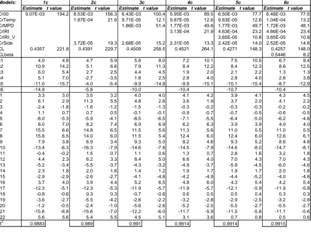
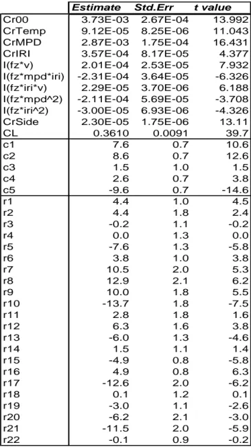
In Tables 5.1a, b and c, results are shown when estimating the models 1a, …,6c on the entire dataset. In general, very large t-values are obtained for most parameters,

indicating relatively low random errors in the estimates. Switching from one model to another may, however, result in rather large changes in the parameter values. Some of these variations are natural. For instance, the coefficient Cr00 should differ between models 2a, 3a and 4a, since in model 2a the term Cr00 will comprise also much of the MPD and IRI effects.

However, some quantities that might be expected to be constant also vary significantly. For example, CrTemp, differs very much between model 2b and 3b, and also in general between the models with and without dummy variables. It is expected from literature that the values around 1e-4 is the more reasonable for CrTemp.

Another coefficient that should not vary is CrSide. [Nordmark, 1985] has estimated

CrSide to be 2.35e-5 for a private car. This value agrees very well with results for

models 6a, 6b, 4c and 5c. CrSide is a useful validation coefficient for the models. It should however be noted that only the crossfall has been taken into account when computing the side forces acting on the vehicle, while the road curvature has been neglected (most of the road strips are almost straight), see Eq. 3.2.

33_{For notational simplicity we skip the coefficients for the dummy variables. Strictly, model 1b should} have been written y=Cr00*Fz+CL*AIR+C1*c1+C2*c2+…

(32)

Table 5.1a. Estimated model parameters for various models without any dummy variables.

Table 5.1b. Estimated model parameters for various models with dummy variables for the measurement series.

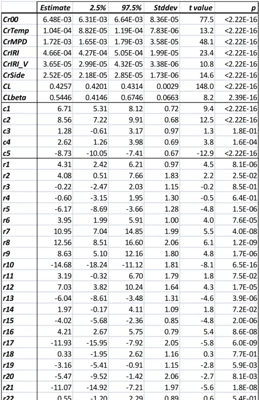
Table 5.1c. Estimated model parameters for various models with dummy variables for the measurement series and for the road directions.

Models:

Estimate t value Estimate t value Estimate t value Estimate t value Estimate t value Estimate t value Cr00 8.82E-03 187.5 8.33E-03 158.0 6.33E-03 98.5 5.88E-03 88.4 6.47E-03 76.0 6.43E-03 76.0 CrTemp 2.25E-04 33.6 1.90E-04 30.5 1.96E-04 32.1 1.98E-04 32.6 1.99E-04 32.9

CrMPD 1.72E-03 47.3 1.63E-03 45.2 1.63E-03 45.2 1.58E-03 44.1

CrIRI 3.09E-04 21.2 4.53E-04 23.1 4.56E-04 23.4

CrIRI_V 3.62E-05 10.9 3.62E-05 11.0

CrSide 4.03E-05 21.5 3.54E-05 20.6 3.18E-05 18.7 3.26E-05 19.3 3.31E-05 19.7 CL 0.4364 220.5 0.4436 238.3 0.4526 263.2 0.4533 268.4 0.4271 146.2 0.4254 146.2 CLbeta 0.7772 11.8 R2 0.9868 0.9885 0.9903 0.9906 0.9907 0.9908 5a 6a 1a 2a 3a 4a Models:

Estimate t value Estimate t value Estimate t value Estimate t value Estimate t value Estimate t value Cr00 8.98E-03 195.2 8.47E-03 157.5 6.37E-03 100.1 5.88E-03 89.0 6.50E-03 77.5 6.48E-03 77.4 CrTemp 1.84E-04 21.0 9.49E-05 11.7 9.72E-05 12.2 9.82E-05 12.4 1.04E-04 13.1

CrMPD 1.87E-03 51.1 1.78E-03 49.4 1.77E-03 49.5 1.73E-03 48.0

CrIRI 3.28E-04 22.8 4.83E-04 25.0 4.85E-04 25.2

CrIRI_V 3.87E-05 12.0 3.87E-05 12.0

CrSide 3.56E-05 18.6 2.63E-05 15.1 2.21E-05 12.9 2.29E-05 13.4 2.37E-05 13.9 CL 0.4409 232.2 0.4439 240.0 0.4545 269.2 0.4553 275.4 0.4273 149.7 0.4259 149.4 CLbeta 0.5617 8.4 c1 3.828 4.6 4.5 5.6 5.6 7.6 7.2 9.9 7.5 10.3 6.7 9.2 c2 10.83 13.9 5.2 6.6 7.9 11.0 8.4 12.0 8.4 12.1 8.6 12.3 c3 6.71 6.0 3.4 3.1 5.2 5.2 2.4 2.4 2.3 2.4 1.5 1.5 c4 5.223 7.1 -2.5 -3.1 1.9 2.7 3.0 4.2 2.9 4.1 2.7 3.9 c5 -11.41 -16.1 -4.5 -6.1 -10.4 -15.2 -10.3 -15.5 -10.3 -15.5 -8.9 -13.1 c6 -15.181 -6.189 -10.314 -10.626 -10.851 -10.552 R2 _0.9879 _0.9886 _0.9907 _0.9911 _0.9912 _0.9912 5b 6b 1b 2b 3b 4b Models:

Estimate t value Estimate t value Estimate t value Estimate t value Estimate t value Estimate t value

Cr00 9.07E-03 194.2 8.53E-03 156.3 6.43E-03 100.4 5.95E-03 89.5 6.50E-03 77.7 6.48E-03 77.5

CrTemp 1.87E-04 21.6 9.71E-05 12.1 9.87E-05 12.6 9.83E-05 12.6 1.04E-04 13.2

CrMPD 1.86E-03 51.4 1.77E-03 49.6 1.77E-03 49.7 1.72E-03 48.1

CrIRI 3.13E-04 21.9 4.63E-04 23.2 4.66E-04 23.4

CrIRI_V 3.65E-05 10.8 3.65E-05 10.8

CrSide 3.72E-05 19.3 2.68E-05 15.2 2.31E-05 13.3 2.42E-05 14.0 2.52E-05 14.6

CL 0.4357 221.8 0.4391 229.7 0.4509 258.5 0.4521 264.1 0.4271 148.3 0.4257 148.0 CLbeta 0.5446 8.2 c1 4.0 4.8 4.7 5.9 5.8 8.0 7.2 10.1 7.5 10.5 6.7 9.4 c2 10.9 14.2 5.1 6.6 7.9 11.3 8.4 12.2 8.4 12.3 8.6 12.5 c3 6.0 5.4 2.7 2.5 4.4 4.5 1.9 2.0 2.1 2.2 1.3 1.3 c4 5.1 7.0 -2.7 -3.5 1.8 2.5 2.8 4.0 2.8 4.0 2.6 3.8 c5 -11.0 -15.7 -4.0 -5.4 -9.9 -14.8 -9.9 -15.1 -10.1 -15.4 -8.7 -12.9 c6 -14.9 -5.8 -10.0 -10.4 -10.7 -10.4 r1 3.3 3.0 3.5 3.2 4.0 4.0 4.1 4.2 3.9 4.1 4.3 4.5 r2 6.1 2.9 11.3 5.5 4.8 2.6 3.6 1.9 3.7 2.0 4.1 2.2 r3 -2.4 -1.8 -1.6 -1.2 -1.5 -1.3 -0.3 -0.2 -0.3 -0.3 -0.2 -0.2 r4 1.1 0.7 0.7 0.5 -0.1 -0.1 -0.9 -0.7 -0.7 -0.5 -0.6 -0.5 r5 -8.0 -5.3 -5.9 -4.1 -8.5 -6.5 -7.1 -5.5 -6.4 -5.0 -6.2 -4.8 r6 8.0 7.0 8.2 7.4 6.9 6.9 6.2 6.3 3.9 3.9 4.0 4.0 r7 15.5 6.6 14.8 6.5 11.5 5.6 11.3 5.6 11.0 5.5 11.0 5.5 r8 15.8 6.5 14.0 6.0 11.5 5.4 12.4 6.0 12.4 6.0 12.6 6.1 r9 7.9 3.8 6.9 3.4 9.3 5.0 8.2 4.6 9.3 5.2 8.6 4.8 r10 -13.4 -6.3 -16.3 -7.9 -14.6 -7.8 -14.5 -7.9 -14.6 -8.0 -14.7 -8.1 r11 -0.4 -0.2 1.5 0.7 1.1 0.6 1.3 0.7 2.8 1.6 3.2 1.8 r12 4.4 2.3 6.2 3.3 8.4 5.0 6.6 4.0 7.0 4.3 7.0 4.3 r13 -5.2 -3.4 -5.5 -3.7 -4.3 -3.2 -4.9 -3.7 -5.9 -4.5 -6.0 -4.6 r14 2.3 1.8 2.0 1.6 1.4 1.2 1.9 1.7 1.9 1.7 2.0 1.8 r15 -2.9 -2.9 -2.6 -2.7 -4.1 -4.8 -4.2 -4.9 -4.4 -5.2 -4.0 -4.8 r16 3.7 4.0 3.9 4.4 5.2 6.5 4.8 6.0 4.3 5.4 4.2 5.4 r17 -12.3 -5.1 -12.3 -5.3 -11.9 -5.7 -11.9 -5.7 -12.1 -5.9 -11.9 -5.8 r18 -0.8 -0.6 0.3 0.3 -0.7 -0.6 0.6 0.5 0.5 0.4 0.3 0.3 r19 -3.6 -2.7 -5.5 -4.2 -2.6 -2.2 -3.2 -2.8 -2.9 -2.5 -3.2 -2.8 r20 -1.2 -0.5 -2.4 -1.0 -5.6 -2.6 -5.2 -2.5 -5.5 -2.7 -5.5 -2.7 r21 -15.6 -6.8 -15.6 -7.0 -12.2 -6.0 -11.7 -5.9 -11.5 -5.8 -11.1 -5.6 r22 5.6 5.6 5.4 5.5 4.5 5.1 3.1 3.6 0.7 0.8 0.5 0.6 R2 _0.9883 _0.989 _0.991 _0.9914 _0.9914 _0.9915 5c 6c 1c 2c 3c 4c

(33)

The air resistance coefficient, CL, should also be constant provided that the air

correction term, CLbeta, is included. CL differs very little between models 6a, 6b and 6c. In contrast, CL changes significantly when removing the combined term IRI*(v-20). (This might possibly indicate that velocity is not properly described by the models.) An estimate of CL for the probe vehicle is given from manufacturer: 0.37. However, this nominal value may have been affected by measurement equipment and other

modifications.

The R2 value increases slowly when introducing more terms in the model but does not vary dramatically. The introduction of dummy variables slightly increases R2.

The dummy coefficients c1,…,c6 correspond to the measurement series Dd1, Dd2, Sd1, Sd2, ECRPD1 and ECRPD2. The dummy coefficients indicate a systematic difference among the measurement series. These differences cannot be explained by the basic models. Since c1 and c2 is larger than c3,…, c6 it can be concluded that the resistance for Dd1 and Dd2 (studded winter tyres) seems to be somewhat larger than for the ordinary tyres. More surprisingly, the resistance for Sd1 and Sd2 seems to be (much) larger than for ECRPD1 and ECRPD2, in spite of the fact that the same tyres have been used. The nature of this latter difference has not been clarified.

The lane-directional dummies, r1 … r22, are also rather stable. Their values indicate that they may be related to measurement errors in longitudinal slope of the roads. Using lane directional dummies should (at least partly) compensate for errors in longitudinal slope. Comparison between Table 5.1 b and c reveals the effect of these dummies and hence, indirectly, should also indicate the effect of errors in slope measurements.

CrMPD differs very little while CrIRI seems more sensitive.

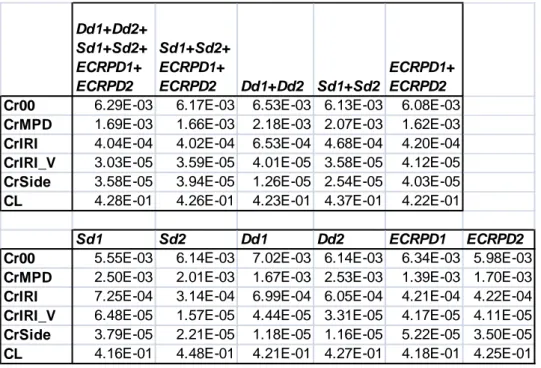
Stability of parameters with respect to subsets of data

By selecting various subsets of data the stability of model parameters can be studied. In Table 5.2, parameter estimates are shown for various datasets for model 5a. Since the variation in temperature is small for some measurement series, yielding unreliable results, we choose to freeze the temperature coefficient to a fix value, CrTemp=1e-4, which is used for adjusting for differing temperatures.

The most stable coefficient is the air resistance coefficient, CL. For single measurement series, the MPD coefficient, CrMPD, varies for ordinary tyres from 1.39e-3 (ECRPD1) up to 2.5e-3 (Sd1). For winter tyres, CrMPD varies from 1.67e-3 (Dd1) to 2.53e-3 (Dd2). For aggregations of measurement series, results become more stable.