This is an author produced version of a paper published in Transportation
Research Part D: Transport and Environment. This paper has been
peer-reviewed but does not include the final publisher proof-corrections or
journal pagination.
Citation for the published paper:
Jevinger, Åse; Persson, Jan A.. (2016). Consignment-level allocations of
carbon emissions in road freight transport. Transportation Research Part D:
Transport and Environment, vol. 48, p. null
URL: https://doi.org/10.1016/j.trd.2016.08.001
Publisher: Elsevier
This document has been downloaded from MUEP (https://muep.mah.se) /
DIVA (https://mau.diva-portal.org).
Consignment-level allocations of carbon emissions in
road freight transport
Abstract
This paper presents and evaluates a new method for how emissions from freight transport routes with single or several points of loading and unloading, can be allocated to individual consignments. The method, called Dedicated Distance Proportional Allocation (DDPA), has been developed based on a literature review, discussions with logistics providers, and analysis. DDPA is designed to have low data processing requirements and be easy to explain to actors involved. Furthermore, it supports several levels of information availability, and accounts for any set of vehicle-limiting factors, as well as prepositioning/repositioning. DDPA has been evaluated in simulations with different levels of information availability, together with three existent allocation methods: the Equal profit method (EPM), the CEN EN16258:2011 standard and the Greenhouse gas (GHG) protocol. The simulations show that the GHG protocol under-allocates the total amount of emissions, on average. EPM and DDPA achieve equal relative savings, whereas for CEN EN16258:2011 and the GHG protocol, relative savings vary, on average. When DDPA is used with low level of information availability, an error is introduced which can be reduced by applying compensation factors. Since DDPA accepts low information availability, the Intelligent Products concept can be applied for computing and storing emissions allocations, at the time of unloading. The results from this study can be used for further development and implementation of consignment allocation methods. Furthermore, by combining DDPA with other environmental load approaches for other parts of a product’s life cycle, a complete life cycle assessment of the product’s environmental impact can be obtained.
1. Introduction
The temperature on the surface of earth continuously rises and the last three decades have been warmer than any preceding decade since year 1850 (IPCC, 2014). The effects of anthropogenic greenhouse gas emissions, together with other anthropogenic drivers, have been shown, with extreme likelihood, to be the dominant cause of the warming observed since the mid-20th century. Different legislation has therefore been imposed by the national governments on companies. In addition to legislation, economic and public image concerns also motivate companies to reduce their transport emissions (Pålsson and Kovács, 2014). For instance, improving environmental performance can be a lever for companies to improve financial results, particularly in regions where carbon tax or emission trading are applied (De Giovanni and Vinzi, 2014; Elhedhli and Merrick, 2012). Piecyk and McKinnon (2010) have investigated to what extent companies with freight transport operations expect climate change to affect their logistics systems in the future. They found that climate change is expected to wield a significant influence on freight transport operations in more than 80% of businesses by 2020. This result highlights the need for companies to understand how to measure and manage road transport emissions (Piecyk and McKinnon, 2010). Piecyk and McKinnon also found that companies are expected to become more heavily involved in various collaboration initiatives in the future to improve the utilisation of their fleets. If companies are to measure their road transport emissions, the emissions from such collaborations must be allocated between the actors involved. As a result, common standards for estimating the carbon footprint of each freight journey are needed (EU, 2011). In addition, breaking down transport emissions to the consignments being transported enables transport actors to make more informed decisions. For instance, inefficient transport with low filling rates can be identified and appropriate actions can thereby be taken to prevent them.
Another reason for calculating product-level carbon footprints have to do with environmental practices and the preferred mode of transport. A shift from road to other modes of transport is commonly suggested as a promising way to reduce emissions from transport operations. A multimodal strategy may also in some cases reduce transportation costs (Rosič, H. et al., 2009). Research shows that one of the reasons this modal shift has not yet occurred (despite considerable political efforts), is inertia in the demand for environmental solutions (Eng-Larsson and Kohn, 2012). Moreover, research also shows that the transport actors have not implemented environmental practices within each mode of transport, to the extent expected (Pålsson and Kovács, 2014). The consumers’ environmental demand is an important driver for environmental practices, since it influences the selection of mode of transport and the carrier (Björklund, 2011; Pålsson and Kovács, 2014), and an increased environmental demand promotes an increased use of environmental solutions. A properly declared product-level carbon footprint has the potential to encourage consumer demand for low-emission products (Kimura et al., 2010) and increase the focus on environmental impacts of different transport solutions. This may,
in turn promote a shift to more environmental transport modes. It might also encourage greater efforts for a reduction of emissions caused by transport; for instance, it may increase the incentive to select low-carbon fuels.
The subject of how to estimate emissions by vehicles, in road freight transport, is well covered by international reports and standards (Boulter and McCrae, 2007; CEN, 2012; DEFRA, 2010; EEA, 2009; GHGP, 2011; NTM, 2010). Information about how to allocate the estimated emissions to the consignments being transported is, however, rather more sparse and the methods presented often show weaknesses (Davydenko et al., 2014). In particular, they are usually primarily designed for transport routes with only a few stops (BSI, 2011; DEFRA, 2010; GHGP, 2011; NTM, 2010). Allocating emissions from transport of one consignment from one point to another, i.e. dedicated transport, is rather straightforward since all emissions, including emissions from any return transport, can be allocated to the consignment in question. Allocating emissions from transport of several consignments from one point to another, is usually also relatively straightforward since all emissions can be allocated to the consignments in question based on, for instance, share of weight or volume (BSI, 2011; NTM, 2010). However, allocating emissions from transport of several consignments, each with different points of loading and unloading in a transport route, adds an extra level of complexity which is only addressed by a few of the allocation methods presented in literature. We believe there is room for improvement of the way such allocations are performed.
The main objective of this paper is to present and evaluate a new method, called Dedicated Distance Proportional Allocation (DDPA), for how to allocate emissions in road freight transport routes with several points of loading and unloading. A secondary objective of this paper is to evaluate three of the allocation methods presented in literature, and compare them with DDPA. The allocation methods selected, denoted as reference methods, are based on: the Equal profit method (EPM), CEN EN16258:2011 and the Greenhouse gas (GHG) protocol (Frisk et al., 2010; CEN, 2012; GHGP, 2011). For the purpose of evaluation, we have designed and developed a new simulation program, which simulates both DDPA and the reference allocation methods in transport routes with different points of loading and unloading of the consignments being transported. The evaluation reveals the strengths and weaknesses of all the methods; in particular in terms of over- or under-estimations. A third objective of this paper is to show how DDPA can be used with different levels of information availability. The information availability levels reflect different transport scenarios, ranging from having reliable information of all types of information required by the methods, to having information that is allowed to change during transport in terms of upcoming stops as well as consignments involved. In particular, this is important when allocation is done at the time of unloading, in more dynamic transport planning scenarios (and not after the transport has ended, when all information is known).
The paper is structured as follows. Section 2 presents a review of existing allocation methods and a motivation of the research. In section 3, the selected reference allocation methods are compared with DDPA, in terms of qualities and characteristics. The information required by the different allocation methods is investigated in section 4. Section 5 gives a detailed description of DDPA. Sections 6, 7 and 8 describe the simulation set-up and report the results of simulations without compensation factors and with them. The paper ends, in section 9, with the conclusions and a discussion of the implications related to this work.
2. Background and research motivation
Much of the ongoing research in emission allocations is dedicated to the emissions caused by a product during its entire life cycle, from cradle to grave (Browne et al., 2005; Schmidt, 2009; Scipioni et al., 2012). The supply chain part of the product life cycle has received particular attention. For instance, several organisations strongly promote product-level carbon auditing of the supply chain (McKinnon, 2010a), and some of the advantages, as well as the problems, associated with product-level carbon auditing have been investigated (McKinnon, 2010a). The need for a commonly agreed standard has been emphasised (Jensen, 2012; Liimatainen and Nykänen, 2011), and though initiatives have been taken for standardisation, differences exist between the standards. In addition to the standards a number of different types of guidelines for how to estimate and allocate emissions also exist; however, there is currently no globally accepted allocation method (Jensen, 2012; McKinnon and Piecyk, 2010; Kellner and Otto, 2012; COFRET, 2011).
A summary of existing emission allocation methods related to road freight transport is presented by Kellner and Otto (2012). They propose to differentiate between methods respecting distances, methods based on other allocation factors than distance, and game theory approaches. The distance-independent methods do not take any transport distances into account. Instead, they allocate emissions, for instance, equally between the consignments being transported, or based on share of weight (or mass, payload etc.) of the consignments. Most of the established carbon auditing standards and specifications belong to the distance-independent category (e.g., GHGP, 2011; BSI, 2011; DEFRA, 2010; NTM, 2010). The distance-dependent methods take different transport distances into account. The amount of emissions allocated to each consignment may hereby depend on, for instance, the distance between the consignment’s point of loading/unloading and the route starting point, or the sum of distances between the consignment’s point of loading/unloading and all other stops along the route (in relation to the corresponding distances of the other consignments). The CEN EN16258:2011 standard belongs to the distance-dependent category. Finally, game theory approaches are based on solution concepts from co-operative game theory, e.g., the Shapley value or the nucleolus (Schmeidler, 1969; Shapley, 1953), can also be used to solve the allocation problem. Game theory-based cost allocation methods used in transports are generally concerned with how transport costs should be allocated to the individual items collaborating in the transport (Engevall et al., 1998; Frisk et al., 2010). These methods usually apply a centralistic approach, assuming that all relevant information about the entire transport is available, and they often have relatively high data processing requirements, involving a larger set of input data, in comparison to other allocation methods found in literature (Frisk et al., 2010; Shapley, 1953; Tijs and Driessen, 1986;
Kellner and Otto, 2012). Furthermore, many of the methods are considered relatively difficult to implement or to understand, since they may involve permutations, linear programming or joint cost assumptions (Kellner and Otto, 2012). The simplest cost allocation method presented by Kellner and Otto, called “Savings cost proportional allocation”, is, however, relatively straightforward. It allocates emissions based on the cost (emissions) that would be incurred if a consignment were transported separately, i.e. the stand-alone cost1, in relation to the stand-alone costs of the other
consignments.
In practice, companies and their customers commonly use software tools to calculate carbon footprints on, for instance supply chain, company- or product-level (McKinnon, 2010b). One of the problems with calculating carbon footprint on product-level is that it is more complicated than, for instance company-level calculation, since it usually involves several actors (Piecyk, 2010). Therefore, some companies restrict their carbon footprint reports to company-level only (Colicchia, 2013). The carbon calculators used for product-level calculations, usually apply one of the allocation methods described by Kellner and Otto (2012). However, these calculators are often criticised for methodological problems (Kellner and Otto, 2012). One problem, which is confirmed by our discussions with logistics providers, is that they are usually based on generalised and aggregated information. For instance, one of the large logistics companies operating in Sweden stated that they allocate emissions to a consignment based on the consignment weight in relation to how much is allowed to be loaded onto the truck, times some pre-defined correction factor (i.e. without using any information on other co-loaded consignments). Furthermore, they only calculate and allocate emissions from one point to another, i.e. without taking the effects of routes with several stops, into account. The use of this methodology is confirmed by another large logistics company in Sweden, who states that they likewise base their emission allocations on consignment weight, without regard to co-loaded consignments.
One of the problems with using the allocation methods found in literature is that they seem to be primarily designed for transport routes with only two or a few stops (BSI, 2011; DEFRA, 2010; GHGP, 2011; NTM, 2010). This means that when they are used for more extensive routes, some of their effects may be considered unfair. For instance, emissions caused by empty transport to a point of loading (prepositioning (CEN, 2012)) and emissions caused by empty transport from the last point of unloading back to a repositioning point, e.g., a home terminal (repositioning (CEN, 2012)) are often not specifically addressed (NTM, 2010; DEFRA, 2010). As a consequence, emission from these transports might be neglected or allocated to only one of the consignments involved in the entire route. Furthermore, emissions are usually allocated without respect to the loading and unloading points of a consignment, in relation to the loading and unloading points of the other consignments involved, or in relation to the route starting/ending points (BSI, 2011; GHGP, 2011; NTM, 2010; DEFRA, 2010; CEN, 2012). This means, for instance, that if a consignment’s loading and unloading points are located far from a home terminal, and the rest of the consignments’ loading and unloading points are located close to the home terminal, the latter consignments will be negatively affected by the former consignment since many allocation methods will allocate a disproportionally high level of emissions to these consignments. Another problem that may cause undesired effects when using existent methods, is that the estimated emissions from source to delivery often are used in combination with only either consignment weight or consignment volume to calculate the emission share (BSI, 2011; NTM, 2010). Since there might be several physical factors limiting the amount of possible load, i.e. limiting factors (DEFRA, 2010), a combination of many limiting factors could be more suitable. Moreover, the limiting factor problem is further complicated by the fact that load weight causes additional transport emissions whereas load volume does not; it only limits the additional volume that can be loaded onto the vehicle. It may therefore not be obvious which factor to base allocations on. Yet another problem with using the existent allocation methods is that they do not support different levels of information availability, which means that many of the methods cannot be used in situations when only little information is available.
Some of the problems above could be solved using a game theory approach instead. However, these methods generally assume all relevant information about the entire transport is available, which might not always be the case, and they often have relatively high data processing requirements, or are considered as difficult to understand. A method which is difficult to understand may be hard to explain to the transport actors involved, which in turn may reduce acceptance.
In summary, we have failed to find consignment-level allocation methods which are designed for transport routes with several points of loading and unloading (including taking the distances between the loading and unloading points, and to the route starting/ending points into account), and which support any set of limiting factors, have low data processing requirements as well as are easy to explain to the actors involved. The objective of this paper is therefore to present a new emission allocation method, DDPA, that:
• account for several points of loading and unloading • account for several (any set of) limiting factors • account for both prepositioning and repositioning
• support different levels of information availability (enabling both centralised and distributed approaches) • are computationally efficient
• are simple in terms of being easy to implement, as well as easy for the actors involved to understand
DDPA has been developed by combining some existing emission allocation methods, with traditional cost allocation methods. It is a distance-dependent method that allocates emissions to a consignment based on the distance the consignment would have travelled if it was transported alone in a separate, dedicated transport (including route
starting/ending points and points of loading/unloading) i.e. the dedicated transport distance. The share of allocated emissions reflects this distance in relation to the sum of the corresponding distances of the other co-loaded consignments. Additionally, the allocation is affected by the limiting factors (e.g. the weight or volume of the consignment in relation to the other consignments), as stated above. By using the dedicated transport distance, emissions caused by distant points of loading or unloading (in relation to other stops) will affect the individual consignments responsible for these stops more, than the other consignments in the route. It also means that the allocations are influenced by the stand-alone cost in relation to the stand-alone costs of the other consignments, as in one of the game-theory approaches described above. In order to support different levels of information availability, DDPA uses estimations in situations when information is allowed to change during transport in terms of upcoming stops as well as consignments involved.
We believe that DDPA has the potential to increase the level of fairness in consignment emission allocations, in the sense that the problems identified above can be reduced. The concept of fairness is relatively subjective in this context. For instance, the solution for what proportion of the total amount of emissions a heavy consignment should receive, in relation to a large consignment consuming most of the space in the transport vehicle, is not obvious. However, we believe that a minimum criteria for a fair emission allocation is that the consignments involved in a transport route should not receive more emissions than if they were transported in separate, dedicated transports. Therefore, DDPA is focused on minimizing the risk of allocating more emissions than this, in addition to reducing the problems with the existent allocation methods (which typically can be considered as unfair, from the aspects described above).
3. Selected reference allocation methods
In order to find appropriate reference allocation methods for the purpose of comparing and evaluating DDPA, we have performed a comprehensive literature review. The review resulted in three different reference allocation methods, which were primarily selected based on similarities with DDPA (we believe it is interesting to compare with adjacent methods) and usage (methods commonly used in practice are of interest to many actors). Furthermore, the selected reference allocation methods have fundamentally different characteristics, but yet a pronounced capability to meet some of the objectives set up for DDPA (see section 2).
EPM is a cost allocation method which aims at finding an allocation where the maximum pairwise difference in relative savings between all pairs of participants (in our case, consignments), is minimized (Frisk et al., 2010). Relative savings is a measure of the allocated cost (in our case, emissions) in relation to the stand-alone cost (Frisk et al., 2010; Moriarity, 1975). This means that EPM allocates emissions based on the stand-alone costs of the consignments involved. A Linear Programming (LP) problem must be solved to find the optimum allocation (an illustrative example of the method can be found in (Frisk et al., 2010). EPM has been selected because of the equal profit concept, which is intuitively attractive and has therefore influenced the development of DDPA, presented in this paper. From the transport actors’ points of view, it seems natural that an allocation method should respect the relative savings of the consignments involved. The GHG protocol aims at allocating the vehicle emissions from each unit of distance travelled to the consignments being carried (disregarding any repositioning or prepositioning) based on consignment weight, volume, or both, depending on which is the limiting factor of the vehicle capacity (GHGP, 2011). The limiting factor most often depends on the mode of transport (road, rail, air, or marine transport). The GHG protocol has been selected since its allocation method is similar to many of the methods found in literature (BSI, 2011; DEFRA, 2010; GHGP, 2011; NTM, 2010), and because of their simplicity they are commonly used in practice (EcoTransIT, 2010; Frisk et al., 2010).
CEN EN16258:2011 aims to allocate the vehicle emissions from an entire transport route to the consignments, primarily based on consignment weight times the distance between the consignment loading and unloading points (CEN, 2012). Weight can be excluded or substituted for some other property, for instance, volume, if the vehicle-limiting factor is another, and the distance should preferably be based on the great circle distance2 (for tours). The CEN EN16258:2011
method has been selected because it has many of the characteristics we are looking for. In fact, DDPA can be seen as a further development of the CEN EN16258:2011 method. Both are distance-dependent but the use of distance between loading and unloading in CEN EN16258:2011 is replaced by the dedicated transport distance, reflecting the stand-alone cost, in DDPA.
DDPA is described in detail in section 5. Its main characteristics and qualities in relation to the selected reference methods are, however, shown in Table 1.
Table 1 Our view of how DDPA relates to the selected reference allocation methods
CEN EN 16258 GHG protocol EPM DDPA
Allocation based on limiting factor yes, any mass, volume or
both
no yes, any and a combination of them is
allowed Prepositioning/
repositioning emissions included
yes no yes yes, may be based on estimations in
case changes in upcoming stops and consignments are allowed
2 “Theoretical shortest distance between any two points on the surface of the planet measured along a path on the surface of the sphere
Method is designed for transport routes with single as well as several points of
loading/unloading
yes no, primarily
designed for single points of loading/unloading
yes yes
Effects of individual consignment with distant points of
loading/unloading in relation to other consignments considered in allocation
no yes, but
consignments co-loaded to these stops are also affected
yes yes
Method can be applied even if the information is allowed to change in terms of upcoming stops and consignments
no yes no yes, based on estimations
Relative processing requirements low low high low
Estimated emissions from the entire route is divided between the consignments
yes no yes yes, but only if information is not
allowed to change in terms of upcoming stops and consignments - if it is allowed to change, compensation factors may be used to reduce the error
To sum up, the main strengths of DDPA lies in its low processing requirements in combination with its ability to take the effects of the loading and unloading points of a consignment in relation to the other stops of a tour, into account when emissions are allocated. The latter means, for instance, that if one of the consignments is loaded or unloaded at stops far from the loading and unloading points of the other consignments, that consignment will receive a relatively larger share of the total amount of emissions, even if the distance between the loading and unloading points of the consignment was relatively small. Furthermore, DDPA is applicable to transport routes with several points of loading/unloading (e.g. multiple drop tours), and emissions can be allocated based on a combination of any limiting factors. Both the CEN EN16258:2011 and the GHG protocol method allow for a combination of both volume and weight, for instance, by applying paying weight, which is a conversion factor bridging the difference between volume and weight (Embassy Logistic Services, 2013). However, none of the methods allow for a combination of any number and type of limiting factors. Finally, a significant difference to most of the other allocation methods is that DDPA can be used even in situations when information is allowed to change in terms of the upcoming stops and/or consignments involved. However, information which might change dynamically enforces the use of estimations, which means that the sum of allocated emissions might not correspond to the emissions from the entire route. By using compensation factors, introduced later on in this paper, this error can be reduced.
4. Information used for allocation
4.1
Levels of information availability
Depending on the information available, different allocation methods with different qualities can be used. Often, the more information available, the more precise and “accurate” allocations can be achieved. Below, we define four levels of information availability which are used in the simulations. The levels are based on different information requirements of the reference methods and DDPA, as well as the information available at the time of emission allocation, e.g., during unloading.
Level 1. Minimal information:
(a) Vehicle emission estimates for the distance travelled since the last stop
(b) Weights and other quantities of limiting factors (volume, etc.) of the consignments currently inside the vehicle
(c) Emissions allocated so far to the consignments currently inside the vehicle Level 2. Minimal and historical information: (a), (b), and
(d) Vehicle emission estimates for the entire distance travelled before the last stop
(e) Weights and other quantities of limiting factors (volume, etc.) of all previously unloaded consignments
(f) Points of loading and unloading of all previously unloaded consignments and those currently inside the vehicle, as well as the route starting and ending points, including the distances between these points
Level 3. Minimal, historical and limited future information: (a), (b), (d), (e), (f), and (g) All stops involved in the entire transport route
Level 4. Perfect information:
(h) Vehicle emission estimates for the entire transport route
(i) Weights and other quantities of limiting factors (volume, etc.) of all consignments involved in the entire transport route
(j) Points of loading and unloading of all consignments involved in the entire transport route, as well as the route starting and ending points, including the distances between these points
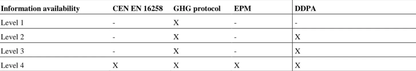
On levels 1-3 some information is missing or is allowed to change in terms of upcoming stops and/or consignments involved, whereas on level 4, all information required by the most information-demanding allocation methods considered in this paper, is available. Level 1 reflects, for instance, a scenario where only the addresses of the loading and unloading points (and not the distances between them) of the consignments are known, together with their weights and volumes. Along the transport route, the emissions from each unit of distance travelled can be directly estimated and allocated to the consignments currently inside the vehicle. Level 1 reflects the information requirements of the GHG protocol allocation method (see Table 2). On level 2, information about previously unloaded consignments is available (i.e. history data is available). On level 3, the entire route is known, however, the future loadings and unloadings are still unknown, apart from the unloadings of the consignments currently inside the vehicle. The transport weights during the latter part of the route are thereby also unknown (which affects the emission estimates). Level 4 reflects the information requirements of the CEN EN16258:2011 and EPM allocation methods (see Table 2). Levels 2-4 can all be applied by DDPA, since DDPA supports different levels of information availability (see Table 2). The allocation methods using level 4 employ different types of distance measurements; CEN EN16258:2011 recommends using great circle distances (as mentioned above), whereas EPM applies actual travelling distances, which is also recommended for DDPA.
Table 2 The information availability levels that the reference methods and DDPA works with Information availability CEN EN 16258 GHG protocol EPM DDPA
Level 1 - X - -
Level 2 - X - X
Level 3 - X - X
Level 4 X X X X
4.2
Information availability during transport versus after
Vehicle emission calculations based, for instance, on real-time measurements of fuel consumption, speed and acceleration/deceleration, all of which may be accessed directly from the vehicle, enable relatively precise emission estimations. If transport emissions can be locally allocated to the consignments at the time of unloading (i.e. emission shares are estimated during transport and assigned to consignments when they are unloaded), the emission shares can be computed and stored, based on the Intelligent Product concept (Meyer et al., 2009). The concept of Intelligent Products generally implies decentralised freight intelligence, i.e. some level of information processing and/or storage is implemented on, or close to, the products being transported, and is present throughout the whole transport. Intelligent Products also have the means to communicate. In this context, Intelligent Products can store information about the consignments (e.g. weigh and volume), which is needed by the allocation methods, as well as compute and store all emission shares during transport, from each individual transport leg. The total amount of emissions associated with a product can thereby be retrieved when the product reaches its final destination. The main benefits of this approach, in comparison to a more centralised configuration, might be that necessary interactions between different types of central information systems (which might have different interfaces etc.) are avoided. Data integrity and confidentiality may also benefit, since fewer intermediate actors are needed. The main disadvantage of this approach is, however, that in a dynamic transport planning system, only a limited amount of information might be available at the time of unloading, in terms of upcoming stops and/or consignments involved (see information availability levels 1-3). DDPA supports calculation and storage of emission shares at the time of unloading, even in a dynamic transport planning system; however, estimates are necessary. In a non-dynamic transport planning system, all stops and consignments involved in the route are known, and more precise emission estimates and allocations can thereby be obtained (see information availability level 4).
Emission estimations and allocations might also benefit from being performed after the route has ended, when the total amount of emissions caused by the entire transport may be more accurately estimated (using, for instance, real-time measurements on the actual fuel consumption from the entire route). In a dynamic transport planning system, information about the entire route and the consignments involved is not available until after the route has ended, which means that only at this point can the most accurate allocations be obtained. This type of solution discourages storing the emission share on
the physical products for practical reasons. For instance, the already unloaded products might be scattered by the end of the route and thereby hard to reach, e.g., transported further in another vehicle. However, even if emission shares are stored centrally, the time delay introduced may cause problems if the information is required before the route has ended. For instance, the products might already be placed for sale (or even sold) or they might have been disassembled. In practice, a combination of data from different sources might furthermore be needed to obtain all pieces of information necessary for the allocations, which may require interactions between different central information systems.
5. DDPA
5.1
DDPA with information availability level 4
DDPA has been developed from the idea that costs should respect the stand-alone costs of the consignments involved (as for EPM). Translating this idea to our particular situation has resulted in the following principle: emissions allocated to individual consignments should be influenced by the level of emissions that would be incurred if the consignment were sent by separate, dedicated transport.
Based on this principle, Eq. (1) has been developed, which allocates the emissions from the entire transport route based on distance and one limiting factor. In this paper, a transport route is considered ended when all consignments have been unloaded and any necessary repositioning has been performed.
Emissions allocated based on distance and one limiting factor:
Emc,l = Emtot * (𝐷𝐷𝑐𝑐 ∗ 𝐿𝐿𝑐𝑐,𝑙𝑙) / ∑𝑘𝑘∈𝑁𝑁(𝐷𝐷𝑘𝑘 ∗ 𝐿𝐿𝑐𝑐,𝑙𝑙) (1)
Emc,l = Emissions allocated to consignment c, based on distance and limiting factor l
Emtot = Total estimated emissions from transport route
Dc = Distance of a dedicated transport of consignment c
Lc,l = Quantity of limiting factor l of consignment c, e.g., physical weight or volume
N = All consignments involved in the transport route, forming a coalition
We use index c to denote one specific consignment, and index k to denote consignments in a sum.
The amount of total emissions caused by the entire transport route (Emtot) can be estimated using any of the methods
from literature (Boulter and McCrae, 2007; EEA, 2009; NTM, 2010). Ideally, the actual distance travelled should be used. Eq. (1) allocates the total amount of emissions from a transport route to individual consignments based on an approximation of their relative savings from being a part of the route. The equation is thereby more suitable for a route with several points of loading and unloading, in contrast to for instance the GHG protocol allocation method, which allocates emissions based only on the actual distance a consignment has travelled. Furthermore, emissions from the entire route, including prepositioning and repositioning transport, are distributed among the consignments according to the approximation of individual savings, since they are included in Emtot. As a consequence, Eq. (1) does not fulfil the
requirements of information availability levels 1-3.
Since we believe that the capacity of a vehicle may be limited by several factors, Eq. (2) has been developed, introducing a weighted combination of all relevant limiting factors (reflecting the relative significance of each limiting factor). For instance, one vehicle driving different types of consignments might be limited by weight and volume, whereas another vehicle driving light products only which never reach the weight limit, might be limited by the vehicle floor space only (e.g. number of pallets).
Emissions allocated based on distance and several limiting factors:
Emc = ∑ (𝛼𝛼∀𝑙𝑙 𝑙𝑙∗ 𝐸𝐸𝐸𝐸𝑐𝑐,𝑙𝑙) where (2)
∑ (𝛼𝛼∀𝑙𝑙 𝑙𝑙) = 1, 0 ≤ 𝛼𝛼𝑙𝑙≤ 1
Emc = Emissions allocated to consignment c, based on distance and all limiting factors
𝛼𝛼𝑙𝑙 = Weighted number between 0 and 1 reflecting the relative magnitude of the limiting factor l
Eqs. (1) and (2) represent DDPA when used with information availability level 4. In order to use DDPA with lower levels of information availability, some approximations must be made.
5.2
DDPA with information availability levels 2 and 3
Information availability level 2 reflects a scenario in which information about upcoming stops and consignments may be unreliable or unknown. The transport route might, for instance, change dynamically or additional loadings might occur at a stop. In order to use DDPA with this level of information, only the emissions caused by the route so far, in combination with the predicted future emissions from the consignments involved so far (inside the vehicle or already unloaded), are allocated. The future loadings of new consignments are ignored since we have no information about them. Instead, the weight and points of loading and unloading of the consignments currently inside the vehicle, as well as of those already
unloaded, are used to estimate the remaining emissions. Eq. (3) corresponds to Eq. (1), when applied to information availability level 2. Please note that only the consignments involved in the route so far are included.
Emissions allocated based on distance and limiting factor, with information availability level 2:
𝐸𝐸𝐸𝐸𝑐𝑐,𝑙𝑙𝑙𝑙𝑙𝑙𝑙𝑙𝑙𝑙𝑙𝑙 2 = (Emsofar + Emapprox) * (Dc * Lc,l) / ∑ (𝐷𝐷𝑘𝑘∈𝑆𝑆 𝑘𝑘 ∗ 𝐿𝐿𝑘𝑘,𝑙𝑙) (3)
𝐸𝐸𝐸𝐸𝑐𝑐,𝑙𝑙𝑙𝑙𝑙𝑙𝑙𝑙𝑙𝑙𝑙𝑙 2 = Emissions allocated to consignment c, at information availability level 2, based on distance and
limiting factor l
Emsofar = Estimated emissions from the distance travelled so far
Emapprox = Approximated emissions from the distance left, based only on the points of unloading of the
consignments currently on the vehicle
S = All consignments involved in the distance travelled so far (i.e. either inside the vehicle or previously unloaded), forming a coalition
Emapprox.and Emsofar can be estimated using the same methods as for Emtot. The estimated amount of emissions left
(ahead) (Emapprox.) is based on the route ending point as well as the unloading points of the consignments currently inside
the vehicle. This means that the estimation might be lower than the real value, since additional stops and consignments might be added later on. However, the divisor in Eq. (3), i.e. the sum of all consignment dedicated transport distances times their limiting factor quantity, will also be lower since only the consignments involved so far are included. The equation thereby provides an estimate based on the current state of the transport.
6. Simulation setup
We have developed a new discrete-event simulation program, written in Java, in which DDPA and the reference allocation methods have been implemented. The Network for transport and the environment (NTM) method has been selected to estimate transport emissions in the simulation program, since it represents a straightforward emission factor- and weight-based way of estimating emissions (NTM, 2010). The choice of method has little impact on our conclusions since we are only interested in evaluating emission allocations, not the actual amount of estimated emissions. However, some of the methods simulated under- or overestimate the total amount of emissions from a route, which means that the boundaries of the emissions that are allocated may differ between the methods. This aspect has to be taken into account when reading the simulation results.
NTM method estimates the emissions by using the following set of equations.
Fuel consumption per distance unit of a vehicle (NTM, 2010):
𝐹𝐹𝐹𝐹𝑥𝑥,𝑦𝑦𝐿𝐿𝐿𝐿𝐿𝐿 = 𝐹𝐹𝐹𝐹𝑥𝑥,𝑦𝑦𝑙𝑙𝑒𝑒𝑒𝑒𝑒𝑒𝑦𝑦 + (𝐹𝐹𝐹𝐹𝑥𝑥,𝑦𝑦𝑓𝑓𝑓𝑓𝑙𝑙𝑙𝑙 – 𝐹𝐹𝐹𝐹𝑥𝑥,𝑦𝑦𝑙𝑙𝑒𝑒𝑒𝑒𝑒𝑒𝑦𝑦) * LCUweight (4)
LCUweight = Load Capacity Utilization defined as [cargo physical weight/max weight capacity]
𝐹𝐹𝐹𝐹𝑥𝑥,𝑦𝑦𝐿𝐿𝐿𝐿𝐿𝐿 = Fuel consumption at load capacity utilization LCU, road type x and vehicle type y
Total emission of substance i for driving on road type x with a vehicle of type y (NTM, 2010):
𝐸𝐸𝐸𝐸𝑖𝑖,𝑥𝑥,𝑦𝑦𝐿𝐿𝐿𝐿𝐿𝐿 = EFi, x, y * 𝐹𝐹𝐹𝐹𝑥𝑥,𝑦𝑦𝐿𝐿𝐿𝐿𝐿𝐿 * Dist (5)
𝐸𝐸𝐸𝐸𝑖𝑖,𝑥𝑥,𝑦𝑦𝐿𝐿𝐿𝐿𝐿𝐿 = Emissions of substance i for driving on road type x with vehicle type y and load capacity utilization
LCU
EFi, x, y = Emission factor for substance i, dependent on road type x and vehicle type y
Dist = Distance travelled (on road type x with vehicle type y)
The values used for 𝐹𝐹𝐹𝐹𝑥𝑥,𝑦𝑦𝑓𝑓𝑓𝑓𝑙𝑙𝑙𝑙 and 𝐹𝐹𝐹𝐹𝑥𝑥,𝑦𝑦𝑙𝑙𝑒𝑒𝑒𝑒𝑒𝑒𝑦𝑦 are acquired from the Heavy Goods Vehicle (HGV) fuel consumption data presented in the NTM report (in terms of liters per kilometer) (NTM, 2010). They are dependent on vehicle type and the type of road used (motorway, rural or urban), including the condition of the road traffic (free flow, saturated or heavily congested). LCUweight is calculated as the weight of all consignments in the vehicle divided by the maximum weight
capacity for the vehicle in question. The emission factors are also acquired from the NTM report, in which they are given in terms of gram per liter fuel for each emission substance.
The emission estimations used in the simulations are based on a Euro IV type lorry with trailer, using diesel (the same type of vehicle as used in a calculation example in the NTM report). The lorry is assumed to have unlimited load-weight and load-volume capabilities, in order to preserve random distribution behaviour. Moreover, the vehicle is assumed only to be travelling on free-flow roads. Again, the choice of assumed vehicle does not affect our conclusions since we are only interested in emission allocations.
The program simulates transport routes comprising 3-8 different cities in Sweden (including starting and ending nodes), randomly selected from a set of 17 cities. This random selection is weighted according to the sizes of the cities. The starting node is randomly selected (with unweighted distribution), and for simplicity we assume that the ending node is the same as the starting node. Actual travelling distances between the cities, based on information from Google Maps, are used in the simulations. A transport route is found by applying an algorithm for the Travelling Salesman Problem, and if two different shortest routes can be found with equal total distances, they are each selected with equal probability. Exactly 10 consignments are loaded and unloaded during the transport. For each consignment, a loading point and an unloading point are randomly selected from the cities involved in the route (including the starting and ending nodes). These selections are also weighted according to the sizes of the cities and they are constrained by the order of the stops visited. Finally, any city involved in the route but without any consignment activities (i.e. neither loadings nor unloadings occur in the city), is removed from the transport route.
The aim of using these settings has been to simulate a variety of different transport requirements, corresponding to realistic transport scenarios (involving both loadings and unloadings within the same route, or reflecting pure pick-up or delivery routes). By investigating information published by transport companies operating in the south of Sweden, we have found that the simulated routes reflect many of the companies’ transport routes, i.e. they apply routes with several loadings and unloadings, or pure pick-up or delivery routes, and the number of consignments often correlates to the size of a city. The reason for limiting the number of consignments in the simulations is that we want to keep the processing time of the EPM allocation method reasonable. The EPM processing time increases with the number of consignments (see section 7.2) and we have not seen any significant changes to the results when simulating more consignments, in small scale tests.
Weight and volume are regarded as the limiting factors of the vehicle in the simulations. The weight and volume of each consignment are determined by randomly selected values between 1-5 ton and 1-5 m3, and weight and volume are
considered as equally important, i.e. α1 = α2 = 0.5. The reason for selecting these values is that we want to show how
DDPA behaves in the long run when the impacts from weight and volume even out. The effects of having different impacts from weight and volume are also illustrated, by simulating an individual transport route. The vehicle is driven on three different types of roads; 95% motorway, 4% rural roads and 1% urban roads (again reflecting the calculation example in the NTM report). This distribution has only been used when fuel consumption based on the NTM tables has been estimated in these simulations.
Only one type of emission is estimated, namely CO2, since we are only interested in the results of the allocations. Other
types of emissions can easily be implemented using the calculation methods presented by NTM (NTM, 2010), but since they will not further affect the outcome of the simulations, they have been omitted. Since CO2 emissions depend on fuel
carbon content, and not, for instance, on road type, the emission factors used in these simulations will be constant (which would not be the case for some other types of emissions).
The results are presented as emissions allocated to each consignment, in combination with relative savings. The relative saving (RS) of consignment (participant) i is defined as the difference between the stand-alone cost (c({i})) and the allocated cost (yi) of that participant, in relation to the stand-alone cost (Frisk et al., 2010):
𝑅𝑅𝑅𝑅 = 𝑐𝑐({𝑖𝑖})− 𝑦𝑦𝑖𝑖 𝑐𝑐({𝑖𝑖}) = 1 -
𝑦𝑦𝑖𝑖
𝑐𝑐({𝑖𝑖}) (6)
As can be seen, if the cost allocated to participant i equals the stand-alone cost of participant i, the relative saving becomes zero. In this paper, costs correspond to emissions. We have chosen to present the allocated emissions with the relative savings because transport actors involved in a transport route seem, in general, to want the relative savings to be as similar as possible for all actors (Frisk et al., 2010). In addition, the relative savings effectively illustrate both how the methods affect the allocated emissions in different situations and the differences between the selected allocation methods.
7. Simulations without compensation factors
The first part of this section presents the results from simulating only one transport route. The aim of this simulation is to explain and illustrate how the allocation methods behave, i.e. it illustrates the ideas behind the methods. The second part of this section presents the results from simulating 100 000 transport routes, illustrating how the methods allocate emissions in the long run. In order to validate the findings, we have repeatedly simulated one route, 10 000 routes and 100 000 routes and compared the results. These simulations exhibit the same behaviours as presented in this paper.
7.1
Results and analysis of simulation of one transport route
Running the simulation program for one transport route resulted in the stops and consignments presented in Figure 1 and Table 3. Note that the dedicated transport distance related to a consignment consists of a route beginning with the starting node (in this case Landskrona), and continuing to the points of loading, unloading and finally to the ending node (in this case Landskrona). Table 4 shows the CO2 emission allocation results from all simulated allocation methods. DDPA is
simulated with information availability levels 2 and 4. When level 2 is simulated, the allocations are calculated and dedicated to the consignments being unloaded at each stop. The reference allocation methods are always simulated with their respective information requirements as presented above.
Table 3 Simulated consignments
No. Loading point Unloading point Dedicated transp. dist. (km) Weight (ton) Volume (m3)
1 Helsingborg Malmö 135.4 5 3 2 Helsingborg Malmö 135.4 5 3 3 Malmö Kristianstad 250.7 2 2 4 Helsingborg Malmö 135.4 1 2 5 Malmö Kristianstad 250.7 5 1 6 Malmö Kristianstad 250.7 4 2 7 Malmö Landskrona 87.2 1 5 8 Helsingborg Kristianstad 270.6 4 2 9 Malmö Landskrona 87.2 2 2 10 Landskrona Malmö 87.2 1 4
Table 4 Simulation results; one transport route CEN EN 16258:2011, information level 4 GHG protocol, information level 1 EPM, information level 4 DDPA, information level 4 DDPA, information level 2 No. CO2 (g) Saving (%) CO2 (g) Saving (%) CO2 (g) Saving (%) CO2 (g) Saving (%) CO2 (g) Saving (%)
1 30212 65.20 14790 82.96 19134 77.96 26161 69.87 46977 45.89 2 30212 65.20 14790 82.96 19134 77.96 26161 69.87 46977 45.89 3 19949 87.04 11042 92.83 33919 77.96 25450 83.46 25450 83.46 4 6042 92.67 5766 93.01 18173 77.96 10974 86.69 19196 76.72 5 49873 68.59 15183 90.44 34994 77.96 33250 79.06 33250 79.06 6 39899 74.61 15873 89.90 34636 77.96 35713 77.28 35713 77.28 7 3559 93.30 55872 -5.14 11386 77.96 14991 71.79 14991 71.79 8 42024 75.51 26903 84.32 37811 77.96 38547 77.53 38547 77.53 9 7117 86.79 45523 15.51 11223 77.96 8852 83.57 8852 83.57 10 3559 93.30 26706 49.74 12037 77.96 12350 76.76 21380 59.77 Sum: 232448 232448 232448 232448 291332
The results of the simulations of DDPA, when used with information availability 4, are in line with the ideas behind the new method. Consignments with longer dedicated transport and larger shares of volume and weight, receive higher amounts of emissions (see, e.g., consignment no. 8). Consignments with a low total sum of weight and volume achieve high relative savings since they benefit from sharing the transport emissions with bigger and heavier consignments (see, e.g., consignment no. 4). As a secondary effect, relatively heavy consignments also receive some minor benefits from the allocation method in comparison to consignments of relatively large volumes, since the dedicated transport for these former consignments cause slightly higher emissions. This means that a consignment with a high weight but low volume achieves higher savings in comparison to a consignment with a high volume but low weight; as expected (compare, e.g. relative savings of consignments nos. 5 and 7). On the other hand, in this particular simulation, the total weight of all consignments is 30 ton and the total volume is 26 m3. A higher volume thereby has slightly more impact on the allocated
amount of emissions than a higher weight (compare, e.g., the emissions allocated to consignments nos. 5 and 6). All this is in line with the design, as are the varying relative savings (which are further discussed below).
Table 4 also shows that DDPA, when used with information availability level 2, allocates more than the total amount of emissions (which is 232448g). This error arises due to the lack of knowledge about future loadings and unloadings during the first part of the route, and it can be reduced by using compensation factors (as will be shown). In this example, consignments nos. 1, 2, 4 and 10 receive far too high emission shares in comparison to when the method is used with
Figure 1 Transport route used in the initial simulation: Landskrona - Helsingborg - Malmö - Kristianstad - Landskrona
Kristianstad
Landskrona 27.4 km Helsingborg 64.4 km Malmö
96 km 111.1 km
First and last stop
information availability 4. The reason for this is that when these consignments are unloaded in Malmö, the system has no knowledge of any additional consignments, and the emissions are therefore poorly shared. The lack of knowledge about future loadings and unloadings often reduces the number of known stops ahead. This shortened route leads to an emission reduction which may compensate for the increased allocations given by the lack of knowledge of other consignments to share emissions with. However, the results show that in general, the more information we have, the better the results can be obtained.
In CEN EN16258:2011, the total amount of emissions from the entire route is allocated (including prepositionings and repositionings), and all consignments with the same loading and unloading points receive the same emission shares, weighted on consignment weight. Table 4 shows that consignment no. 4 has 1/5 of the weight of consignments nos. 1 and 2 but the same loading and unloading points, and it thereby receives 1/5 of the emissions of consignments nos. 1 and 2. The highest amount of emissions is allocated to consignment no. 5, which has maximum weight and the second longest distance between the points of loading and unloading.
Table 3 and Figure 1 show that the particular route and consignments simulated do, by coincidence, not include empty prepositioning and repositioning transport, i.e. both loading and unloading take place at the starting/ending node. In the GHG protocol results, the total amount of emissions from the entire route is therefore allocated. This would not have been the case if such empty transport been present (see section 7.2). Furthermore, in this simulation, consignment no. 7 receives negative relative savings. This is because consignment no. 7 is allocated a share of emissions from a relatively long distance, although the dedicated transport distance is relatively short. The consignment also has a relatively high sum of weight and volume. Negative relative savings are further discussed in the next section.
Finally, Table 4 also shows that relative savings vary for all methods except EPM. This result is as expected since EPM aims for equal relative savings allocations in the individual case, whereas the others do not. Taking only relative savings into account, as EPM does, means that only one of the limiting factors, weight, has been respected (whereas DDPA also takes the consignment volume into account). Furthermore, the consignment weights have less influence on the allocations, in comparison to DDPA (since relative savings are only partly affected by weight). Had some other measure, taking all limiting factors into account, been used instead of relative saving, then the corresponding DDPA results column would show more equal values.
The example run and description above demonstrates the characteristics and qualities of DDPA, listed in Table 1. However, the effects of individual consignment with distant points of loading/unloading in relation to other consignments, and the effects of the limiting factors can be further illustrated by the use of transport scenarios. For this purpose, we have defined two different scenarios:
1. Distribution round where all consignments are loaded at a terminal, 5 km from the starting node. Nine of the consignments are unloaded at stop A, 10 km from the route starting node, and the remaining consignment is unloaded at stop B, 20 km from the starting node. The route ends at the starting node. For simplicity, all stops are placed on a straight line from the starting/ending node. All consignments have equal weight (2 ton) and volume (2 m3).
2. Distribution round where all consignments are loaded at the route starting node and delivered to the stops A, B, C, D, E, F, G, H, I, J in that order, i.e. one consignment is delivered at each stop. The route ends at the starting node. All stops have equal distance to the starting node (10 km), i.e. all consignments have the same dedicated distance. Nine of the consignments have equal weight (1 ton) and volume (1 m3), and the last
consignment, unloaded at stop J, has twice the volume (1 ton, 2 m3).
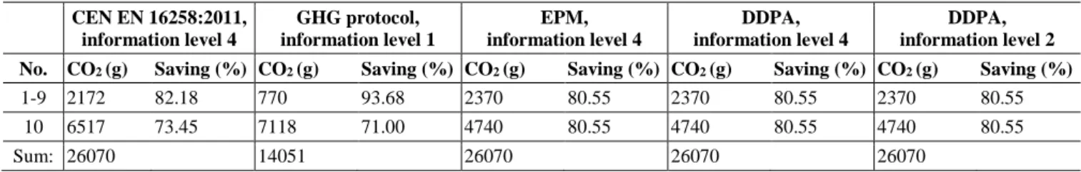
Scenario 1 aims to illustrate the effects of having one individual consignment with a distant point unloading in relation to the other consignments’ points of unloading, whereas scenario 2 is focussed on the effects of having one larger individual consignment in relation to the other consignments’ size. In contrast to the example run described above, both scenarios illustrate pure distribution rounds (or collection runs, which will give the same results). Table 5 shows the results of allocation in scenario 1.
Table 5 Allocation results; scenario 1 CEN EN 16258:2011, information level 4 GHG protocol, information level 1 EPM, information level 4 DDPA, information level 4 DDPA, information level 2 No. CO2 (g) Saving (%) CO2 (g) Saving (%) CO2 (g) Saving (%) CO2 (g) Saving (%) CO2 (g) Saving (%)
1-9 2172 82.18 770 93.68 2370 80.55 2370 80.55 2370 80.55
10 6517 73.45 7118 71.00 4740 80.55 4740 80.55 4740 80.55
Sum: 26070 14051 26070 26070 26070
As can be seen, DDPA allocates twice as much emissions to the last consignment, due to the doubled distance to the route starting and ending nodes, while it maintains the same relative savings as the rest of the consignments. Since all consignments are known from the beginning of the route, DDPA performs the same way for information availability levels 2 and 4. EPM finds the same solution. However, the GHG protocol allocates all emissions from the terminal to stop A, equally to all consignments, whereas all emissions from stop A to stop B are allocated to the last consignment. The rest of the emissions (i.e. to/from the ending/starting nodes) are neglected. CEN EN16258:2011 focusses on the distance between
loading and unloading only, which means that the consignment unloaded at stop B get a relatively higher share of the total emissions. The relative savings, which respect the stand-alone cost, is thereby lower.
Table 6 shows the results of allocation in scenario 2.
Table 6 Allocation results; scenario 2 CEN EN 16258:2011, information level 4 GHG protocol, information level 1 EPM, information level 4 DDPA, information level 4 DDPA, information level 2 No. CO2 (g) Saving (%) CO2 (g) Saving (%) CO2 (g) Saving (%) CO2 (g) Saving (%) CO2 (g) Saving (%)
1 7542 38.12 735 93.97 7542 38.12 7199 40.93 7199 40.93 2 7542 38.12 1530 87.44 7542 38.12 7199 40.93 7199 40.93 3 7542 38.12 2400 80.31 7542 38.12 7199 40.93 7199 40.93 4 7542 38.12 3364 72.40 7542 38.12 7199 40.93 7199 40.93 5 7542 38.12 4451 63.48 7542 38.12 7199 40.93 7199 40.93 6 7542 38.12 5708 53.17 7542 38.12 7199 40.93 7199 40.93 7 7542 38.12 7212 40.82 7542 38.12 7199 40.93 7199 40.93 8 7542 38.12 9113 25.22 7542 38.12 7199 40.93 7199 40.93 9 7542 38.12 11758 3.53 7542 38.12 7199 40.93 7199 40.93 10 7542 38.12 23137 -89.83 7542 38.12 10627 12.81 10627 12.81 Sum: 75418 69409 75418 75418 75418
As in scenario 1, DDPA behaves the same way for information availability levels 2 and 4 since all consignments are known from the beginning of the route (they are loaded at the starting node). All consignments have equal weight and dedicated distance, and therefore, DDPA allocates half of the total amount of emissions equally between the consignments. As for the other half, the last consignment with twice the volume receives 1/11 more emissions since it has 1/11 more volume than the rest (which corresponds to 75418/2/11 = 3428). The relative savings for the last consignment is lower than for the other consignments since the relative savings formula (Eq. 6) does not include volumetric aspects. As before, EPM finds an optimal solution with respect to relative savings. CEN EN16258:2011 allocates the same way as EPM since all consignments have equal weight and distance between their points of loading and unloading. The GHG protocol allocates a relatively small amount of emissions to the consignment unloaded first, since its transport distance is short and the corresponding emissions are shared with all the other consignments. The last consignment receives a relatively large amount of emissions since its transport distance is long and since the number of consignments to share the emissions with is decreased along the route. The emissions to the ending node is neglected.
7.2
Results and analysis of simulations of 100 000 transport routes
In order to investigate the behaviour of DDPA in the long run, we have simulated a large number of transport routes. Table 7 shows the mean values from 100 000 simulations, where each simulation involved a transport route of 10 consignments. The consignments have been ordered according to the point of unloading, since we want to show how DDPA allocations affect consignments being unloaded at an early stage and at a later stage of the transport route, respectively. The consignment being unloaded first was placed at the top of the results list and the consignment unloaded last was placed at the bottom.
EPM investigates the cost of each possible coalition. Since the number of possible coalitions quickly increases with the number of participants (for n participants, the number of coalitions is 2n – 1 – n (Frisk et al., 2010)), the size of the
optimisation model increases dramatically. With size, the computational time also increases. Since a simulation of 100 000 routes using EPM requires excessive simulation time, EPM has been excluded from the simulations in this section. Moreover, since the results of DDPA, when used with information availability level 4, show a nearly equal relative saving, these results also indicates the results of EPM.
Table 7 Simulation results; 100 000 transport routes CEN EN 16258:2011
with info. level 4
GHG protocol with info. level 1
DDPA with info. level 4
DDPA with info. level 2 No. CO2 (g) Saving (%) CO2 (g) Saving (%) CO2 (g) Saving (%) CO2 (g) Saving (%)
1 17041 79.05 14354 76.94 17238 78.96 32274 55.16
2 17641 79.96 11764 82.43 18232 78.96 23359 72.39
3 17461 80.08 11264 82.95 18089 78.91 20614 75.87
4 17023 80.10 11292 82.41 17592 78.90 19006 77.21
6 16006 79.85 12234 79.78 16337 78.86 16810 78.28 7 15497 79.38 13258 77.04 15522 78.82 15761 78.52 8 14843 78.78 14599 73.25 14535 78.83 14630 78.71 9 14018 77.52 17257 64.68 13130 78.80 13155 78.77 10 12675 75.61 23906 41.70 11022 78.89 11022 78.89 Sum: 158725 141555 158725 184497
In the long run, DDPA aims for equal relative savings on average (when specific transport requirements, e.g., weight and volume, even out). Table 7 shows that when used with information availability level 4, DDPA achieves almost equal relative savings. When the method is used with information availability 2, consignments unloaded at the beginning of a route receive, on average, a higher amount of emissions, due to lack of knowledge about consignments to share emissions with (as in Table 4). Since the error follows a pattern (see last column in Table 7), it may be reduced by lowering the initial allocations by some compensation factor. For CEN EN16258:2011 and the GHG protocol, the relative savings vary on average, though CEN EN16258:2011 shows less variation than the GHG protocol. The experiences gained from the simulations of the GHG protocol and the CEN EN16258:2011 allocation methods are that the relative savings do not follow a pattern as they do for DDPA. As a consequence, compensation factors will be of little use in the GHG protocol and CEN EN16258:2011 methods.
CEN EN16258:2011, EPM and DDPA used with information availability level 4, all fulfil the efficiency property (Tijs and Driessen, 1986), which means that the emissions from the entire route are divided between the consignments. The total amount of emissions is thereby shown by the corresponding sums in Table 7. DDPA used with information availability level 2 does not fulfil the efficiency property due to the over-allocations to the early unloadings. The GHG protocol does not fulfil the efficiency property either since it disregards empty prepositionings and repositionings.
In the GHG protocol simulations, the consignments being unloaded last receive the highest emission shares, on average (see Table 7). This can be explained by the fact that there is a greater possibility that these consignments have travelled a longer distance in total, following the route through more intermediate stops, than those being unloaded at the beginning of the route.
A weakness of DDPA is that in a few cases, relative savings will be negative. This means that some consignments involved in a transport route receive more emissions than if they were transported in separate, dedicated transports, which may be considered as unfair (see section 2). In our simulations, this occurs for < 0.0004% of the consignments when information availability level 4 is used. The negative relative savings are caused by consignments with exceedingly dominating weight and volume (in comparison to the other consignments in a route). In reality, negative relative savings may also occur if the relation between the emissions and the distances is very uncorrelated. However, if we would only use the dedicated transport distance part of DDPA and disregard the fact that the emissions are dependent on weight, the relative individual savings would be the same for all consignments. Negative relative savings occur for < 0.023% of the consignments in the CEN EN16258:2011 simulations and for < 4.6% of the consignments in the GHG protocol simulations. The relatively high number for the GHG protocol reflects the effects of the GHG protocol being primarily designed for transport with single points of loading and unloading, and that emissions to distant loading and unloading points are allocated between the consignments being co-loaded to these stops. The minimum negative saving is always less negative, when they appear, for DDPA than for the CEN EN16258:2011 and the GHG protocol allocations. For DDPA when used with information availability level 2, negative relative savings occur for < 0.6% of the consignments, due to the lack of knowledge about future loadings and unloadings.
8. Simulations with compensation factors
The average error produced by DDPA when used with information availability level 2, in relation to when it is used with information availability level 4, as shown in Table 7, may be reduced by introducing compensation factors. Such compensation factors represent, in principle, a prediction of the upcoming part of the route, as well as the corresponding loadings and unloadings.
We have explored the results of the previous simulation of 100000 routes, with particular focus on the allocation results at each stop number. The reason for this is that we want to capture and reduce the average systematic errors received by the early unloadings (last column of Table 7), by identifying compensation factors for all consignments unloaded at the same stop number. Table 8 shows the average amount of emissions allocated to the consignments being unloaded at stop number (s): 2, 3, 4 etc. Since the relative knowledge about the rest of the route is usually higher at any point in a route with few stops than at the corresponding stop number in a route with many stops, the amounts of over-allocation usually increases with route size (r), as can be seen in Table 8. For instance, at the third stop of a route of size 3, all loadings and unloadings are known and no over-allocation is present. At the third stop of a route of size 8, on the other hand, little is known about future loadings and unloadings, which causes increased over-allocation. Note that the sums of all mean allocations in Table 8 do not correspond to the sums in Table 7, since they are based on different types of mean values (with different denominators).