Study on the flow of water through non- submerged vegetation

Full text

(1)Hydrology Days 2005. Study on the flow of water through nonsubmerged vegetation Nehal L1 Water Conservancy and Hydropower Engineering College. Hohai University. Nanjing, China.. Yan Zhong Ming1 Water Conservancy and Hydropower Engineering College. Hohai University. Nanjing, China.. Abstract. Vegetation is an important feature of many rivers. Vegetation along rivers produces high resisatnce to flow and, as a result, has a large impact on water levels in rivers and lakes. This paper investigates the effects of instream-unsubmerged vegetation (such as the reed-similar Kalmus) on flow resistance and velocity distributions. Artificial vegetation is used in the experimental study to simulate the Acorus Calmus L. Experimental tests have shown that resistance depends strongly on vegetation density and that the Manning resistance coefficient varies with the depth of flow. A simplified model based on concepts of drag is developed to evaluate the roughness coefficient (Manning’s n) for unsubmerged vegetation. In vegetated channels the overall flow resistance is influenced significantly by the distribution pattern of the vegetated beds. Within vegetation, the mean velocity decreases with flow for which the vegetative roughness increases with decreasing velocity and vertical turbulent transport of momentum is negligible as demonstrated by experiments.. 1. Introduction Vegetation is an important feature of many rivers, providing habitat for other aquatic organisms and enhancing amenity value for people. It is a key element in river functioning, through a three way, mutual feedback relationship with channel morphology and hydraulics (James et al. (2001)): Vegetation and channel form determine hydraulic conditions for a given discharge; hydraulic conditions and channel form define habitat for vegetation establishment and growth; vegetation and hydraulics determine channel form by controlling the movement, trapping, and storing of sediment. Environmental management of rivers requires understanding and predictive capability of these processes, and in particular the influence of vegetation on flow resistance. There has been increasing interest and research in floodplain management of rivers and natural waterways for a wide range of civil and water resource activities. In areas where flow occurs through vegetation, the characteristics of the flow are largely determined by the type and density of vegetation as well as the depth and velocity of the flow. The flow resistance problem can be classified into two categories: flow over short, submerged vegetation and flow in tall, nonsubmerged vegetation. For flow of water through nonsubmerged vegetation, previous investigations resulted in a series of relationships with only a very limited range of application (i.e., for a very low range of velocity where deflection of vegetation is negligible and for. 1. Hohai University. 1, Xikang road. Foreign student building, room N 213. Nanjing, 210098. China. Tel: (0086)-25-83789853; e-mail: laounia2001@yahoo.fr ©Hydrology Days. 170.

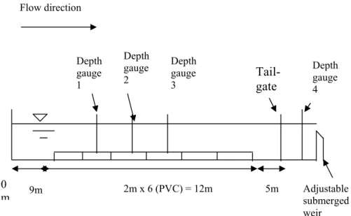
(2) Study of flow through non-submerged vegetation. canopies with low vegetation density). Mostly, practitioner used photographs and tables to estimate Manning’s n values (Chow 1959; Barnes 1967). Nonsubmerged vegetation along rivers and floodplains consumes a great amount of energy and momentum from the flow, and is often found to be in the region with the most roughness. Estimation of the roughness coefficient in this region is a major factor in construction of river stage- discharge curves, especially during flood events. The relationship between flow velocity (and hence discharge) and flow depth (and hence area of inundation) in rivers is commonly established through a resistance relationship, such as Manning’s equation, i.e.: U= n-1 R2/3 S1/2 (1) in which U is the average velocity, R is the hydraulic radius, S is the channel slope, and n is the Manning resistance coefficient. Application of this equation requires knowledge of an appropriate value for n, which depends on channel geometry, substrate, vegetation and flow conditions. Patryk and Bosmajian (1975) developed a quantitative procedure for predicting the Manning’s n value of nonsubmerged vegetations. The analytical results showed that the n value increased as depth if the vegetation density remained relatively constant with flow depth. Turnel and Chanmeesri (1984) measured the resistance coefficient of wheat vegetation under nonsubmerged conditions. They found that the resistance coefficient per unit length Cd decreases as the water depth increases. Chiew and Tan (1992) published their field observation on the resistance of nonsubmerged grass to water flow. Their research showed that the flow resistance was independent of water depth. Shen and Chow (1999) used horse hair in channel to simulate nonsubmerged vegetation, the experiment results showed that the flow resistance decreases as the water depth increases in turbulent flow. The different results above are perhaps caused due to the different density and kinds of vegetation in their research. It also means that the effect of nonsubmerged vegetation on flow resistance is not clear yet. It needs to further study. The Acorus Calmus L is a kind of typical nonsubmerged vegetation. It is widely planted in river or wetland because of its function of improving water quality and economy. But few researches have been done on the effects of theses plants on the flow. In this paper, the Acorus Calmus L is chosen to model vegetation to study its effects on water flow.. 2. Laboratory experiments The tests were conducted in a 26m long, 0.7m height and 0.5m wide rectangular, glass-walled flume. The slope of the flume was fixed at 0.07692%. Discharge was measured with a submerged weir at the end of the flume, and uniform flow was ensured by the adjustment of a tailgate at the downstream end. Flow depths were measured with two depth gauges at 12m and 16m (Fig. 1); the bed of the flume (study area) was roughened by a 12 m long and 2cm thick layer of PVC.. 171.

(3) Nehal and Yan Zhong Ming Flow direction. Depth gauge 1. 0 m. 9m. Depth gauge 2. Depth gauge 3. 2m x 6 (PVC) = 12m. Tailgate. 5m. Depth gauge 4. Adjustable submerged weir. Figure 1. Experimental set-up in the flume without vegetation. The vegetatedbed test facilities were equal but with vegetation mounted in the PVC layer (long- view; not to scale).. For the tests without vegetation, a fixed set of 8 discharges was used for the study. The uniform flow depth was measured at the equilibrium condition. For the vegetated bed (Fig. 3), a longitudinal section of artificial vegetation selected to simulate Acorus calamus L, was installed over a length of 12 m (study area see Fig. 1). The model vegetation was about 50cm - 60cm height. Each plant consisted of six blades of width w=1.7cm – 1.9cm, bundled to a basal stem of an average diameter 1.15cm and average height 9.12cm. The blades were made from plastic. The morphology of a single plant is shown in Fig. 2. The plants were arranged in a staggered pattern, with longitudinal and transverse spacing of 15 cm, 30cm and 45cm, by sticking the upper end of the plant into drilled holes. Velocity measurements were made with a 3-D Acoustic Doppler Velocimeter (ADV). For the four densities (280, 240, 60 and 40plants) the velocity distribution was measured at several points in the vertical.. Figure 2. The morphology of a single plant.. Figure 3. Experimental facilities for vegetatedbed test.. 172.

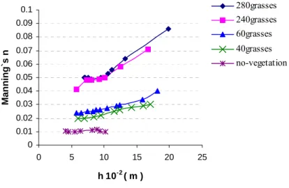
(4) Study of flow through non-submerged vegetation. 3. Theoretical considerations Drag is generated when a fluid moves through vegetation. The drag creates velocity gradients and eddies that cause momentum losses. These losses are significant for a wide range of flow conditions, and existing techniques for the prediction of resistance do not take these into account, leading to under predictions of resistance. Because vegetative drag can have a profound effect on the velocity and, thus, the water surface elevation, any expression of the flow conditions in a vegetated channel must include drag. A relation for unsubmerged vegetation can be formulated from the principle of conservation of linear momentum. Following a derivation similar to that for the de Saint Venant Equation, the sum of the external forces in a control volume (CV) is equated to the rate of change of linear momentum. Equating the slope term in Eq. (A10) to the slope term in Manning's Equation Eq. (1), a relation for Manning's n is established as: 1/ 2. ⎡C A ⎤ n=R ⎢ d d⎥ (2) ⎣ 2g ⎦ Where: n is the Manning resistance coefficient; R is the hydraulic radius, g is a gravitational constant; Cd is the drag coefficient; Ad = ∑Ai /A∑x is the vegetation density per unit channel length, Ai is the projected area of the ith plant in the streamwise direction and A is the cross sectional area of the flow. Eq. (2) requires an estimate of the drag coefficient Cd and the corresponding vegetation area. 2/3. 4. Flow through unsubmerged vegetated- beds A series of laboratory experiments have been carried out to investigate the influence of unsubmerged vegetation density and flow depth on the resistance imposed by vegetation. The roughness of the glass walls is negligible compared to the roughness of bottom. Hence, the flume was assumed to be very wide. Thus for the calculations, the water depth h was used instead of hydraulic radius R. The measured water depths and discharges for the non- vegetated and vegetated bed are plotted in Fig. 4, and the calculated roughness coefficient, n, is plotted against the flow depth in Fig. 5:. 0 .0 3 5. 0 .0 2 5 0 .0 3. 0 .0 1 5 0 .0 2. 0. vegetatedbed (280grass) vegetated bed (240grass) vegetated-bed (60grass) vegetatedbed(40grass). 0 .0 0 5 0 .0 1. -2. h 10 (m). non- vegetated bed 24 22 20 18 16 14 12 10 8 6 4 2 0. Q (m 3 s -1). Figure 4.. Water depth- discharge relationship for different vegetation densities. 173.

(5) Nehal and Yan Zhong Ming. 0.08. 280grasses 240grasses 60grasses. 0.07. 40grasses. 0.06. no-vegetation. 0.1. Manning`s n. 0.09. 0.05 0.04 0.03 0.02 0.01 0 0. 5. 10. 15. 20. 25. h 10-2 ( m ). Figure 5. Variation of roughness coefficient with flow depth through vegetation. Fig. 4 shows that the water depth increases with discharge in channels without vegetation, and the measured water depth agree with the computed values using an n=0.011. Manning’s n doesn’t change with the increase in water depth (Fig. 5), it is approximately constant, varying only between 0.010 and 0.011; which is equal to the value of n expected and used in the calculations. The relationship between flow depth (or stage) and discharge depends significantly on the vegetation density (Fig. 4); as the grasses density increases, the water depth increases. It is clear that the distribution pattern of the grasses has a significant effect on the overall resistance. The curves for the four patterns show that creating additional boundaries to the clear channel area, by separating them with grasses significantly increases resistance. The close correspondence between the curves for 280 and 240grasses is explained by the small difference between the two densities. Manning’s n is calculated from Eq. (2). Manning’s is clearly related to the plants density, it also varies with flow condition (Fig. 5) far more than in unvegetated channels. It is clear that the vegetative roughness increase with water depth. This shows that not only does the presence of grasses increase Manning’s substantially and that this depends on the pattern, but also Manning’s varies with flow depth. The values for the 4th density (40grasses) are consistently lower than for the 1st density (280grasses). In vegetated channels n has been found to be strongly correlated to the product UR, but practical application of this relationship is unsatisfactory. Apart from the undesirability of an equation for velocity including a coefficient which itself depends on velocity, the same value of UR may be obtained from different values of U and R, and the relationship is not independent of slope (Smith et al. (2001)). The difficulty arises because Manning’s equation, and the other similar resistance equations were developed for, and strictly applies only to, situations where flow is controlled 174.

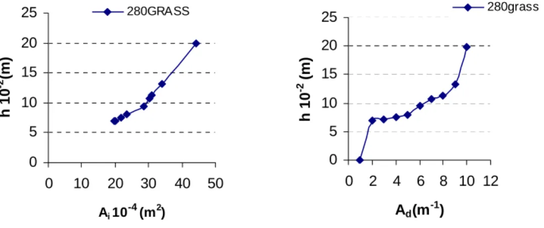
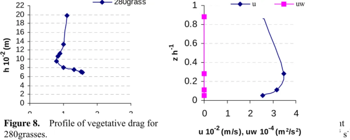
(6) Study of flow through non-submerged vegetation. by boundary resistance. The dominant control in vegetated channels arises from stem drag, which is applied through the flow depth and not just at the boundary. The projected area of an individual plant blocking flow and the vegetation density are calculated approximately and are plotted against water depth for the case of 280 plants, in Fig. 6 and 7 respectively. It is clear that the water depth increase with the projected area of plants blocking the flow in the four cases.. 280GRASS. 25 20. 20 h 10-2 (m). h 10-2(m). 280grass. 25. 15 10. 15 10. 5. 5. 0. 0 0. 10. 20. 30. 40. 0. 50. 2. 4. 6 8 10 12. Ad (m -1). Ai 10-4 (m 2). Figure 6. Variation of vegetation projected area with flow depth.. Figure 7. Vegetation density profile. The increase in vegetation density is attributed to increased leaf density, with height for the measured water depths. The drag coefficient is calculated using Eq. (A10) and is plotted against water depth in Fig. 8. Fig. 8 shows that over the lower half of the plant, the drag coefficient Cd increases towards the bed, reflecting the increasing importance of viscous effects. Above the bed, the unsubmerged plant produces a constant value of Cd ≈1. Mean velocities (u, v, w) corresponding to the streamwise (x), lateral (y), and vertical (z) directions, respectively were measured using threedimensional acoustic Doppler velocimeter (ADV). And the ADV data were analyzed using WinADV program. Profiles of mean velocity and Turbulent stress for the case of 280grasses are shown in Fig. 9 with a discharge 0.0049m3/s. From Fig. 9 two parts could be distinguished: the stem part where the velocity increases, and the leaf part where the velocity decreases slowly. The observed profile for velocity vertical distribution show the same profile found by Nepf (2000). The argument that vegetation significantly reduces velocity is based mostly on the report of increasing Manning’s n values in streams with in channel vegetation. So because vegetation contributes to flow resistance, it reduces flow velocities and increases depths. Also the additional drag exerted by plants reduces the mean flow velocity within vegetated region relative to invegetated ones. The greater momentum absorbing area provided by the vegetation has significant effect on the mean flow field of the entire channel. For the vegetation densities considered the presence of foliage significantly reduces the mean velocities as shown in Fig. 9.. 175.

(7) Nehal and Yan Zhong Ming. 280grass. 22 20 18 16 14 12 10 8 6 4 2 0. 1. u. uw. -1. 0.8 zh. -2. h 10 (m). Within the vegetation, Reynolds stress is too small that means vertical turbulent transport of momentum is negligible: < uw >≈ 0 . Because the longitudinal pressure gradient is not a function of z, vertical variation in velocity (Fig. 9) reflects the variation in vegetation density (Fig. 7), decreasing toward the bed as a (z) decreases. As the depth ratio declines towards the emergent limit, the turbulence scale shifts from predominantly shear generated to predominantly wake generated signaling a reduction in eddy scale.. 0.6 0.4 0.2 0. 0. 1. 2. 0 1 2 3 4 Figure 9. Velocity profile u (z) and turbulent -2 -4 2 2 ur1280grasses, 0 (m /s), uwdisc 10 ha(m stress fo rge/sQ)=0.0049m3 s-1. 3. Figure 8. Profile of vegetative drag for Cd 280grasses.. In the vegetation patterns investigated, most flow is concentrated in the clear channels between the vegetation. Much of the flow resistance in these channels originates from the momentum transfer between the slow flow within the grasses and the relatively fast flow in the clear channels. This momentum transfer decelerates the flow in the clear channels adjacent to the boundaries much more effectively than solid boundaries, causing a highly non-uniform velocity distribution. For the same discharge, vegetation therefore results in lower, but more varied velocities than would otherwise occur. This effect is important not only for resistance assessment, but has implications for sediment movement (and hence morphological change) and the velocity attributes of habitat for aquatic species.. 5. Conclusion An experimental study has been conducted using artificial roughness to investigate the influence of nonsubmerged vegetation and especially the “Acorus Calmus L” on flow resistance and velocity distribution. A simplified model based on drag concepts is proposed to evaluate the roughness coefficient for unsubmerged vegetation. Vegetation along rivers produces high resistance to flow and, as a result has a large impact on water levels in rivers. Resistance to flow through vegetation in a channel depends on the vegetation density and type. The relationship between flow depth and discharge depends significantly on the vegetation density and patterns. Manning’s n varies significantly with flow depth, and it is related to the vegetation density.. 176.

(8) Study of flow through non-submerged vegetation. The mean velocity decreases with flow for which the vegetative roughness increases with decreasing velocity. Within the vegetation, vertical turbulent transport of momentum is negligible. Vertical variation in velocity reflects the variation in vegetation density.. Appendix A: Following a derivation similar to that for the de Saint Venant Equation, the sum of the external forces in a control volume (CV) is equated to the rate of change of linear momentum: ⎛ dU ⎞ (A1) ∑ F = m a = m ⎜⎝ dt ⎟⎠ Considering only the x-component of the linear momentum, the right side of Eq. (A1) can be expanded to form Eq. (A2) as follows: ⎛ ∂ρ U 2 A ⎞ ∂ dM ⎟⎟ ∆x − (ρ qs U s ) ∆x (A2) = [(ρ U A) ∆x ] + ⎜⎜ ∂t ∂x dt ⎝ ⎠ The external forces include gravity (Fg), pressure (Fp), drag (Fd), and friction (Ff), for which the x-component which can be described as: Fg = ρ g A ∆x S (A3). ⎛ dy ⎞ Fp = − ρ g ⎜ ⎟ A ∆x ⎝ dx ⎠. (A4). Fd = −. (A5). ρ. 2. Cd Ad U 2 A ∆x. Ff = − ρ g A ∆x S f (A6) Where: Fg = external gravity force on the CV, S = bed slope; Fp = external pressure force on the CV; Fd = external drag force exerted by the vegetation on the CV; ρ =Fluid density (M L-3); Cd=an empirical dimensionless drag coefficient; U=approach velocity of the fluid (L T-1); A= the cross sectional area of the flow (L2); Ad = ∑ Ai / A ∑x = vegetation density per unit channel length L-1; Ff = external friction force due to shear on the boundary; Sf = friction slope (i.e. the slope of the momentum grade line). Collecting these terms and rearranging, the left-hand side of Eq. (A1) gives: ⎡ Cd Ad U 2 dy ⎤ (A7) = ∆ − − − ⎥ ρ F A g x S S ∑ f ⎢ 2g dx ⎦ ⎣ Using Eqs. (A2) and (A7), assuming the seepage inflow and the boundary shear are negligible, and rearranging yields Eq. (A8): 1 dU 1 dU 1 dy Ad Cd S = 2− − − 2 (A8) 2 2g U g U dt g U dx U dx Which is the unsteady, gradually varied version of the de Saint Venant Equation for linear momentum replacing the boundary shear term with a drag term. The corresponding steady, gradually varied equation is:. 177.

(9) Nehal and Yan Zhong Ming. 1 dU 1 dy Ad Cd S = 2− − 2 2g U g U dx U dx. (A9). And the steady, uniform equation is: U 2 Ad Cd =S 2g (A10). Appendix B The following symbols are used in this paper: R = the hydraulic radius; S = the channel slope; n = the Manning resistance coefficient; h = water depth; Q = the flow discharge; Fg = external gravity force on the CV; Fp = external pressure force on the CV; Fd = external drag force exerted by the vegetation on the CV; Ff = external friction force due to shear on the boundary; ρ = Fluid density; Cd = an empirical dimensionless drag coefficient; U = approach velocity of the fluid; A = the cross sectional area of the flow; Ad = ∑Ai /A∑x = vegetation density per unit channel length; Ai = the projected area of the ith plant in the streamwise direction; Sf = friction slope; g = gravitational constant (= 9.81m s-2 ). uw = turbulent stress. z = the vertical distance from the channel bed. Acknowledgments. This work is supported by National Natural Science Foundation of China, (No. 30490235).. References Barnes, H. H., 1967: Roughness characteristics of natural channels. WaterResource. Paper 1849. U. S. Geological Survey. Washington. D. C. Chiew and Tan, 1992: Frictional resistance of overland flow on tropical turfed slope. Journal of Hydraulic Engineering, 118(1), 92-96. Chow, V. T., 1959: Open-Channel Hydraulics. McGraw-Hill Book Co., Singapore. 680 pages. ISBN 0-07-085906-X. James, C. S., 2001: Interaction of reed distribution, hydraulics and river morphology. Pretoria, South Africa, Water Research Commission Report, No. 856/1/01. Li, R. M., and Shen, H. W., 1973: Effect of tall vegetations on flow and sediment. Journal of the Hydraulics Division, ASCE, 99(HY5), 793814.. 178.

(10) Study of flow through non-submerged vegetation. Nepf, H. M., and Vivoni, E. R., 2000: Flow structure in depth-limited, vegetated flow. Journal of Geophysical Research, 105(C12), 28,54728,557. Petryk, S., and Bosmajian, G., 1975: Analysis of flow through vegetation. Journal of the Hydraulics Division, ASCE, 101(HY7), 871-884. Shen and Chow, 1999: Variation of roughness coefficients for unsubmerged and submerged vegetation. Journal of Hydraulic Engineering, 125(9), 939-942. Smith, R. J., 1990: Flood flow through tall vegetation. Agricultural Water Management, 18, 317-332. Thompson, G. T., and Roberson, J. A., 1976: A theory of flow resistance for vegetated channels. Transactions of the American Society of Agricultural Engineers, 19(2), 288-293. Turnel and Chanmeesri, 1984: Shallow flow of water through nonsubmerged vegetation. Agrc. Water mgmt. Amsterdam, B, 375-385. Walker, K. F., 1995: Perspective on dry land river ecosystems. Regulated Rivers: Research & Management, 11, 85-104.. 179.

(11)

No results found