Default monetary values
for environmental
change
environmental change
Gerda Kinell, Tore Söderqvist and Linus Hasselström Enveco Miljöekonomi AB
SWEDISH ENVIRONMENTAL PROTECTION AGENCY
Orders
Order tel.: +46 (0)8-505 933 40 Order fax: +46 (0)8-505 933 99
E-mail: natur@cm.se
Postal address: CM Gruppen AB, Box 110, 161 11 Bromma Internet: www.naturvardsverket.se/bokhandeln
Swedish Environmental Protection Agency Tel +46 (0)8-698 10 00, fax +46 (0)8-20 29 25
E-mail: registrator@naturvardsverket.se Postal address: Naturvårdsverket, SE-106 48 Stockholm
Internet: www.naturvardsverket.se
ISBN 978-91-620-6323-8.pdf ISSN 0282-7298
© Swedish Environmental Protection Agency 2010
Digital Publication
Coverpicture: Ulf Huett Nilsson/Johnér
Foreword
Attention is increasingly being drawn in various contexts and by many different actors, for example the Environmental Objectives Council, to the importance of economic impact analyses in elucidating the effect of different proposals for measures to improve the environment. The need to enhance methods and improve data in this area is also highlighted, with a particular focus on current ways of valuing non-market goods.
Similar conclusions can be found for example in the terms of reference (ToR 2008:95) of the inquiry on organisation of the system of environmental objectives. Further requirements in this area are indirectly set in work on the environmental objectives through the Water Framework Directive, which through the Water Administration Ordinance (2004:660) requires monetarisation of environmental change and ecosystem services.
Against this backdrop, the Swedish Environmental Protection Agency, together with the Environmental Objectives Council, has funded this study which is intended to produce proposals for default monetary values for environmental change and ecosystem services with associated guidelines on how these values are to be applied. Using these default values, the Swedish authorities will be able to make overarching, more uniform and comparable descriptions of changes to ecosystems and the environment that follow from measures to achieve the environmental objectives.
The work under the project has been performed by Gerda Kinell, Tore Söderqvist and Linus Hasselström (Enveco Environmental Economics Consultancy Ltd.). The project manager at the Swedish Environmental Protection Agency has been Hans Hjortsberg, in cooperation with Linda Sahlén. The project has been carried out in consultation with a reference group consisting of representatives of the Swedish Board of Fisheries, the Swedish Board of Agriculture, the Swedish Chemicals Agency, the National Institute of Economic Research, the Swedish Environmental Protection Agency, the National Heritage Board, the Swedish Institute for
Transport and Communications Analysis (SIKA), the Swedish Forest Agency, the National Board of Health and Welfare and the Water Authorities. Background reports annexed to this report were written by Gunnel Bångman (SIKA) and Mikael Svensson (Örebro University). The project has been the subject of scientific review by Lars Hultkrantz (Örebro University) and Bengt Kriström (Swedish University of Agricultural Sciences, Umeå). The authors alone are responsible for the report’s contents and conclusions. The project group wishes to thank everyone who has contributed valuable opinions and material to this work.
Contents
FOREWORD 3 SUMMARY 7
1 INTRODUCTION 10
1.1 Purpose of the project 10
1.2 Arrangement of the project 10 1.3 Arrangement of the report 11
2 SURVEYING OF MONETARY VALUES 12
2.1 Compilation of Swedish valuation studies 12 2.2 Collation of questionnaire responses from authorities 17 3. METHOD FOR DEVELOPMENT OF INTERVALS AND DEFAULT VALUES 20 3.1 Selection of environmental changes 20
3.2 Methodological issues 21
3.2.1 Design of intervals and calculation of default values 21 3.2.2 Uniform physical units 23 3.2.3 Uniform monetary units 24 3.2.4 Other general considerations 27
4 INTERVALS FOR RECREATIONAL FISHING 29
4.1 Physical comparability 29
4.2 Economic comparability 33
4.3 Other conversions 34
4.4 Intervals and default values before correction for hypothetical bias 35 4.5 Intervals and default values after correction for hypothetical bias 37
4.6 Other studies 38
5 INTERVALS FOR WATER QUALITY 41
5.1 Studies which have valued reduced loadings of nutrients to the sea 42 5.1.1 Physical comparability 42 5.1.2 Economic comparability 44 5.2 Studies that have valued improved water clarity 45 5.2.1 Physical comparability 45 5.2.2 Economic comparability 46 5.3 Intervals and default values before correction for hypothetical bias 46 5.4. Intervals and default values after correction for hypothetical bias 48 6 GROUPS FOR WHICH IT HAS NOT BEEN POSSIBLE TO FORM INTERVALS49
7 DISCUSSION 52
7.1 International comparison 52
7.1.1 Water quality 52
7.1.2 Recreational fishing 53
REFERENCES 58
APPENDIX 1. LISTING OF SWEDISH VALUATION STUDIES 60
APPENDIX 2. SEPARATE FILES REFERRED TO IN THE REPORT 62
APPENDIX 2. SEPARATE FILES REFERRED TO IN THE REPORT 63
APPENDIX 3. THE AUTHORITIES’ QUESTIONNAIRE REPLIES 64
ANNEX A. REPORT ON ASEK VALUES AS DEFAULT VALUES 85
A1 Introduction 85
A2 Cost of accidents – risk valuation of life and health 85 A3 Air pollutants from fossil fuels 89 A3.1 Global impacts of carbon dioxide emissions 89 A3.2 Local and regional impacts of air pollutants 91 A3.3 Alternative estimates of the cost of local and regional impacts of
air pollutants 95
A3.4 Comparison of ASEK values and Swedish ExternE 98 A3.5 Could the ASEK values be improved by making corrections? 100
A4 Noise 103
A5 Conclusions 105
ANNEX B. REPORT ON HYPOTHETICAL BIAS 109
Summary 109
B1. Introduction 111
B2 Economic valuation methods for non-market goods 113 B2.1 Methodological problems with SP studies 114 B3 Evidence of hypothetical bias in CV studies 115 B3.1 List & Gallet (2001) 116
B3.2 Murphy et al. (2005) 117
B3.3 Updated review of studies on hypothetical bias 117 B4 Possible measures for adjustment of hypothetical bias 120 B4.1 Reducing hypothetical bias in CV studies 120 B4.2 What can be done afterwards: some recommendations 122
Summary
This report presents the results of a project which responds to the need for and difficulties faced in describing changes in ecosystem services and the environment in monetary terms. This means that there is a great risk of environmental change and impacts on ecosystem services being undervalued. There is therefore a need for default monetary values for environmental change and ecosystem services with associated guidelines on how these values are to be applied. Using these default values, the Swedish authorities are to be able to make overarching and comparable descriptions of changes in ecosystems and the environment that follow from measures to achieve the environmental objectives. Jointly developed default values create the necessary basis for the authorities to describe changes to the environment and ecosystems in a uniform way. The default values are not to be regarded as permanent but should be updated as new information becomes available, for example new results from new valuation studies.
Work under the project has been divided into the following three phases:
1. Surveying (a) existing Swedish valuation studies, (b) what values are used at present by Swedish authorities and (c) how any default values adopted should be designed to be usable in practice. The survey was conducted firstly by sending a questionnaire to a selection of Swedish authorities and secondly by reviewing existing Swedish valuation studies.
2. On the basis of results obtained in Phase 1 assessing for what environmental changes there is sufficiently detailed information on monetary values to enable them to be suitable for the development of default values, and creating intervals of monetary values for this selection of environmental changes.
3. On the basis of the intervals in Phase 2 assessing monetary value which could be used as a default value for the selected environmental changes. An inventory of studies in databases of valuation studies was compiled to review Swedish valuation studies. The inventory was focused on Swedish primary studies, i.e. studies based on Swedish primary data, and a total of 141 studies were found. The studies were classified into groups on the basis of the object of valuation. It was found possible to create intervals of monetary values for the groups of Recreational Fishing and Water Quality. In addition, during the course of the project SIKA investigated whether the ASEK values are suitable for use as general default values outside the transport sector. The results were that (a) the ASEK value of a statistical life (VSL) for road-traffic accidents should be usable for general valuation of life and health, (b) the ASEK value of carbon dioxide emissions should not be used outside the transport sector, (c) some of the ASEK values for local and regional impacts of air pollutants may be usable as general default values, while others may not and (d) the ASEK value for noise should not be used as a general default value.
To enable usable intervals to be created for the groups of Recreational Fishing and Water Quality, it was necessary to (a) express the environmental change which has been the object of valuation in the same physical unit and (b) express the estimated
economic value in the same monetary unit. These two steps involved a number of different conversions and corrections. The default value was then calculated as a mean value of the observations from various valuation studies on which the intervals were based.
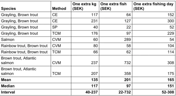
The final result for the Recreational Fishing group was the following intervals in Swedish kronor (SEK) for mean willingness to pay per recreational fisherman and default value for game fish:
• One extra kg: 13-207. Default value: 78. • One extra fish: 7-358. Default value: 105. • One extra fishing day: 17-229. Default value: 94.
Equivalent intervals and default values for other fish were as follows: • One extra kg: 5-79. Default value: 23.
• One extra fish: 2-16. Default value: 9.
• One extra fishing day: 7-158. Default value: 55.
It is proposed as a guideline for the use of these default values that the values are used by Swedish authorities in economic analysis relating to recreational fishing, provided the economic analysis does not concern a particular type of fish or fishing for which more specific values of satisfactory quality are available. Such specific values may, for example, be estimates of willingness to pay for a better angling or a particular species in a particular part of Sweden. When using the default values it should be borne in mind that they only capture the willingness to pay of
recreational fishermen. Non-recreational fishermen in all likelihood also have a considerable willingness to pay for improved recreational fishing.
The final result for the Water Quality group was the following intervals in SEK for mean willingness to pay and default values for reduced loadings of nitrogen and phosphorus to the coast:
• Nitrogen: 4-70 per reduced kg. Default value: 31.
• Phosphorus: 127-2140 per reduced kg. Default value: 1023.
Equivalent corrected intervals and default values for improvement in water clarity (measured as Secchi depth) in coastal waters of one metre were as follows:
• Per person and year: 268-369. Default value: 315. • Per visit: 45-360. Default value: 130.
It is proposed as a guideline for the use of these default values that the values are used by Swedish authorities in economic analysis relating to water quality, provided that the economic analysis does not concern a particular type of water quality for which more specific values of satisfactory quality are available. Such specific values may, for example, be estimates of willingness to pay for specific changes in water quality in particular water areas. In addition, the following circumstances should be considered when using the default values:
• They can be expected to be valid for improvements of quality in marine waters.
• It should be examined for each application relating to the default values for reduction of nitrogen or phosphorus whether it is reasonable to interpret a significant decrease in the nutrients as a halving.
• It should be borne in mind for each application relating to the default values for reduction of nitrogen and phosphorus that they are valid for extreme cases where either nitrogen loadings or phosphorus loadings have been halved. They thus cannot be used additively, for example for a valuation of 4000 kg less nitrogen and 40 kg less phosphorus.
• It should be examined for each application relating to the default values for improvements in water clarity whether it relates to a relationship between population and site of improvements which is comparable with the studies on which the default values are based.
In addition to the results above relating to intervals and default values, it can be noted that too few valuation studies exist in Sweden today to enable the existing need to value environmental change and impacts on ecosystem services to be satisfied. It would therefore be desirable to conduct a number of valuation studies on a broad front to enable more intervals and default values to be created and the intervals and default values calculated in this project to be updated. With a larger base of valuation studies it would additionally be possible to calculate intervals and default values by more advanced methods (e.g. quantitative analysis) than has been possible in this project. There is also a need for a clearly specified and uniformly valued change in the valuation studies carried out..
1 Introduction
1.1 Purpose of the project
The background to the project “Default values for environmental change and ecosystem services” is the need for and difficulties in describing changes to ecosystem services and the environment in monetary terms. This means that there is a great risk of environmental change and impacts on ecosystem services not valued in a satisfactory manner in economic analyses, for example in impact assessments and cost-benefit analyses. The purpose of the project is to draw up proposals for monetary default values for environmental change and ecosystem services with associated guidelines on how these values are to be applied. Using these default values, the Swedish authorities are to be able to make overarching and comparable descriptions of changes in ecosystems and the environment that follow from measures to achieve the environmental objectives. Jointly developed default values create the necessary basis for the Swedish authorities to describe changes of the environment and ecosystems in a uniform way. The project is in this way reminiscent of the ASEK work of the transport authorities, but is intended to lead to default values of a selection of environmental changes not covered by ASEK.1 The default values are not to be regarded as permanent but should be updated as new information becomes available, for example new results from new valuation studies.
The project is not a research project, and if the default values are to be well accepted among the users it is probably important that they are projected in a transparent and relatively non-technical way. Some authorities have pointed out in particular that it must be easy to see the link between the default values and the valuation studies on which the default values are based. At the same time, the results of the project must rest on a good scientific foundation. In addition, the project has been founded on a judgement that the default values should be based on valuation studies that reflect preferences among the population in Sweden. This can be justified by the default values being intended to be used by Swedish authorities in their economic analyses. In order to be able to assess how reasonable the default values produced are, however, it may be important to compare them with valuation results from other countries.
1.2 Arrangement of the project
The work under the project has been divided into the following three phases:2 1. Surveying (a) existing Swedish valuation studies, (b) what values are used
at present by Swedish authorities and (c) how any default values adopted should be designed to be usable in practice. The survey was conducted firstly by sending a questionnaire to a selection of Swedish authorities and secondly by reviewing existing Swedish valuation studies.
1 ASEK stands for Working Group for Valuation of Social Costs and Benefits of Transportations
(Arbetsgruppen för Samhällsekonomiska Kalkylvärden), see SIKA (2008).
2 The project has also come to include some updating of the valuation study database ValueBaseSWE
2. On the basis of results obtained in Phase 1 assessing for what environmental changes there is sufficiently detailed information on monetary values to enable them to be suitable for the development of default values, and creating intervals of monetary values for this selection of environmental changes.
3. On the basis of the intervals in Phase 2 assessing monetary value which could be used as a default value for the selected environmental changes.
1.3 Arrangement of the report
This report has been arranged as follows. Chapter 2 presents results from the survey in Phase 1, Chapter 3 discusses the selection of environmental changes and methodological issues which have been important in the development of intervals and how we have proceeded in dealing with these. Chapters 4 and 5 present a step-by-step practical description of how intervals have been created for valued changes in the groups of recreational fishing and water quality studies. These chapters also contain proposals for default values. We have also found several valuation studies which have valued conservation and other recreation (recreation excluding
recreational fishing). It has not been possible to create intervals for these groups, as described in Chapter 6. The report ends with an attempt to compare the project’s default values internationally and a concluding discussion in Chapter 7. Three appendices and two annexes are also attached to the report.
The report assumes that the reader has some prior understanding of economic valuation of the environment and how such values can be used in economic analyses. Introductions to these topics are presented for example in previous reports from the Swedish Environmental Protection Agency (e.g. 2003, 2004a, 2004b, 2005), in ASEK reports (e.g. SIKA, 2008) and in more general literature such as Brännlund and Kriström (1998), Hultkrantz and Nilsson (2008), Mattsson (2006) and Söderqvist et al. (2004).
2 Surveying of monetary values
This chapter presents the results of the first phase of the project, i.e. the surveying of (a) existing Swedish valuation studies, (b) what values are used at present by Swedish authorities and (c) how any default values adopted should be designed to be usable in practice. The survey concerning (a) was primarily done using existing databases of valuation studies, see section 2.1 below. (b) and (c) were surveyed using a questionnaire sent to the nine key environmental objectives authorities (National Board of Housing, Building and Planning, Swedish Board of Agriculture, Swedish Chemicals Agency, Swedish Environmental Protection Agency, National Heritage Board, Swedish Forest Agency, National Board of Health and Welfare, Swedish Radiation Safety Authority and Geological Survey of Sweden) as well as a selection of other Swedish authorities for which environmental valuation can be expected to be a particularly relevant area: the National Rail Administration, the Swedish Board of Fisheries, the National Institute of Public Health, the National Institute of Economic Research, Luftfartsverket (the national airports authority), the Swedish Institute for Transport and Communications Analysis (SIKA), the National Maritime Administration, the Swedish Transport Agency, the Water Authorities and the National Road Administration. The questionnaire results are summarised in Section 2.2.
2.1 Compilation of Swedish valuation studies
To review Swedish valuation studies an inventory was made of studies in the Swedish valuation study database (ValueBaseSWE), the Nordic valuation study database (NEVD) and the global valuation study database (EVRI).3 The inventory focused on Swedish primary studies, i.e. studies based on Swedish primary data, and a total of 141 studies were found. A general list of these studies is presented in Appendix 1. Detailed information concerning these studies can be found in the separate file Översikt.xls.4 As ValueBaseSWE and NEVD are not regularly updated at all and EVRI is only updated slowly, most of the valuation studies done in the past few years are not included in the table. In addition, around 15 studies are not included because they are difficult to classify – they may have valued such
different things as blood pressure and pork production. Background reports or parts of theses which are covered by other documents and are therefore “duplicates” are not included. Studies covered by ASEK are as far as possible sifted out, as they have already been used as material in ASEK work. The general usability of the ASEK values of costs and benefits has been the object of special analysis during the course of the project, see also Section 3.1.
3 ValueBaseSWE: Valuation Study Database for Environmental Change in Sweden
(www.beijer.kva.se/valuebase.htm).
NEVD: Nordic Environmental Valuation Database (www.norden.org/pub/sk/showpub.asp?pubnr=2007:518)
EVRI: Environmental Valuation Reference Inventory (www.evri.ca).
4 Översikt.xls and a number of other files (see next section) are included as background material to this
Just over 20 per cent of the 141 collated studies are national, i.e. the sample in the study represents the national Swedish population. The year stated in the “Year” column in Appendix 1 relates to the year of data for the study concerned, and this also applies to Figure 1 below. Around 30 of the total number of studies were done in the 1980s, around 70 in the 1990s and around 30 in the 2000s, see Figure 1 below.
Figure 1. The year of data for the 141 collated studies
The studies were classified into groups on the basis of the object of valuation. The starting point for this grouping was the data categories “Asset - general
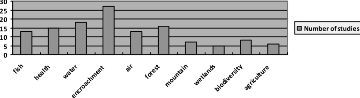
environmental asset” and “EGS - general type of environmental goods and services valued” in EVRI and NEVD and “Environmental goods/services” and “Extent of environmental change” in ValueBaseSWE. It can be difficult to judge in which group to classify a study, and some studies are therefore included in the table several times if they match more than one group. In the “Valued change” column in Appendix 1 the studies in each group are roughly classified according to what change has been valued in the study. Figure 2 below shows how the studies are classified across these groups. Note that only groups containing at least five studies are included in the figure. The groups containing fewer than five studies are “foods”, “ecosystem services”, “aircraft-related noise” and “radiation environment”.
Figure 2. Classification of the studies on the basis of the object of valuation
0 10 20 30 40 50 60 70 80 1980s 1990s 2000s Number of studies 0 5 10 15 20 25 30 fish heal th water encr oach men t air fore st mount ain wetla nds biod iver sity agric ultur e Number of studies
Among the collated studies, the greatest number of valuation studies concern encroachment impacts, while many studies concern transport and traffic and various infrastructural changes in society. These subject areas are also addressed in some of the valuation studies concerned with air quality. Studies concerned with lakes, seas and other aquatic environments as well as fishing are also common among the collated valuation studies.
The valuation method used varies between the collated studies. A list follows below of the abbreviations used in the “Valuation method” column in Appendix 1. In addition, WTP will also be used as the abbreviation for willingness to pay. Revealed preference (RP) methods :
DE Defensive expenditure method HP Hedonic price method
PF Production function method TCM Travel cost method
Stated preference (SP) methods:
CE Choice experiments
CVM Contingent valuation method
Other valuation methods:
HCM Human capital method pWTP Political willingness to pay
RC Replacement costs
REC Restoration costs
CVM is by far the most widely used method among the collated studies. Next comes CE (including “conjoint analysis”, which is usually another name for CE) and TCM, see Figure 3 below. Other valuation methods are evenly distributed among the remaining studies and have been used relatively little. It can be added that RP and SP methods are firmly entrenched in economic theory, while the group of “other valuation methods” contains methods which are not as solidly rooted in common economic theory and may therefore provide results that are difficult to interpret, see for example Swedish Environmental Protection Agency (2005).
Figure 3. Distribution of studies on the basis of method of valuation
To summarise, a relatively small proportion of the collated valuation studies have been done with a national population selection. Most of them were done in the 1990s, but this may change as databases are updated and studies from the 2000s are
0 20 40 60 80 100 CE CVM Conj oint anal ysis DE TCM SP REC RC PF HP Politi cal W TP Valuation method
included. A large proportion of the collated valuation studies concern
environmental change linked to infrastructure investments, while many are also concerned with fish and the aquatic environment. CVM is the most common valuation method.
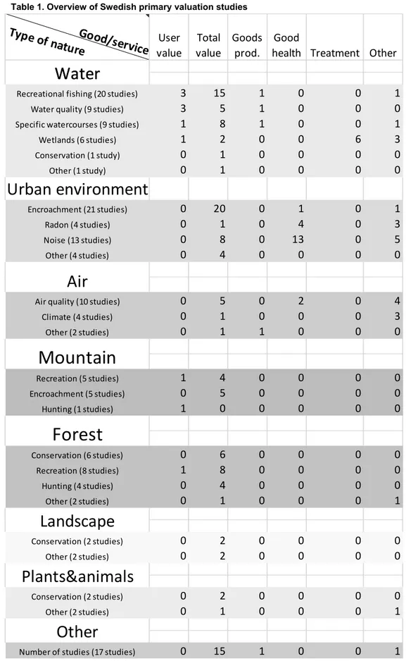
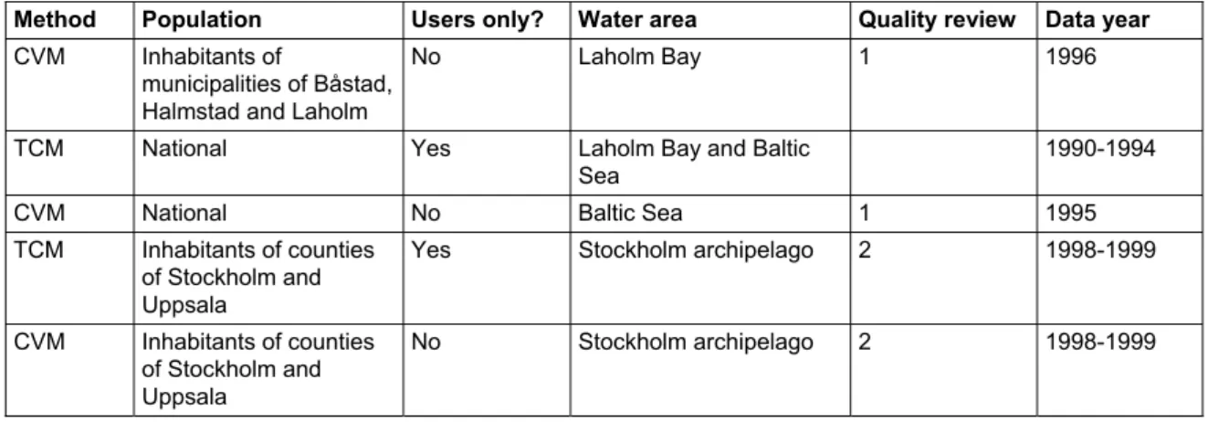
Table 1 shows the valuation studies in Appendix 1 and Översikt.xls in the form of a cross-table from which it is possible to read off the number of studies which have valued a particular “type of nature” and a particular good or service. The intention with this cross-table is to indicate for which selection of “types of nature” it is potentially possible to create intervals for monetary values and default values and what goods/services have been valued in these studies. Note that columns must not be added together with other columns (the same applies to rows) as one study may appear in more than one place. We will return to this selection in Chapter 3.
Table 1. Overview of Swedish primary valuation studies
Good/se
rvice
Type of n
ature
Uservalue Total value Goods prod. Good
health Treatment Other
Water
Recreational fishing (20 studies) 3 15 1 0 0 1
Water quality (9 studies) 3 5 1 0 0 0
Specific watercourses (9 studies) 1 8 1 0 0 1
Wetlands (6 studies) 1 2 0 0 6 3 Conservation (1 study) 0 1 0 0 0 0 Other (1 study) 0 1 0 0 0 0
Urban environment
Encroachment (21 studies) 0 20 0 1 0 1 Radon (4 studies) 0 1 0 4 0 3 Noise (13 studies) 0 8 0 13 0 5 Other (4 studies) 0 4 0 0 0 0Air quality (10 studies) 0 5 0 2 0 4
Climate (4 studies) 0 1 0 0 0 3 Other (2 studies) 0 1 1 0 0 0 Recreation (5 studies) 1 4 0 0 0 0 Encroachment (5 studies) 0 5 0 0 0 0 Hunting (1 studies) 1 0 0 0 0 0 Conservation (6 studies) 0 6 0 0 0 0 Recreation (8 studies) 1 8 0 0 0 0 Hunting (4 studies) 0 4 0 0 0 0 Other (2 studies) 0 1 0 0 0 1 Conservation (2 studies) 0 2 0 0 0 0 Other (2 studies) 0 2 0 0 0 0 Conservation (2 studies) 0 2 0 0 0 0 Other (2 studies) 0 1 0 0 0 1
Number of studies (17 studies) 0 15 1 0 0 1
Other
Water
Air
Mountain
Forest
Landscape
Plants&animals
2.2 Collation of questionnaire responses from
authorities
The questionnaire entitled “A questionnaire to survey authorities’ use of and need for monetary values to describe environmental change and impacts on ecosystem services” was sent at the beginning of March 2009 to the following authorities: The National Board of Housing, Building and Planning, the Swedish Chemicals
Agency, the Swedish Environmental Protection Agency, the National Heritage Board, the Swedish Forest Agency, the National Board of Health and Welfare, the Swedish Radiation Safety Authority and the Geological Survey of Sweden, the National Rail Administration, the Swedish Board of Fisheries, the National
Institute of Public Health, the National Institute of Economic Research, the airports authority Luftfartsverket, SIKA, the National Maritime Administration, the
Swedish Transport Agency, the Water Authorities and the National Road Administration.
The purpose of the questionnaire was to survey the current use of and need for default monetary values to describe environmental change and impacts on ecosystem services. The survey, with the collated responses from the authorities, can be found in its entirety in Appendix 3. A briefer summing-up of the responses follows below.
In Question 2 the authorities were asked whether they use default monetary values to describe environmental change and impacts on ecosystem services. The majority of the responding authorities use such values. There appears, however, to be a need for and a lack of such values but also doubt and uncertainty over what values are to be used and how. The values are used in impact assessments, among other uses. Some authorities do not use these monetary values as they endeavour to achieve cost-effectiveness for a specific objective.
Question 3 of the questionnaire was concerned with documents in which the authorities use default monetary values to describe environmental change and impacts on ecosystem services. Many of the documents mentioned here are linked to inquiries and reports produced as part of the work of the authorities on the environmental objectives. Monetary values have also been used by the authorities in economic analyses and calculations and in the authorities’ own inquiries. In Question 4 the authorities were asked to list the environmental changes/impacts on ecosystem services for which the authorities use monetary values and what values are used for these. They were also asked to explain how the values were produced or to indicate a source reference. Many of the environmental
changes/impacts on ecosystem services described by the authorities in monetary terms related to conservation of various natural assets, increased populations of various species and biodiversity. Most of the authorities also used monetary values for air pollutants and emissions of nitrogen and phosphorus. The values used by the authorities were stated in SEK/kg but also in SEK/licence, SEK/household and other units. Some environmental changes/impacts on ecosystem services were also
valued in terms of loss of production, costs of measures or damage costs. The values principally come from valuation studies, the authorities’ own inquiries, SIKA or IVL.
Under Question 5 the authorities were asked to indicate documents or reports describing how the authority uses monetary values to describe environmental changes/impacts on ecosystem services. There were lacking at many authorities, while several referred to the ASEK4 report (SIKA, 2008).
In Question 6 the authorities were given an opportunity to indicate for what environmental change/impacts on ecosystem services they need/use default monetary values and in what unit they would prefer to see these expressed. A conclusion based on this question is that the default monetary values the authorities are looking for are closely linked to the work of each authority, which means few overlaps. It is therefore difficult to draw general conclusions on the values for which there is a particularly great need. There appears, however, to be a great need for default monetary values for emissions of different chemical substances, heavy metals, oil, nitrogen oxide, sulphur oxide, carbon dioxide, nitrogen and
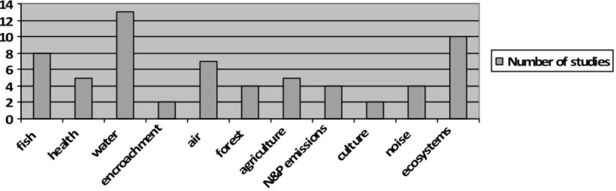
phosphorus. Examples of units the authorities would like to see for these are SEK/kg, SEK/dispersed quantity, SEK/ha or SEK/m3. There is also a need for default monetary values for impacts on ecosystems, watercourses, fish, wetlands, extraction of natural resources such as stone, gravel and water and conservation of natural resources. The changes for which the authorities would like to see default values are divided into groups in Figure 4, as in Figure 2 above. The classification is rough and was made for those groups in which there were at least two changes for which there was no monetary value. Mountains, wetland and biodiversity are therefore not included as groups in the diagram below. On the other hand there are wishes for default monetary values for different phosphorus and nitrogen
emissions, impacts on different ecosystems, noise and impacts on cultural environments.
Figure 4. Authorities’ wishes regarding default values
In question 7 the authorities had to indicate what would be needed at the authority to make it easier to use monetary values to describe environmental change and impacts on ecosystem services. Many authorities indicated here that there is a need
0 2 4 6 8 10 12 14 fish health wat er encr oach men t air fore st agricu lture N&P emissi ons cultu re noise ecos ystem s Number of studies
for more research and additional studies to create more data in the area. Repeated studies on the same environmental change to reduce uncertainty were welcomed. Better coordination between authorities, acceptance of default monetary values, uniform, comparable indicators and expertise in environmental economics were also looked for.
Finally the responding authorities were given an opportunity to present other comments and opinions under Question 8. Some authorities stated that the questionnaire was difficult. It was also stated that it would be desirable to have clearly defined terms, fundamental guidelines for the work and recommendations for the development of units and for authorities to value the same type of change in a uniform manner. It was also mentioned that projects like this are important, that there is a lack of studies in the area, that many biological correlations are unknown, which poses problems, and that results obtained are difficult to generalise.
3. Method for development of
intervals and default values
3.1 Selection of environmental changes
To enable meaningful intervals of monetary values and default values to be created, it is firstly necessary for there to be a sufficient number of studies whose results can be used as observations to create a interval. It is difficult to define in advance what a “sufficient number” is. It is sufficient in principle to have two observations, but there is likely to be a risk of such a interval not being robust. Secondly the studies that make up the observations are required to be relatively homogeneous with regard to what has been the object of valuation. There is otherwise a great risk of the results of the studies not being mutually comparable. It is judged on the basis of the need for a sufficient number of relatively
homogeneous studies, the information in Table 1 and our knowledge of the studies included in Table 1 that meaningful intervals can potentially be created for the following groups:
1. Recreational fishing 2. Water quality 3. Conservation
4. Other recreation (recreation excluding recreational fishing) Following discussions with the reference group it was additionally judged
reasonable for the work on intervals to follow the order of priority indicated in the list above. It has been possible to create intervals of monetary values for the groups of Recreational Fishing and Water Quality. These intervals are presented in
Chapters 4 and 5 respectively. The groups of Conservation and Recreation excluding Recreational Fishing have been judged to be too heterogeneous in the change valued in each study for it to be possible to create intervals for these groups, as explained more fully in Chapter 6.
It can be seen from Table 1 that there are relatively many studies in groups under Urban and Air. Default values for these environmental changes have to some extent already been calculated in the context of ASEK work. Gunnel Bångman at SIKA has therefore made a special investigation during the course of the project of whether ASEK values relating to the following areas are suitable for use as general default values outside the transport sector: (a) loss of life and health as a
consequence of road-traffic accidents, (b) air pollutants from burning of fossil fuels and (c) noise. A report on this can be found at Annex A. To summarise, this report notes the following (see Annex A for details):
a. The ASEK value of a statistical life (VSL) for road-traffic accidents should be usable as a general valuation of life and health.5
b. The ASEK value for carbon dioxide emissions should not be used outside the transport sector.
c. Some of the ASEK values for local and regional impacts of air pollution may be usable as general default values, others not.
d. The ASEK value for noise should not be used as a general default value.
3.2 Methodological issues
To enable usable intervals to be created for valued environmental changes it is of key importance that the values within the interval are mutually comparable. Account needs to be taken of a number of different aspects to create comparability. In sections 3.2.2 and 3.2.3 above we examine how we have in general dealt with the following two aspects:
1. Expressing the environmental change which has been the object of valuation in the same physical unit.
2. Expressing the estimated economic value in the same monetary unit. The more detailed procedure we have followed in creating comparability for the cases of Recreational Fishing and Water Quality is described in Chapters 4 and 5. Before we examine these two aspects, we resent an account in Section 3.2.1 of how the intervals in principle will be designed and how a default value can be identified on the basis of the observations underlying the intervals.
3.2.1 Design of intervals and calculation of default values
It should first be clarified what we mean by “observation” in this context. We will be concerned with various valuation studies that have estimated the economic value of a particular economic change. We regard such an estimate as an
observation if it is based on particular data material. The observation is typically equal to the main estimate of the economic value presented in the valuation study. A single valuation study may, however, lead to more than one observation if it presents more than one estimate because it has made use of more than one set of data, for example several different questionnaires. It is, however, common for a valuation study to present several different estimates not because several different sets of data have been used but because different estimation methods have been used on the same set of data. In such a case the study only, however, leads to one observation, which is identical to the estimate which the study presents as the principal estimate or, if it is not explicitly apparent from the study which is the principal estimate, identical to the mean value of the estimates presented in the study.
However, only in exceptional cases is it directly possible to pick estimates from individual valuation studies to obtain observations for the interval. As indicated above, although the environmental changes have been grouped in a way that gives reason to believe that there is fundamental comparability between the results of the
different valuation studies, it will be necessary to make various conversions of the basic results of the studies to obtain such great comparability that they can
represent observations for the interval. As explained in more detail in Chapter 4, some recreational fishing studies, for example, have estimated the economic value of catching one extra fish and others have estimated the value of catching one extra kg of fish. It is desirable to be able to convert one value to the other so that
observations are not lost.
Assume, by way of example, that we are concerned with three recreational fishing studies, A, B and C, of which A and B have estimated mean willingness to pay to obtain one extra kg of fish for SEK 10 or 15, i.e. WTPA = SEK 10/kg and WTPB = SEK 15/kg. Study C, on the other hand, has estimated the mean willingness to pay for one extra fish at SEK 25, i.e. WTPC = SEK 25/fish. If a fish on average weighs 0.5 kg, WTPC can be converted to a mean willingness to pay to obtain one extra kg of fish by dividing by the mean weight: 25/0.5 = SEK 50. A interval for mean willingness to pay per kg fish can be formed from these three observations extending from the minimum value of SEK 10 to the maximum value of SEK 50, i.e. SEK 10-50.
The interpretation of this interval is that it indicates that if we wish to say
something about the mean willingness to pay per kg fish for an arbitrarily chosen improvement in recreational fishing, this mean willingness to pay is somewhere within the endpoints of the interval. This interval is broad in the sense that it does not give any distribution of probability for the values within the interval, but it can be interpreted as only providing the information that the probability of the
willingness to pay being in the interval SEK 10-50/kg is equal to 1 and that the probability of the willingness to pay being outside the interval SEK 10-50/kg is equal to 0. However, it is likely that there is some kind of distribution of probability for the values within the interval. It may be a uniform probability distribution, but the three observations in the example – 10, 15 and 50 – perhaps indicate that it is more likely that the mean willingness to pay for an arbitrarily chosen improvement is somewhere in the lower half of the interval than in its upper half. Saying something on the basis of the observations that constitute the
endpoints of the interval and the observations which are within the interval about what value of mean willingness to pay per kg fish for an arbitrarily chosen improvement is the most likely one, is what we regard as a way of creating a default value.
There are various ways of proceeding to estimate what value is most likely, for example resampling (“bootstrapping”). A quantitative meta-analysis of the observations is another option, which additionally could provide information on how characteristics of the studies which have led to the observations affect the magnitude of the estimated economic values. It will, however, be apparent from Chapters 4 and 5 that the intervals which it has been possible to construct are based on a small number of observations – fewer than 10. We have therefore judged it not to be reasonable to use special quantitative techniques to create default values and will instead regard the default value as equal to the mean value of the observations
on which the intervals have been based.6 The default value for the above example would therefore be (10+15+50)/3 = 25. Each observation will be weighted equally in the calculation of the default value. The reasonableness of this can be
questioned, as the studies from which the observations originate may differ for example with respect to the time when they were performed and their quality. We shall return to these aspects in Section 3.2.3 below.
Finally it should be noted that the interval SEK 10-50 is narrow in the sense that it is constructed on the basis of point estimates of mean willingness to pay and the mean weight of the fish. An alternative would have been to create the interval using the endpoints of the confidence interval7 for mean willingness to pay and the mean weight of the fish. Assume, for example, the following confidence intervals for WTPA, WTPB, WTPC and the mean weight: SEK 5-15/kg, SEK 8-22/kg, SEK 15-35/fish and 0.4-0.6 kg/fish. This, taken together, would produce the interval SEK 5-87.50/kg, i.e. a significantly wider interval than SEK 10-508. We form intervals below on the basis of point estimates of mean values, and it is important to remember that this contributes to making the intervals relatively narrow. 3.2.2 Uniform physical units
The above example of three recreational fishing studies which have valued improved recreational fishing but have used different indicators of improved recreational fishing illustrates the importance of being able to express the actual environmental change in the same physical unit. This contributes to creating comparability between the studies and increasing the number of observations. As indicated in Chapter 4, many recreational fishing studies have examined the value of improved recreational fishing opportunities in terms of increased catch in number of fish or number of kg or an increased number of fishing occasions/days. We have judged it possible for these studies to make conversions between the three ways of measuring improved recreational fishing authorities, so that the
improvement is measured in three ways for all studies. The procedure is described in detail in Chapter 4.
For the second case studied in this report – water quality – we note that the studies concern the impact of eutrophication on water quality. It is therefore natural to link the studied environmental change to changes in loadings of the nutrients nitrogen and phosphorus, measured in kg per year. This is done in Chapter 5. In this chapter use is also made, however, of the fact that several of the studies have quantified the change in quality as a changed water clarity. This made it possible to also use water clarity (in metres) as a uniform physical unit.
6 The observations may, however, be usable for future meta-analyses if they can be supplemented by
results from more valuation studies.
7 The confidence interval is a measure of the uncertainty that exists when we attempt to estimate a
mean value.
3.2.3 Uniform monetary units
3.2.3.1 WELFARE MEASURES
In the rich flora of valuation methods there are such that are aimed at estimating changes in consumer surplus and those which are aimed at changes in producer surplus9. Studies that have used the former type of valuation methods dominate in number, and we have focused on them to obtain as good uniformity as possible. These studies vary, however, with regard to which monetary measure or measures have been estimated, e.g. mean willingness to pay, median willingness to pay or (the mean value of) the marginal willingness to pay, see also below. They may also differ with regard to what type of change in consumer surplus – compensating variation, equivalent variation or changes in Marshallian consumer surplus – the studies have intended to estimate.10 We have not, however, differentiated the studies according to this difference.
With regard to mean willingness to pay or median willingness to pay we have consistently chosen to make use of estimates of mean willingness to pay. This is a natural choice in view of the fact that the whole project is intended to provide information that can be used as a basis for cost-benefit analyses and socio-economic impact analysis. It is sufficient in such analyses to have information on the total willingness to pay for all individuals affected, which is estimated by multiplying the mean willingness to pay by the number of affected individuals. A mean willingness to pay of SEK 50/person for a population of 1 million
individuals, for example, gives a total willingness to pay of SEK 50m. Median willingness to pay cannot be used in the same way to calculate a total willingness to pay. In view of the sensitivity of mean willingness to pay to (high) outliers it has, however, sometimes been suggested that it is reasonable to make use of median willingness to pay as a cautious estimate of mean willingness to pay. We have, however, retained mean willingness to pay as valuation studies usually sift out outliers judged to be unrealistically high.
We have, furthermore, consistently assumed that the valued environmental changes are characterised by constant marginal utility and have therefore been able to equate mean willingness to pay spread per physical unit with marginal willingness to pay. This assumption means among other things that in principle we do not make any distinction between cases characterised by different baseline situations with regard to the valued environmental improvement. This is a strong assumption, as it is more reasonable to imagine a declining marginal utility, i.e. the value of a unit of better environmental quality being higher if the environmental quality in the baseline situation is relatively low than if the environmental quality in the baseline situation is relatively high. The assumption of constant marginal utility makes a strong contribution to creating comparability between the studies, but at the price
9 Changes in consumer and producer surplus are a measure of a change in wellbeing for consumers
(individuals and households) and producers (firms). Households/individuals and firms are the two most important market actors studied in microeconomics and are therefore also important in this applied analysis.
10 Compensating variation, equivalent variation and changes in Marshallian consumer surplus are
of introducing a fairly unrealistic assumption. It would be desirable to soften the assumption of constant marginal utility, for example by attempting to make a distinction between studies based on substantially different baseline situations regarding the valued environmental quality. It has not, however, been possible to do so in the framework of the present project.
3.2.3.2 METHOD-SPECIFIC CORRECTIONS
Valuation methods aimed at measuring willingness to pay are usually divided into stated preference methods (SP methods) and revealed preference methods (RP methods). The former are controversial, partly because they are based on individuals’ response to a hypothetical market situation in the framework of an interview or questionnaire-based study. There are strong indications that there is hypothetical bias, i.e. a distortion due to individuals’ action in a hypothetical market differing from the action which would occur if the hypothetical market situation became reality. This would mean that the willingness to pay estimated by SP methods is significantly different than the “actual” willingness to pay. Estimates based on SP methods are not likely to find broad acceptance until it can be credibly claimed that there is no hypothetical bias or that this is at least insignificant. Mikael Svensson at Örebro University has therefore conducted a special review of the scientific literature concerning this hypothetical bias, see Annex B. His review shows clearly that SP studies tend to produce a substantial hypothetical bias if the studies have not made use of special methods to reduce this bias. To correct the mean willingness to pay from SP studies for the occurrence of hypothetical bias a calibration is proposed in which mean willingness to pay is divided by three. This is not to be interpreted as meaning that the hypothetical bias for each individual SP study amounts to a factor of 3. On the contrary, the magnitude of the bias is likely to depend on many factors in addition to special methods for reducing hypothetical bias, for example what environmental change has been the object of valuation and what type of question has been asked in the SP study to obtain information on the respondents’ willingness to pay. There is no detailed knowledge at present,
however, on how such aspects affect the magnitude of the hypothetical bias. In our work with intervals and default values we have therefore consistently applied the correction factor 3, but in order to make this correction as transparent as possible we present intervals and default values in Chapters 4 and 5, firstly before
correction for hypothetical bias and secondly after this correction.11
Correcting responses to questions on willingness to pay afterwards is somewhat controversial. If the correction procedure becomes generally known, will future respondents in SP studies not take account of this when giving their responses to the questions on willingness to pay, for example by multiplying their willingness to pay by 3? If so, a correction factor will evidently only be valid during a limited time, which would lead to increased confusion concerning the degree of hypothetical bias. The trend is, however, towards SP studies with increasing regularity making use of special methods to reduce hypothetical bias. We therefore
11 A different correction factor is probably suitable for SP studies which have examined compensation
requirements instead of willingness to pay. The SP studies used for the intervals in this study have all, however, studied willingness to pay.
regard the correction for hypothetical bias as almost a one-off measure to deal with previous studies which have not made use of such special methods. The risk of the correction influencing the responses of future respondents ought therefore to be small.
Another fundamental difference between SP methods and RP methods is that the SP methods, unlike RP methods, can capture the willingness to pay of non-users for environmental improvements. We have not made any correction for this reason, but it should be noted that this difference may potentially explain why a interval becomes wide. All other things being equal, a wide interval can be expected to arise if the interval is formed from observations from both RP studies and SP studies of an environmental improvement for which there are high non-user values. It should be noted that there are many other corrections it is potentially reasonable to make. Attention has, for example, been drawn to the fact that for SP studies estimates of mean willingness to pay may be sensitive to what assumption is used with regard to the statistical distribution of willingness to pay, for example whether the willingness to pay is assumed to be greater than zero or whether a willingness to pay equal to or less than zero is also possible. We have, however, consistently assumed that the authors of the valuation studies have based their estimations of mean willingness to pay on reasonable assumptions. Where it is not obvious which estimate of mean willingness to pay is the principal estimate of the study, however, we have calculated a mean value of the estimates presented in the study, cf. Section 3.2.1.
Both SP studies and RP studies are often based on questionnaire studies of a random sample of a particular population. Some level of non-response is
unavoidable, and studies differ with regard to how non-respondents have been dealt with. In some studies the group of non-respondents has been assumed to have a willingness to pay equal to zero and in this way is counted in the estimate of a mean willingness to pay for the whole population. Other studies have only calculated mean willingness to pay based on the respondents’ responses and in calculating the mean willingness of the population to pay have implicitly assumed that the group of non-respondents has a mean willingness to pay as high as that of the group of respondents. We have not systematically studied how the group of non-respondents has been treated in different studies with the aim of correcting for any differences, and have instead assumed that the studies’ authors have made a reasonable assessment in handling the group of non-respondents. We note, however, there is often reason for valuation studies to contain a deeper non-response analysis than is usually done, as estimates of the magnitude of the mean willingness to pay of the population may be greatly influenced by different
assumptions on the mean willingness to pay of the non-respondents, particularly as the group of non-respondents is large in some studies (over 50% of the sample). 3.2.3.3 TIME CORRECTIONS
Corrections for changes in price and income levels are required for the monetary values to be comparable. To achieve this, they have been calculated so that they are valid for a particular year. In our case we have chosen 2006, as this is the base-year
for the estimates in ASEK4. We also follow the same conversion procedure as in ASEK4, i.e. (1) adjusting for inflation by using the consumer price index (CPI) to convert values to a uniform price level and (2) adjusting estimates of willingness to pay for increases in income over time by using an index for real GDP per capita (SIKA 2008, p 63-67). Values not based on estimates of willingness to pay, however, only have to be adjusted for inflation.
Using an index for GDP per capita to adjust estimates of willingness to pay signifies an assumption that the income elasticity of willingness to pay is equal to 1. SIKA (2008) justifies this by referring to certain research results. The
assumption can, however, be questioned as other research results suggest that the income elasticity of willingness to pay for environmental change in Sweden tends to be lower than 1 (Hökby and Söderqvist, 2003). These results are, however, based on cross-sectional data, and it is not obvious what they signify for the trend in willingness to pay from a time-series point of view. There is therefore reason for the time being to retain the method of using real GDP per capita. It would
nevertheless be desirable for the method to be evaluated in coordination with the ASEK work.
It should be emphasised that the above correction does not take account of the fact that people’s preferences may change over time. Increased attention on and/or knowledge of an environmental issue may, however, be expected to lead to a change in people’s willingness to pay, either temporarily or permanently. Change of preferences may also be a generational issue. It would therefore be advantageous in calculating a default value for it to be possible to assess to what extent each observation in the interval is outdated on the basis of a preference perspective and to let this assessment form the basis of a weighting procedure. We have not, however, found it possible to make such an assessment which is not arbitrary and have therefore refrained from adopting a weighting procedure. There is a need for identically arranged valuation studies to be performed at different times to enable reliable knowledge to be obtained on such changes. Another factor is that the vast majority of the studies in Chapters 4 and 5 are used to create intervals which have been implemented within a 10-year period. It is thus at least not a matter of observations concerning entirely different generations of people.
3.2.4 Other general considerations
It ought to be apparent from the preceding section that it has often been necessary to make a large number of conversions of the basic estimates in the valuation studies to obtain a usable observation for the intervals. In addition, the conversions in some cases are based on broad assumptions. To make it possible to understand the calculations, and adjust them with relative ease if new information becomes available in the future, we have chosen in Chapters 4 and 5 to present our procedure step by step. All the conversions and the assumptions on which these rest are explicitly apparent from the separate Excel files listed in Appendix 2. Finally it can be pointed out that designing and carrying out a valuation study is no easy task and is often demanding on resources. Different valuation studies can
therefore be expected to be of variable quality. Forty of the studies included in Table 1 have been the object of quality review (Soutukorva and Söderqvist, 2006) on the basis of the Swedish Environmental Protection Agency’s quality criteria for environmental valuation studies (Swedish EPA, 2005; Söderqvist and Soutukorva, 2009). Prior to the creation of intervals, a check was made that no study was included which in the quality review was found to have deficiencies making it unsuitable for use in policy contexts.12 It would be desirable for all studies which form intervals to have been subject to quality review on the basis of the Swedish Environmental Protection Agency’s quality criteria, but it has not been possible to implement this under this project.
The information on quality which has been available provides information on whether a valuation study has passed a particular quality threshold, but not necessarily on which study is the best of all. If it had been possible to rank observations for a interval in terms of quality, the calculation of default values could have been based on a weighting procedure in which the best study of all is given the heaviest weighting of all or is simply given the weighting 1, i.e. the default values are entirely derived from this study. The problem is that the number of potential sources of error and uncertainties is so great that it is difficult for even very well produced and large studies to take account of everything. In an SP study, for example, the number of choices regarding the formulation of the willingness-to-pay questions and the components of the valuation scenario is so high that it is not possible to test everything in the context of a single study. This is an important reason why results from meta-studies tend to have great scientific weight, not just in the field of economics. Although this does not support the method of basing default values on individual studies, it would be desirable to let studies of relatively high quality weigh more heavily in the calculation of default values than studies of relatively low quality. We have not, however, been able to identify any reasonable method of making such a ranking, and all studies which have passed the quality threshold have been weighted equally heavily in the calculation of the default values. As mentioned above, however, some studies which have not been subject to quality review on the basis of the Swedish Environmental Protection Agency’s quality criteria are included. These have been assessed by us on an ad hoc basis as not being inferior from a quality point of view, but it would advantageous for future projects to make it possible for these studies also to be subject to quality review.
12 The basic grades in the quality review by Soutukorva and Söderqvist (2006) were: 1. “No serious
deficiencies were discovered”. 2. “A more detailed review should take place if the study is to be used in policy contexts.” 3. “The study has deficiencies making it unsuitable for use in policy contexts. Prior to the creation of intervals a check was made that no study graded 3 was included.
4 Intervals for recreational fishing
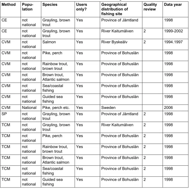
A description follows below of the procedure for creating intervals for the group of valuation studies of recreational fishing. The first step was to supplement the 18 recreational fishing studies collated from the three valuation study databases ValueBaseSWE, NEVD or EVRI with valuation studies not contained in the databases as they either were created after the first two databases were collated or are only in Swedish and are therefore not included in EVRI. It is desirable to include all Swedish studies in order to obtain a broad data material with as many observations as possible. The material has been principally supplemented by making contact with persons who are familiar with the valuation of recreational fishing and who were asked to list recreational fishing studies made in recent years. A total of 12 new studies were added, and the data material then consisted of 30 studies. Some of these studies were different versions of the same study, for example in report form, as a draft or in another edition. A published scientific article was preferred to other publications of the same study, and seven studies had to be removed for this reason. Another three studies were removed: the first proved not to be a valuation study (and therefore not to be relevant), while the other two were removed because they estimated changes in producer surplus and are therefore not relevant for use in the formation of intervals, see section 3.2.3.1 above. There finally remained 20 studies, of which three could not be obtained because they were not available through databases, the websites of university institutions or other electronic library resources. The final material consequently consists of 17 recreational fishing studies. Six of these 17 studies are national, and in 11 the population is fishermen (users). With regard to method, nine are CVM studies, four are CE studies and four are TCM studies. For detailed information about these studies, see the file “Detaljinformation fritidsfiskestudier.xls13” in Appendix 2.
4.1 Physical comparability
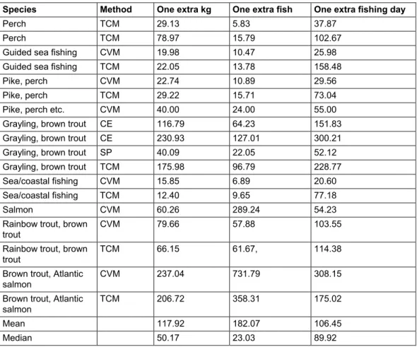
A large proportion of the work entailed expressing the environmental change which has been the object of valuation in the same physical unit and then as far as possible expressing the estimated economic value in the same monetary unit. With regard to the first type of fundamental conversion, intervals have been created for three different changes: obtaining one extra kg of catch, catching one extra fish and obtaining one extra fishing day. These changes were chosen as most of the
valuation studies in this group had valued one of them. Another reason for focusing on these changes is that if there is a correlation between the changes they can be mutually translated, and three values can then be created for each study. The studies included in the calculations of intervals are studies where there are estimates for one or more of these three changes. If a study for example has estimated the value of catching one extra fish, this value, through a conversion procedure, can be used to estimate the value of one extra kg of catch and one extra fishing day. The conversion procedure makes it possible to compare estimates in
studies which have valued different (but close) changes while at the same time broadening the data material. The common unit providing these correlations between different valued changes in the studies is weight.
Weight constitutes the common conversion unit and means that the species of fish studied in the study concerned becomes important as the species is one of the deciding factors for the weight of the fish. The species was specified in all the studies later used to create intervals except one. In this study (reference number14: T4), which is a national fishing study from 2006, all species caught in 2006 were indicated and the ten most caught species (with hand gear) were assumed to be the most important for the calculations of interval.
The species studied in the study concerned was thus specified in the vast majority of cases, but the weight of the studied species was not stated in the study to the same extent. In three of the studies (reference numbers A5, P5 and P6) used for interval calculations the weight for the studied species was not specified. The conversions were made for other studies using information on the mean weight for the species usually caught in recreational fishing. This information has been collated by Håkan Carlstrand at the Swedish Board of Fisheries following
discussions with his colleagues. Carlstrand emphasises the difficulty of making this type of general estimation as Sweden has a large number of watercourses and lakes and a very long coastline, these watercourses contain saltwater, freshwater and brackish water and the quality of both waters and fish stocks varies heavily. When species and weight for each study have been specified, the average weight for the studied species can be calculated. In three of the studies (reference numbers A5, S28 and S29) used for the interval calculations only one species has been studied. In the case of those studies which studied two or more species, a mean weight was calculated for the caught species, and the catch was assumed to be evenly distributed across the studied species.15 The average weight for the species studied is one of the units required to be able to translate estimates of “one extra fish” to “one extra kg” and vice-versa.
One extra day of fishing has been valued using Swedish Board of Fisheries (2009). This national CVM study of recreational fishing states that the number of
recreational fishermen in 2006 was 1 million and that these obtained a combined catch of 18.100 tonnes and fished 13.8 million days during the year. With these figures, one fishing day can be expressed in catch (18.1 million kg of catch/13.8 million fishing days = approx. 1.3 kg catch/fishing day). 1.3 kg of catch per fishing day is used in the interval calculations as a conversion unit for one extra fishing day. However, the catch per fishing day was stated in one of the studies (reference number: A5) used for interval calculations. This figure was used in the calculations for this study instead of the value calculated by the Swedish Board of Fisheries (2009).
14 These reference numbers refer to studies in ValueBaseSWE.
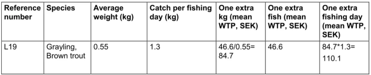
According to this conversion procedure the three changes “one extra kilo”, “one extra fish” and “one extra fishing day” have been given a common unit as each change can be converted to weight. A numerical example of how the conversion has been performed in practice follows below. The study (reference number: L19) in Table 2 below has estimated the mean willingness to pay for grayling and brown trout. These species were stated in the study, and using Carlstrand’s mean weight figures (grayling: 0.3 kg and brown trout: 0.8 kg) their average weight has been calculated as 0.55 kg. The catch per fishing day is calculated from Swedish Board of Fisheries (2009) and is estimated at 1.3 kg.