1
Institutional and structural change – effects on
employment and house prices on local markets in
Sweden 1985–2014
Work in progress dated 2017-05-09
Peter Håkansson1,2 and Magnus Andersson1
1 Department of Urban Studies, Malmö University, SE-205 06 Malmö, Sweden 2 Corresponding author, peter.hakansson@mah.se
2
Institutional and structural change – effects on employment and house prices on local markets in Sweden 1985 – 2014.
Introduction
There are many examples of when economic structural change leads to asymmetrical local growth and inequality between regions. The literature on regional development and inequality is popular with terms related to geography, such as region, spatiality, locality, proximity, district, local context, and
neighbourhood effects (Wei, 2015). The literature suggests that the reason for asymmetric local growth is that economic structural change affects municipalities and districts differently (Martin, 2011). Further, local growth has been of focus in a selection of disciplines using different theoretical and
methodological approaches; from regional planning and economic geography focusing cities as
agglomeration and drivers of growth (Krugman, 1991; Wu, & Chen, (2015), labor markets (Suedekum, Wolf, & Blien, 2014), human capital (Gennaioli et al., 2013), the relationship between real estate prices and accessibility (Du & Mulley, 2012). The problem of measuring socio-economic development on a local level has stimulated research in many different disciplines (i.e. economic geography, economic history), for many decades (Barro 1991; Gallup et al. 1999; Maddison 1995).
It may seem natural that in a transition process, municipalities and regions develop diversely, i.e. unemployment will increase in a region that lag behind, but decrease in regions that benefit on the transition process. In neoclassical theory, this will even out over time due to wage differentials and mobility. In a region with an increasing demand for labour, wages will rise and the opposite will happen in a region with decreasing demand for labour. However, these inequalities between regions sometimes seem to be persistent.
Local labour markets have been analysed in numerous studies in recent years, for example in relation to cultural diversity (Suedekum, Wolf, & Blien, 2014), mobility, overeducation and educational mismatch (Croce & Ghignoni 2015; Ramos & Sanromá, 2013), and trade and technology (Autor, Dorn & Hanson, 2015). Even though mobility in different forms is central in these studies, mobility still becomes a one-dimensional factor. Concerns like housing prices, public transport or other factors that may be central for mobility of the individual is seldom or never analysed.
Another thread in the research has been spatial mismatch hypothesis (SMH). The research derives from Kain’s (among others Kain, 1968) research on discrimination of African-Americans in in wealthy neighbourhoods. The hypothesis is that the closer you live to the location of jobs, the higher probability
3
to have a job, and because African-Americans are discriminated in wealthy neighbourhoods were the jobs are located, unemployment is higher in these groups. Conclusively, improving spatial access to jobs would lead to better outcomes on employment among African-Americans. However, even though SMH highlights the importance of accessibility, fairly little has been done on how the house market works (beyond discrimination), even though transportation has been highlighted with this stream of research. Further, change, and specifically, structural change has not been highlighted within this stream of research.
Further, institutional change may affect spatial inequality. North (1990) defines institutions as “the rule of the game”. According to North (1990, 2005) there are both formal institutions (laws and regulations) and informal constraints - or institutions - (norms and tradition). According to North, institutions can be defined as “the constraints that human beings impose on human interaction” (North, 2005, p. 59). Conclusively, institutional change could be changes in rules and regulations, for example new laws that concerns housing or as mentioned above, a government policy on improving spatial access to jobs, but it could also be a change in norms.
The aim of this paper is to highlight how institutional and structural change has affected municipalities in Sweden when it comes to employment and housing. For this, we use official data from Statistics Sweden on house prices and employment. Data is on municipality level and covers thirty years, 1985– 2014. The research question then becomes: In relation to employment and house prices, which
municipalities has gained and which has lost from institutional and structural change during this period? Which municipalities has managed to adopt, and which has not?
The perspective in this paper is that the rate of employment on a local labour market is affected by mobility. The idea that mobility affect employment is far from new. Already Friedman (1968)
emphasized the role of mobility, but also the Swedish Rehn-Meidner model is constructed on the idea that mobility can have a positive influence on the labour market, and specifically, if mobility is high, both unemployment as well as inflation could be kept on lower levels. Further, we claim that mobility can be hindered by the local housing market. This connection between unemployment and the housing market has, however, been less explored, but there are exceptions. Dohmen (2005), for example, studies home ownership and unemployment from the perspective that with home ownership follows higher moving costs and therefore home ownership leads to less mobility and higher unemployment. In addition, Lux & Sunega (2012) comes to this conclusion in a study on the Czech Republic. Within the
4
Czech Republic, the post-socialist policy has been to privatize public housing and to encourage householders to buy their house. As Lux & Sunega point out “…if governments pursue a policy of increasing homeownership, this may have the unintended consequence of making specific labour segments less mobile” (Lux & Sunega, 2012, p. 501).
Even though, there are an important relationship between housing and the labour market, these two markets have less often been integrated into one simultaneous model. In this paper, we develop a conceptual model where the labour and the housing markets interact. We consider four regions with a high demand on the labour market (employment rate above average) and housing market (house prices above average) or low demand on these markets simultaneously. In this non-equilibrium model, long-term low employment rate (and high unemployment or inactivity) would be possible due to costs of moving, low wage differentials and insufficient institutional arrangements. However, what we are interested of in this paper is how high and low demand on labour respectively housing has varied between different periods.
This paper is structured as follows: In the next section, the conceptual model will be outlined. This simple model is a taxonomy in two dimensions: local labour markets and local housing markets. The aim with the model is to show how non-equilibrium situation can exist side by side. For example, one local market may experience a high demand on the labour market, while another experience a low demand, and this situation may persist over time. This also goes for the housing market.
In the section after, we discuss structural change in Sweden from a Schumpeterian structural analytical perspective. We use the structural periods for Sweden suggested by Schön (2007; 2009). By structuring the years 1985–2014 in periods of structural change, and combining these periods with geographic areas, this will give us a possibility to study how structural change has affected different parts of Sweden and if structural change has led to divergence or convergence between local markets during these periods. Further, this periodization could also be used to discuss major reforms on the housing market in Sweden, which is discussed in the section after. In Sweden, these were the Income Tax Reform 1990–1991 and the reduction of subsidies in the beginning of the 1990s.
In the fifth section, we discuss data and show our results. Data is presented descriptively in maps and analysed by studying convergence/divergence by comparing variation in the data for the different periods. The paper ends with a discussion on how institutional and structural change may have
5
contributed to divergence between regions, but also, as in some cases, why some local labour markets seem to converge.
A conceptual model
The following conceptual model considers a neoclassical model with four regions with either high demand on the labour market (employment above average) and housing market (house prices above average) or low demand1 on these markets simultaneously. A third and fourth situation would be high
demand on one market and low demand on the other, as figure 1 shows.
Figure1: A conceptual model of non-equilibrium on two markets simultaneously.
Labour market
High demand Low demand
H ous ing m ar ke t
High demand Local labour market 1 Employment rate above average
House prices above average
Local labour market 2 Employment rate
below average
House prices above average
Low demand Local labour market 3
Employment rate above average
House prices below average
Local labour market 4 Employment rate
below average
House prices below average
1 For a clarification: By “high demand” we mean a demand above average, and “low demand” is, consequently, below
6
To begin with, we consider completely flexible prices and lack of mobility. Low mobility can be caused by high costs of moving or regulated mobility by the authorities. With flexible prices, wages and house prices would adapt to a new equilibrium before people started to move. On the other hand, if prices (wages and house prices) are sticky, but the cost of moving relatively low (and mobility is allowed by authorities) people will move (or commute), which will result in an equilibrium on each local labour market, but also in an equilibrium on the total, national labour market.
The third situation, the non-equilibrium situation, is the situation when the cost of moving (or
commuting) exceeds the gains. Here the housing market becomes important. For example, net losses on selling houses/apartments in a situation with excess supply (and decreasing prices), could be considered as a moving cost. If people not are prepared to take this cost, we will have a permanent non-equilibrium situation.
Consider local labour market 1. This is a local labour market in expansion and has moved into highly productive areas and need labour; both high-skilled as well as in low-skilled service positions.2 When
there is an excess demand for labour, we know that wages will increase. Because it is an area in rapid expansion, both demographically as well as economically, there will be an excess demand for housing. Because of this excess demand, house prices will increase.
The opposite of the local labour market 1 is labour market 4. This is a region that lags behind in the economic structural transition. Unemployment is high and there is an excess supply on the housing market because people are getting poorer, but also because people are moving out from the region. If people would move from local labour market 4 to 1, they would do a net loss on their house, but they would also have to pay more for new housing in their new region. The conditions on the housing market therefore hinder a move from local labour market 4 to 1.
A different and more advantageous situation would be for unemployed people living in local labour market 2. If they own a house they may sell it to a net profit and to a lower cost move to local labour market 1. The most attractive local labour markets would probably be local labour market 3. Here there
2 There is an ongoing discussion on how the new knowledge and service society has been polarized and that an increase in
high-skilled jobs lead to an increase in low-skilled service jobs, so called “high-touch jobs” like waitressing, cleaning, caring and serving. This will be discussed later.
7
is a demand for labour but still excess supply of houses. If so, there would be a flow of labour into this local labour market and house prices would soon start to increase.
Conclusively, there are two local labour markets (2 and 3) where some sort of equilibrium on the labour market would be possible to reach. For local labour markets 1 and 4, a persistent non-equilibrium state is the most likely situation.
There are several examples from countries that experience structural and spatial change where increasing demand for housing lead to bottlenecks in the urban and regional development. Housing prices has attracted increasing public attention in line with the growth of a commercial housing market replacing the old welfare housing supply system. For example, the commercial housing market has become an important source of housing provision for urban residents in China (Chen et al., 2011). In addition, the demand for housing in China has experienced a rapid increase because of the accelerated urbanization driven by rapid economic growth and increased migration from rural regions into cities (Song & Zenou, 2012). The rapid demand for housing provides raising housing prices in Chinese cities, especially large and medium-sized cities have risen substantially (Ren et al., 2012). Compared to household income, housing is unaffordable to a large proportion of urban residents, which tends to become a serious social problem in China (Chen et al., 2011; Li, 2012). Housing price ranked second in 2013 (top one from 2007 to 2012) as one of the most pressing public social problems in China (Ren et al. 2012). Chinese housing prices as an example on the problems of middle-income trap and spatial inequality Zhang, & Tang, (2016).
Structural change
One way of analysing structural change is to use Lennart Schön’s Schumpetarian concept (see for example Schön 2009, 2007). In this approach, technical innovation is central and the creation of new complementarities around macro innovations. The structural cycle can, according to the concept, be accrued in two growth periods interrupted by crises. The first growth period is characterised by
transformation. This period is around 20–25 years long. During this period, development is uneven and unbalanced. The second period is characterised by rationalisation. During this period, growth
8
After the last Swedish structural crises (1975–1980) followed the so-called third industrial revolution, when the microchip and its complementarities started a new technological wave. According to Schön’s concept, there was a transformational period of structural changes from the late 1970s up to the
beginning of the 1990s, which was follow by a transformational crisis in the beginning of the 1990s. From mid 1990s, Sweden has experienced an exceptional growth rate with a doubling of the growth, which indicate that Sweden had experienced the rationalisation phase the last 15 years. We should around 2010 be in the end of this rationalisation period, facing a structural crisis. In relation to the tendencies on the labour market, this seems reasonable.
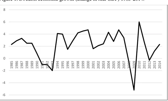
Swedish economy 1985–2014
As figure 1 shows, Swedish economy was hit by major recessions twice during the period. The first one, characterized as a transformational crisis in Schön’s definition, coincide with the European “ecu-crisis” in the beginning of the 1990s. The second major drop in economic growth coincide with the Great Recession and the international financial crises 2008–2009. According to Schön’s concept and periodization, this crisis could be categorized as a structural crisis.
Figure 1: Swedish economic growth (change in real GDP) 1985-2014.
Source: National Institute of Economic Research [Konjunkturinstitutet], Forecast Database.
-6 -4 -2 0 2 4 6 8 1985 1986 1987 1988 1989 1990 1991 1992 1993 1994 1995 1996 1997 1998 1999 2000 2001 2002 2003 2004 2005 2006 2007 2008 2009 2010 2011 2012 2013 2014
9
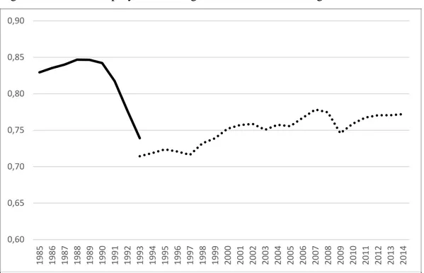
The two major recession over this period affected employment and the labour market quite differently. As figure 2 shows, employment dropped severely in the 1990s recession, but minor during the Great Recession 2008–2009, even though GDP dropped more during the Great Recession.
Figure 2: Swedish employment rate age 20-64. National average.
Source: Statistics Sweden, ÅRSYS and RAMS.
However, what has changed over time is the rate of employees in service and manufacturing. Figure 3 shows how structural change has affected the sectors service and manufacturing. From 1990 to 2014, the share of employed in the service sector (not incl. education and healthcare) has increased from around 35 percent to around 45 percent. On the other hand, the share of employees in manufacturing has decreased over the same period from 20 percent to 12 percent. Further, even though there are a long-term trend over the last fifteen years towards the service economy, we can see a “jump” upwards (in the service curve) and downwards (in the manufacturing curve) during the Great Recession. During the recession in the beginning of the 1990s, we can observe a minor drop in manufacturing, but no related upturn in service. 0,60 0,65 0,70 0,75 0,80 0,85 0,90 1985 1986 1987 1988 1989 1990 1991 1992 1993 1994 1995 1996 1997 1998 1999 2000 2001 2002 2003 2004 2005 2006 2007 2008 2009 2010 2011 2012 2013 2014
10
Figure 3: Number of employed in service (not incl. education and healthcare) and manufacturing in relation to total number of employed. Sweden, 1990 – 2014.
Source: Statistics Sweden, RAMS.
Conclusively, due to the drop in production and employment and the change in production structure, we argue for a periodization in three periods. The first period (1985–1992) cover a transformation period and ends with the transformational crisis 1992–1993. The second one (1993–2008) is a rationalization period and ends with the structural crisis 2008–2009. The last period can be considered as a period after the Great Recession.
Institutional change
The Swedish real estate market has undergone severe institutional change during the last 50 years. During the period studied in this article, a reform of major importance was Income Tax Reform 1990-1991. Further, during the beginning of the 1990s, the Liberal/Conservative Government lowered the housing subsidies. These reforms coincide with the recession in the beginning of the 1990s.
0,0% 5,0% 10,0% 15,0% 20,0% 25,0% 30,0% 35,0% 40,0% 45,0% 50,0% 1990 1991 1992 1993 1994 1995 1996 1997 1998 1999 2000 2001 2002 2003 2004 2005 2006 2007 2008 2009 2010 2011 2012 2013 2014 Service Manufacturing
11
Data and results
Our analysis derives from the conceptual model described above, where we use a taxonomy with four different non-equilibrium situations. To visualize and exemplify this model we use official data from Statistics Sweden on house prices and employment rate (age 20–64) on municipality level. We
standardize the data from each single municipality (per year) with the national average. For employment rate this is calculated as follows:
𝑠𝑠𝑖𝑖𝑖𝑖 = 𝑙𝑙𝑙𝑙𝑖𝑖𝑖𝑖𝑖𝑖
where
i = municipality l = employment rate t = year
House prices are managed the same way. This gives us a standardized rate that could be above 1 (employment rate or house prices above the national average) or below 1 (below national average). We have accrued the data into three periods in accordance with the structural cycles discussed above. For this, we have calculated averages for each municipality over the period on each variable
respectively. We have combined the variables in accordance with the conceptual model in Figure 4 and this is presented descriptively in three maps corresponding to the periods 1985-1992, 1993-2008 and 2009-2014.
12 Figure 4: The conceptual model in Sweden 1985 - 2014
The maps in figure 4 show a concentration of the prosperous municipalities over time. In the period 1985–1992 the municipalities with both an employment rate, as well as house prices above average (red colour on the map) is more spread out over the country. In 2009 – 2014, there is no such municipality above the Stockholm region. One municipality that seems to stand out, however, is Jönköping, which can be considered as an urban centre in the middle of Småland.
When it comes to the Stockholm region, we can see a concentration. The “red” municipalities where more spread out in the Stockholm region in the first period, but concentrated more towards Stockholm City in the last period. It is interesting to notice that Norrtälje, north of Stockholm, move from housing prices above average to below average after 2008, but the employment rate is still above average. In Western Skåne and Halmstad we can see that house prices increase to a situation above average over the period, but we can also see an increase in employment rates in some cases. Halmstad, for example move
13
from a situation with employment rate and house prices below average in the first period, to the opposite in the last period.
For the part of the country above Stockholm (Norrland) we move from a situation mainly below average, both on employment rate and house prices (grey colour), to a situation with still low (or decreasing) house prices, but with employment rate above average. Two municipalities (Östersund and Falun) moves from a situation with house prices above average in the first period to a situation below average after 1992. However, employment rate is above average in all periods in these two
municipalities.
In general, we can see that the green and the red coloured municipalities are less than the grey and the yellow coloured, and this difference seems to increase over time (the green and the red become fewer). This may implicate that we see a polarization when it comes to house prices; municipalities with house prices above average are in the last period mainly concentrated to the west coast and the Stockholm region. A majority of the municipalities experience house prices below average, which must mean that in municipalities with house prices above average, the prices are far above.
Testing the emergence of increased divergence for employment rates and house prices
The maps in figure 4 provides a visual pattern of increased divergence between Swedish municipalities. The divergence of labour and real estate markets are analyzed in Figures 6–8. The figures builds on the conceptual model presented earlier. Municipalities above the horizontal axis experience house prices above average and municipalities under the axis experience house process below average. For
employment, the municipalities to the left of vertical axis experience higher rates than the average and to the right lower rates that average.
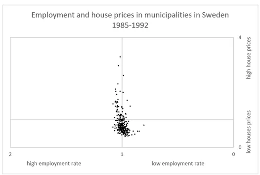
The first period, 1985–1992, the majority of municipalities are clustered in the middle of the diagram indicating a homogenous relationship between employment and low house prices. For the second period, 1993–2008, there is a larger dispersion among the municipalities with an increasing number of
municipalities with high house prices and high employment rates but also general trend with decreasing house prices. For the third period, a divergence is evident.
14 Figure 5: Employment and house prices 1985-1992
15 Figure 7: Employment and house prices 2009-2014
What if there are significant differences within the three periods that we wish to test for equality of variance? The test conducted is that of Levene (1960) (labeled as W0 below), which is robust to non-normality of the error distribution. Two variants of the test proposed by Brown and Forsythe (1974), which uses more robust estimators of central tendency (e.g., median rather than mean) are also computed. We apply the test to the municipality data series to examine whether the variance of the population is constant across the time periods for each of the two variables; employment rate and house price. The test reports Levene’s robust test statistic (W0) for the equality of variances between the three periods using the mean and the two statistics proposed by Brown and Forsythe that replace the mean in Levene’s formula with alternative location estimators. The first alternative (W50) replaces the mean with the median. The second alternative replaces the mean with the 10% trimmed mean (W10).
16 Table 1: Robvar Employment by Period 1 to 3
Period | Mean Std. Dev. Freq. ---+--- 1 | .99934999 .03638318 280 2 | 1.0167577 .0498756 280 3 | 1.0173105 .05045612 280 ---+--- Total | 1.0111394 .04672923 840 W0 = 12.867218 df(2, 837) Pr > F = 0.00000313 W50 = 12.896311 df(2, 837) Pr > F = 0.00000305 W10 = 12.884615 df(2, 837) Pr > F = 0.00000308
Table 1 shows that the test clearly reject the hypothesis of equal variance across the time periods for the employment rates in Swedish municipalities. The increased standard derivation from period 1 to 3 illustrates the divergence occurring during the early 1990 in the Swedish economy in local labour markets.
Table 2: Robvar House prices by Period 1 to 3
Period | Mean Std. Dev. Freq. ---+--- 1 | .87256151 .40279243 280 2 | .76727225 .48461694 280 3 | .71351242 .54386837 280 ---+--- Total | .78444873 .48454201 840 W0 = 8.3498008 df(2, 837) Pr > F = 0.0002567 W50 = 4.6066082 df(2, 837) Pr > F = 0.01024015 W10 = 6.2687891 df(2, 837) Pr > F = 0.00198467
Table 2 provides a similar pattern however, the changes in the standard derivation between the period are more equally distributed, even if they significantly differ. The results of the test show divergence over time on both local markets; local labour markets as well as local housing markets.
17
Discussion and conclusions
The present study highlights how structural and institutional change affect spatial inequality within two interlinked markets, labour market and the housing market over time
These results show the importance of local markets characteristics. Structural and institutional change could favour or disfavour a local market. Our analysis indicate increasing divergence between Swedish municipalities over the period 1985 to 2014. However, the magnitude of the divergence differs within the studied period showing stronger effects during the early periods.
Despite its preliminary nature, this paper attempts to be innovative in relation to asymmetrical local growth. By shedding some light on the causes and the nature of non-equilibrium of two markets with different demand and supply of housing and employment opportunities, the paper provides a conceptual framework to analyse the spatial outcome of two markets.
References
Autor, D. H., Dorn, D., & Hanson, G. H. (2015). Untangling trade and technology: Evidence from local labour markets. The Economic Journal, 125(584), 621-646. doi:10.1111/ecoj.12245
Bartholomew, Keith, and Reid Ewing. (2011). Hedonic price effects of pedestrian-and transit-oriented development. Journal of Planning Literature 26.1: 18-34.
Baum-Snow, N., & Kahn, M. E. (2000). The effects of new public projects to expand urban rail transit. Journal of Public Economics, 77(2), 241-263.
Brown, M. B., and A. B. Forsythe. (1974). Robust tests for the equality of variances. Journal of the
American Statistical Association 69: 364–367.
Cai, F. (2012). Is There a “Middle‐income Trap”? Theories, Experiences and Relevance to China. China
& World Economy, 20(1), 49-61.
Cervero, R., & Duncan, M. (2002). Benefits of proximity to rail on housing markets: experiences in Santa Clara County. Journal of Public Transportation,5(1).
Chen, J., Guo, F., & Wu, Y. (2011). One decade of urban housing reform in China: urban housing price dynamics and the role of migration and urbanization, 1995 to 2005. Habitat International, 35(1).
18
Croce, G., & Ghignoni, E. (2015). Educational mismatch and spatial flexibility in Italian local labour markets. Education Economics, 23(1), 25-46. doi:10.1080/09645292.2012.754121
Debrezion, G., Pels, E., & Rietveld, P. (2011). The impact of rail transport on real estate prices an empirical analysis of the dutch housing market. Urban Studies, 48(5), 997-1015.
Dickerson, A. M. (2005). Caught in the Trap: Pricing Racial Housing Preferences. Michigan Law
Review, 103, 101.
Dohmen, T.J. (2005). Housing, mobility and unemployment. Regional Science and Urban Economics, 35 (2005), 305–325.
Du, H., & Mulley, C. (2012). Understanding spatial variations in the impact of accessibility on land value using geographically weighted regression. Journal of Transport and Land Use, 5(2).
Friedman, M., (1968). The role of monetary policy. American Economic Review, 58 (1), 1–17.
Gennaioli, N., & La Porta, R. F. Lopez-de-Silanes, and A. Shleifer (2013). Human Capital and Regional Development. Quarterly Journal of Economics, 128(1), 105-164.
Hess, D. B., & Almeida, T. M. (2007). Impact of proximity to light rail rapid transit on station-area property values in Buffalo, New York. Urban studies,44(5-6), 1041-1068.
Jiang, B., & Yao, X. (2010). Geospatial analysis and modeling of urban structure and dynamics: an overview. In Geospatial Analysis and Modelling of Urban Structure and Dynamics (pp. 3-11). Springer Netherlands.
Kain, J. F. (1968). Housing Segregation, Negro Employment, and Metropolitan Decentralization. The
Quarterly Journal of Economics, (2). 175.
Kohli, H. A., & Mukherjee, N. (2011). Potential costs to Asia of the middle income trap. Global Journal
of Emerging Market Economies, 3(3), 291-311.
Krugman, P. (1990). Increasing returns and economic geography (No. w3275). National Bureau of Economic Research.
Levene, H. (1960). Robust tests for equality of variances. In Contributions to Probability and Statistics:
Essays in Honor of Harold Hotelling, ed. I. Olkin, S. G. Ghurye, W. Hoeffding, W. G. Madow, and H.
B. Mann, 278–292. Menlo Park, CA: Stanford University Press.
Li, S.-m. (2012). Housing inequalities under market deepening: the case of Guangzhou, China.
Environment and Planning-Part A, 44(12).
Lux, M. and Sunega, P. (2012). Labour Mobility and Housing: The Impact of Housing Tenure and Housing Affordability on Labour Migration in Czech Republic. Urban Studies, 49(3), 489–504. Martin, R. (2011). The local geographies of the financial crisis: from the housing bubble to economic recession and beyond. Journal of Economic Geography, 11(4), 587-618.
19
North, D.C. (2005). Understanding the process of economic change. Princeton, N.J.: Princeton University Press,.
North, D.C. (1990). Institutions, Institutional Change and Economic Performance. Cambridge: Press Syndicate of the University of Cambridge.
Ohno, K. (2009). Avoiding the middle-income trap: renovating industrial policy formulation in Vietnam. ASEAN Economic Bulletin, 26(1), 25-43.
Ramos, R., & Sanromá, E. (2013). Overeducation and local labour markets in spain. Tijdschrift Voor
Economische En Sociale Geografie, 104(3), 278. doi:10.1111/j.1467-9663.2012.00752.x
Schön, L. A. (2009). Technological Waves and Economic Growth - Sweden in an International Perspective 1850-2005. Circle Electronic Working Paper Series, paper no. 2009/06.
Schön, L. (2007). En modern svensk ekonomisk historia: tillväxt och omvandling under två sekel. (2., [rev.] uppl.) Stockholm: SNS förlag.
Song, Y., & Knaap, G. J. (2004). Measuring the effects of mixed land uses on housing values. Regional Science and Urban Economics, 34(6), 663-680.
Song, Y., & Zenou, Y. (2012). Urban villages and housing values in China. Regional Science and Urban
Economics, 42(3).
Suedekum, J., Wolf, K., & Blien, U. (2014). Cultural diversity and local labour markets. Regional
Studies, 48(1), 173-191. doi:10.1080/00343404.2012.697142
Wei, Y. D. (2015). Spatiality of regional inequality. Applied Geography, 61, 1-10.
Wu, J., & Chen, Y. (2015). The Evolution of Municipal Structure. Journal of Economic Geography, lbv022.
Zhang, Z., & Tang, W. (2016). Analysis of spatial patterns of public attention on housing prices in Chinese cities: A web search engine approach. Applied Geography, 70, 68-81.