Dynamic analysis of soil-steel composite railway bridges: FE-modeling in Plaxis

(1)

Dynamic analysis of soil-steel

composite railway bridges

FE-MODELING IN PLAXIS

OROD AAGAH & SIAVASH ARYANNEJAD

KTH ROYAL INSTITUTE OF TECHNOLOGY

(2)

(3)

Dynamic analysis of soil-steel

composite railway bridges

FE-modeling in Plaxis

O

ROD

A

AGAH

S

IAVASH

A

RYANNEJAD

Master of Science Thesis

Stockholm, Sweden 2014

(4)

i TRITA-BKN. Master Thesis 436, 2014 ISSN 1103-4297

ISRN KTH/BKN/EX-436-SE

KTH School of ABE SE-100 44 Stockholm SWEDEN © Orod Aagah & Siavash Aryannejad 2014

Royal Institute of Technology (KTH)

Department of Civil and Architectural Engineering Division of Structural Engineering and Bridges

(5)

i

Abstract

A soil-steel composite bridge is a structure comprised of corrugated steel plates, which are joined with bolted connections, enclosed in friction soil material on both sides and on the top. The surrounding friction soil material, or backfill, is applied in sequential steps, each step involving compaction of the soil, which is a necessity for the construction to accumulate the required bearing capacity. Soil-steel composite bridges are an attractive option as compared with other more customary bridge types, owing to the lower construction time and building cost involved. This is particularly true in cases where gaps in the form of minor watercourses, roads or railways must be bridged. The objective of this master thesis is the modelling of an existing soil-steel composite railway bridge in Märsta, Sweden with the finite element software Plaxis. A 3D model is created and calibrated for crown deflection against measurement data collected by the Division of Structural Engineering and Bridges of the Royal Institute of Technology (KTH) in Stockholm, Sweden.

Once the 3D model is calibrated for deflection, two 2D models with different properties are created in much the same way. In model 1, the full axle load is used and the soil stiffness varied, and in model 2 the soil stiffness acquired in the 3D model is used and the external load varied. The results are compared to measurement data.

In 2D model 1 an efficient width of 1,46 m for the soil stiffness is used in combination with the full axle load, and in 2D model 2 an efficient width of 2,85 m is used for the external load, in combination with the soil stiffness acquired in the 3D model.

Aside from this, parametric studies are performed in order to analyse the effect of certain input parameters upon output results, and in order to analyse influence line lengths.

Recreating the accelerations and stresses in the existing bridge using finite element models is complicated, and the results reflect this. Below are shown the discrepancies between model results and measurement data for the pipe crown. The scatter in the measurement data has not been taken into consideration for this; these specific numbers are valid only for one particular train passage.

For crown deflection, the 3D model shows a discrepancy of 4%, 2D model 1 5% and 2D model 2 8% compared with measurement data. For crown acceleration, in the same order, the discrepancy with measurements is 1%, 71% and 21% for maximum acceleration, and 46%, 35% and 28% for minimum acceleration. For maximum crown tensile stress, the discrepancy is 95%, 263% and 13%. For maximum crown compressive stress, the discrepancy is 70%, 16% and 46%.

(6)

ii

Keywords: Soil-steel composite bridge, Corrugated steel culvert, High-speed railways, FEM, Plaxis, Field measurements

(7)

iii

Sammanfattning

En rörbro av stål är en konstruktion av korrugerade, ihopskruvade plåtar som är kringfylld av friktionsmaterial på sidorna och ovantill. Det omkringliggande friktionsmaterialet, eller kringfyllningen, appliceras och kompakteras lagervis, vilket är en nödvändighet för att konstruktionen ska få nödvändig bärförmåga. Rörbroar är ett attraktivt alternativ jämfört med mer traditionella brotyper, med anledning av kortare konstruktionstider- och kostnader. Detta är speciellt sant i de fall där mindre vattendrag, vägar eller järnvägsspår ska korsas.

Målsättningen med denna masteruppsats är modellering av en befintlig rörbro för järnvägstrafik i Märsta med finitia elementprogrammet Plaxis. En 3D-modell skapas och kalibreras för nedböjning i hjässa mot mätdata som insamlats av Avdelningen för Bro- och Stålbyggnad vid Kungliga Tekniska Högskolan i Stockholm, Sverige.

När 3D-modellen kalibrerats för nedböjning i hjässa skapas två 2D-modeller på liknande sätt. I ena används den totala axellasten och jordens styvhet varieras, och i andra används den styvhet för jorden som erhålls i 3D-modellen medan den externa lasten varieras. Resultaten jämförs med mätdata.

I 2D modell 1 används en effektiv bredd på 1,46 m för jordstyvheten i kombination med den totala axellasten, och i 2D modell används en effektiv bredd på 2,85 meter för den externa lasten, i kombination med den jordstyvhet som erhålls i 3D-modellen. Utöver detta görs parametriska studier för att analysera effekten av vissa indata på modelleringsresultaten, och för att analysera influenslinjelängder.

Att åteskapa accelerationer och spänningar i den befintliga rörbron genom användandet av finita element modeller är komplicerat, och resultaten återspeglar detta. Nedan visas skillnaderna mellan resultat från modellen och mätdata för rörets hjässa. Hänsyn har inte tagit till spridningen i mätdata för detta; dessa specifica siffror är endast gällande för ett särskilt tågpassage.

För nedböjning I hjässa visar 3D modellen en skillnad på 4%, 2D model 1 5% och 2D model 2 8% jämfört med mätdata. För acceleration i hjässa, i samma ordning, är skillnaden mot mätdata 1%, 71% och 21% för högsta acceleration, och 46%, 35% och 28% för minsta acceleration. För högsta dragspänning i hjässa är skillnaden 95%, 263% och 13%. För högsta tryckspänning i hjässa är skillnaden 70%, 16% och 46%.

Nyckelord: Samverkanskonstruktion, Rörbro, Korrugerad stålplåt, Höghastighetståg, FEM, Plaxis, Fältmätning

(8)

(9)

v

Preface

The authors would like to thank a number of persons whose help and encouragement over the course of the spring and summer of 2014 was greatly appreciated.

Our genuine thanks to Professor Raid Karoumi, Head of Division of Structural Engineering and Bridges at the Royal Institute of Technology, Stockholm, for giving us the chance to take part of this stimulating subject and to write our master thesis around it. Our heartfelt thanks also to our supervisors, Andreas Andersson, Researcher, Ph.D, and Lars Pettersson, Adj. Professor, for all their help and support and for giving us a push when we needed it.

We would like to thank the following persons at Ramböll Geoteknik, Stockholm; Anders Westin, Head of Department, for allowing us to write our master thesis at Ramböll and David Rósenkrans Hauksson and Abdennour Hamis, for providing their generous support.

Finally, we would like to thank our loving families for standing by our sides always. Without them none of this would have been possible. The conclusion of this part of our lives is so much the sweeter for having you all to share it with.

Stockholm, July 2014

Orod Aagah

(10)

(11)

vii

List of Figures

Figure 1.1: Culvert being lifted onto site and backfilling being applied [4]. ... 2

Figure 1.2: Figure 6.9 of EN 1991-2. ... 3

Figure 2.1: Bridge location, 40 km north of Stockholm. ... 9

Figure 2.2: The X52-train passing over the bridge[6] ... 10

Figure 2.3: X52 axle distances [6]. ... 10

Figure 2.4: Section of the construction in the direction of the tracks[13]. ... 11

Figure 2.5:Plan view of the bridge [13]. ... 11

Figure 2.6: Section through longitudinal direction of the pipe [6] ... 12

Figure 2.7: Section of pipe beneath track centre [6]. ... 12

Figure 2.8: Detail of positions of strain gauges on the inside of the corrugated steel plate [6]. ... 13

Figure 2.9: Measurement data for crown. Deflection, acceleration, stress in corrugation valley and stress in corrugation crest. ... 13

Figure 2.10: Max vertical crown displacement d1 and d2 for all train passages [6]. .... 14

Figure 2.11: Max vertical acceleration during train passages, all signals have been subjected to a 30 Hz low-pass filter [6]. ... 14

Figure 2.12: Measured train induced stresses, a) proportions of bending and axial stress at peak stress for one X52 passage, b) corresponding proportions using gauge e5-e6 (at the crown) for all recorded train passages [6]. ... 15

Figure 3.1: 3D model before calculation. ... 18

Figure 3.2: 2D model 1 (above) and 2D model 2 (below) before calculation. ... 18

Figure 3.3: 3D soil geometry after insertion of boreholes ... 20

Figure 3.4: a) polycurve for elliptical pipe section, b) 3D model pipe. ... 23

Figure 3.5: Local system of axes for beams as specified in section 6.6.2 of [17]. ... 24

Figure 3.6: Load multiplier 3. ... 27

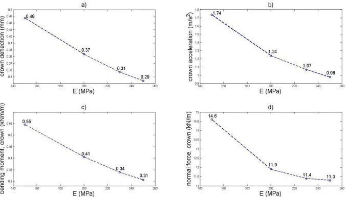
Figure 3.7: Crown results for mesh number five in 3D. a) vertical crown deflection, b) vertical crown acceleration, c) crown bending moment and d) crown normal force. .... 31

Figure 3.8: Quotas of max deflection, acceleration and section forces in the crown for the five different meshes, as compared with mesh number five. ... 32

Figure 3.9: Crown results for mesh number four in 2D. a) vertical crown deflection, b) vertical crown acceleration, c) crown bending moment and d) crown normal force. .... 34

Figure 3.10: Quotas of max deflection, acceleration and section forces in the crown for the five different meshes, as compared with mesh number five. ... 35

Figure 3.11: 3D geometry, dynamic phase. ... 37

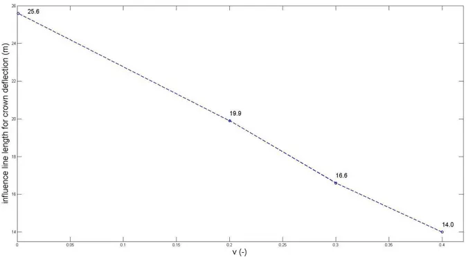
Figure 3.12: 2D geometry, dynamic phase. Upper part shows model 1, lower model 2. 37 Figure 4.1: Crown deflection influence line lengths for different values of poisson’s ratio. ... 40

(16)

xii

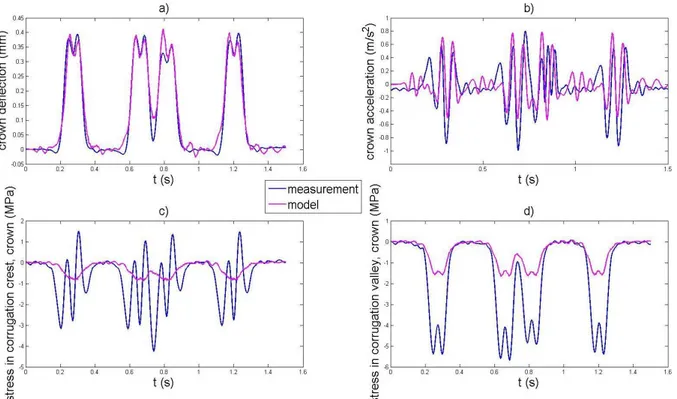
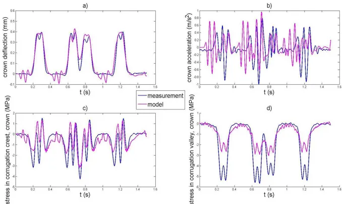
Figure 4.2: Pipe crown results versus measurement data. a) vertical deflection, b) vertical acceleration, c) stress in corrugation crest and d) stress in corrugation valley. ... 42 Figure 4.3: Maximum pipe crown results, varied soil stiffness. a) vertical deflection, b) vertical acceleration, c) bending moment and d) normal force. ... 43 Figure 4.4: Maximum pipe crown results, low friction between pipe and backfill. a) vertical deflection, b) vertical acceleration, c) bending moment and d) normal force. . 44 Figure 4.5: Model 1 influence line lengths for crown. a) vertical deflection, varied soil stiffness, b) bending moment, varied soil stiffness c) vertical deflection, varied poisson’s ratio and d) bending moment, varied poisson’s ratio. ... 45 Figure 4.6: Model 2 influence line lengths for crown. a) vertical deflection, varied soil stiffness, b) bending moment, varied soil stiffness c) vertical deflection, varied poisson’s ratio and d) bending moment, varied poisson’s ratio. ... 46 Figure 4.7: Pipe crown results versus measurement data, model 1. a) vertical deflection, b) vertical acceleration, c) stress in corrugation crest and d) stress in corrugation valley. ... 47 Figure 4.8: Pipe crown results versus measurement data, model 2. a) vertical deflection, b) vertical acceleration, c) stress in corrugation crest and d) stress in corrugation valley. ... 48 Figure 4.9: Maximum pipe crown results, varied soil stiffness. a) vertical deflection, b) vertical acceleration, c) bending moment and d) normal force. ... 49 Figure 4.10: Maximum pipe crown results, full contact and no contact between pipe and backfill. a) vertical deflection, b) vertical acceleration, c) bending moment and d) normal force. ... 50 Figure 4.11: Pipe crown results, varied load. a) vertical deflection, b) vertical acceleration, c) bending moment and d) normal force. ... 51 Figure 4.12: Comparison of 3D and 2D model results in crown, also with measurement data. a) vertical deflection, b) vertical acceleration, c) stress in corrugation crest and d) stress in corrugation valley. ... 52

(17)

xiii

List of Tables

Table 3.1: Soil properties. ... 19

Table 3.2: Borehole positions with ballast and backfill levels. ... 21

Table 3.3: 3D pipe properties. ... 22

Table 3.4: 3D sleepers and rail properties. ... 24

Table 3.5: 2D pipe and rail properties. ... 25

Table 3.6: Mesh properties, 3D. ... 30

Table 3.7: Maximum values for deflection, acceleration and section forces in the crown for 3D meshing. ... 31

Table 3.8: Mesh properties, 2D. ... 33

Table 3.9: Maximum values for deflection, acceleration and section forces in the crown for 2D meshing. ... 34

(18)

(19)

1

1 Introduction

1.1 Soil-steel composite bridges

A soil-steel composite bridge is a structure comprised of corrugated steel plates, which are joined with bolted connections, enclosed in friction soil material on both sides and on the top. The corrugated plates can be assembled into different cross sectional shapes. Some typical shapes are circular sections, elliptical sections and arched sections.

Once the steel plates have been installed, on for example concrete foundation slabs if needed, granular backfill is applied on both sides. The backfill is applied in sequential steps, each step involving compaction of the soil, which is a necessity for the construction to accumulate the required bearing capacity. The bearing capacity is thus a direct result of the interaction between the steel plates of the pipe and the friction soil surrounding it, and is also dependent upon the fill height at the crown of the conduit and the thickness of the plate itself [1]. As the structure is loaded, the deformation of the steel section is checked by the soil through the development of earth pressure as the steel is pressed against the backfill.

Soil-steel composite bridges are an attractive option as compared with other more customary bridge types owing to the lower construction time and building cost involved. This is particularly true in cases where gaps in the form of minor watercourses, roads or railways must be bridged [2]. One example demonstrating the relative ease with which this type of structure is assembled is the soil-steel composite bridge that transverses the stream Skivarpsån in southern Sweden [3]. The plates were fabricated in Canada and pieced together into an arched section with a span of about 11 m on location. The process of installing the concrete footings and the culvert and subsequently applying and compacting the backfill was completed over the course of only two days. Figure 1.1 shows the bridge being installed.

(20)

CHAPTER 1:INTRODUCTION

2

Figure 1.1: Culvert being lifted onto site and backfilling being applied [4].

1.2 Design and dynamics

Bridges are affected by dynamic loads through the passing of traffic in the form of vehicles and trains [5]. These dynamic loads affect the initial static stresses and deformations, either decreasing or increasing them. If certain conditions are met, these dynamic loads can result in a situation where they and the structure are in resonance. This means that the frequency of the excitation coincides with the natural frequency of the structure and amplifies the static stresses and deformations considerably. Other factors which can increase or decrease the static stresses and deformations are the fast frequency of loading and disparities in the load from the vehicle wheels caused for instance by flaws in the track or vehicle itself.

How the structure reacts when exposed to a dynamic load is affected by many factors [5]. Some of these are; the mass of the structure itself, the span of the bridge, the speed at which the traffic crossing it travels at, the damping inherent to the bridge, the loads in each axle along with the number and spacing of the axles and the natural frequencies of the bridge.

The effects of the dynamic loading are taken into account in the design of railway bridges according to the Eurocodes in one of two ways. Either a static analysis is carried out and the results multiplied by a dynamic factor as defined in section 6.4.5 of EN 1991-2, or a more demanding dynamic analysis is required, as specified in section 6.4.6 of the same Eurocode.

Whether a static or a dynamic analysis is required is determined with the aid of figure 6.9 (see Figure 1.2) in section 6.4.4 of EN 1991-2.

(21)

3

Figure 1.2: Figure 6.9 of EN 1991-2.

According to the Eurocode, note one in the chart above is “Valid for simply supported bridges with only longitudinal line beam or simple plate behavior with negligible skew effects on rigid supports.”

Section 6.4.3 of EN 1991-2 states the following general design rules concerning a dynamic analysis:

 The additional load cases for the dynamic analysis shall be in accordance with 6.4.6.1.2.

 Maximum peak deck acceleration shall be checked in accordance with 6.4.6.5.

 The results of the dynamic analysis shall be compared with the results of the static analysis multiplied by the dynamic factor Φ in 6.4.5 (and if required multiplied by α in accordance with 6.3.2). The most unfavourable values of the load effects shall be used for the bridge design in accordance with 6.4.6.5.

(22)

4

 A check shall be carried out according to 6.4.6.6 to ensure that the additional fatigue loading at high speeds and at resonance is covered by consideration of the stresses derived from the results of the static analysis multiplied by the dynamic factor Φ.

According to EN 1991-2 6.4.6.5 the maximum permitted peak acceleration must be lower than values given in annex A2 in EN 1990 (A2.4.4.2.1). A2.4.4.1 specifies limits of deformation and vibration when designing railway bridges. Vertical deck acceleration shall be checked to avoid instability in the ballast and to avoid excessive losses in contact forces between wheel and rail. A2.4.4.2 further specifies that the peak values in bridge deck acceleration shall not exceed 3,5 m/s2_{for ballasted tracks and 5}

m/s2 for direct fastened tracks with track and structural elements designed for high speed traffic. Frequencies shall be considered in these checks up the greater of one of three frequencies:

 30 Hz

 1,5 times the frequency of the fundamental mode of vibration of the member being considered

 The frequency of the third mode of vibration of the member

Note that these are recommended values and may be otherwise defined in the National Annex.

Furthermore, it is stated in EN 1991-2 6.4.3 that:

All bridges where the Maximum Line Speed at the Site is greater than 200 km/h or where a dynamic analysis is required should be designed for characteristic values of Load Model 71 (and where required Load Model SW/0) or classified vertical loads with α ≥ 1 in accordance with 6.3.2.

And:

For passenger trains the allowances for dynamic effects in 6.4.4 to 6.4.6 are valid for Maximum Permitted Vehicle Speeds up to 350 km/h.

Furthermore, where a dynamic analysis is required, it shall according to the flow chart be performed in conformity with the specifications of EN 1991-2 6.4.6. Section 6.4.6 regulates among other things the load combinations which shall be taken into consideration. These include Load Models HSLM, which consists of the HSLM-A and HSLM-B, the twelve Train Types specified in annex D and Real Trains specified.

Due to the complex nature of the behaviour of soil-steel composite bridges when they are subjected to loading, further insight and knowledge in how to model them in finite element software is needed in order to capture the real behaviour. Such knowledge is needed in order to produce models with which reliable dynamic analyses can be

(23)

5

performed. One important reason for this is that soil-steel composite structures operate in a way that diverges from the less complicated model of vibrating beams that is the basis for much of the norms that EN 1990 contains regarding high speed trains and dynamics [6].

1.3 Previous studies

The literature which has been read consists mainly of papers, articles and reports on full scale testing, (static and dynamic) on soil-steel composite structures, analysis of testing results and FEM-analysis of soil-steel composite bridges. In some cases only field-testing and analysis of test results have been performed, in others numerical analysis has been performed without any prior testing, and in some cases field-testing with subsequent numerical analysis and comparison has been done.

In [7], static and dynamic truck loading is performed on four soil-steel composite bridges with different sections (two box culverts and two pipe-arch culverts), spans and backfill heights. Dynamic amplification factors were calculated for these four culverts with two methods, with the difference in these two methods being how the static response was obtained. In the first method, the static response was a result of direct static testing, and in the second method the static response was in essence back-calculated using the dynamic response and filtering.

Several conclusions were made by Beben in this study. Dynamic response was higher than static response, and maximum response was observed in the conduit crown. Dynamic amplification factors (DAF) in the range of 1,105-1,293 for strains and 1,116-1,260 for displacements were calculated. Several important factors that influence the DAF were pointed out. Foremost among these were the culvert span, which causes higher DAFs as it increases. Also significant are crown soil cover height, the connection between the crown fill height and the culvert span, and the radii of the pipe. The dynamic tests were performed at speeds between 10 and 70 km/h, and it was noted that higher speeds yield higher DAFs, but with the maximum DAF acquired for a speed of 60 km/h. Another important conclusion was that the calculation of DAF by using the filtered dynamic response in order to calculate static response yields small errors. This is helpful in that such a method can be used in cases where it is not possible to perform static tests in an appropriate manner.

In [8], Beben models a soil-steel composite bridge with a box section located in Gimån, Sweden in FLAC 2D. Model calculations were compared with measured strains and deflections during the backfilling process and subsequent static vehicle loading. The model was created to mimic the construction process in that the backfill layers, all in all 20 layers, were added separately one at a time until the process was complete. In [9], static loading with trucks was performed on an arc soil-steel composite bridge with a span of 10 m and a clear height of 4,02 m. Deflections and strains were measured in different points and compared to strains and deflections calculated with

(24)

6

Cosmos/M and Robot Millenium. The measured response of the bridge was for all points lower than the calculated deflections and strains.

In [10] Kunecki and Korusiewicz perform full scale laboratory testing on a box culvert with a span of 3,55 m and a height of 1,42 m using different cover heights and load magnitudes. What they found through their testing was that the strains and displacements in the culvert were low, that the structure was very rigid and that the crown fill height had very little effect on the stiffness of the structure.

In [11], El-Sawy uses ANSYS FE-software to model two existing soil-steel culverts with the aim of comparing the results from the finite element modelling with measurement data collected by Bakht and theoretical analysis performed by Moore and Brachman for the same structures. The culverts are located in Ontario, Canada and were tested using heavy truckloads. One culvert is located in the Deux Rivieres and is circular, with a diameter of 7,77 m and a crown fill height of 2,6 m. The second culvert is located in Adelaide and has a horizontal ellipse section with a maximum width of 7,24 m and a maximum height of 4,08 m. The crown fill height is 1,35 m. According to El-Sawy, Moore and Bachman modelled the circular culvert, which is located in the Deux Rivieres, in 2D and 3D, modelling the culvert as both orthotropic and isotropic in 3D, and using plane strain and equivalent line loads to model the truckloads in 2D. The 3D models provided results for circumferential thrust, which were in line with the behaviour shown in measurements, but with overestimated values in many locations. The results from their 2D model differed from measured data and from the results of the 3D models.

El-Sawy models the Deux Rivieres culvert in two ways, once with the actual geography and once through sweeping of a 2D mesh along the longitudinal direction of the culvert. The Adelaide culvert is modelled only by the second method. The truckloads in both cases are modelled as concentrated point loads.

Equivalent thicknesses and stiffnesses in the circumferential direction are calculated based on the bending stiffness of the steel plate. For the isotropic case, the calculated equivalent thickness and Young’s modulus was the same in the longitudinal direction of the conduit, and for the orthotropic case the equivalent Young’s modulus is calculated through equating the true axial stiffness in the longitudinal direction for the corrugated plate with the equivalent stiffness in the longitudinal direction for the orthotropic plate, which according to El-Sawy satisfies both the axial and bending longitudinal stiffness’s, as opposed to the method used by Moore and Brachman, where only the axial longitudinal stiffness was satisfied.

Both soil and culvert materials are modelled as linear elastic, with two magnitudes, 30 MPa and 80 MPa, used for the soil modulus. Conclusions were made by El-Sawy that the orthotropic conduit yields results which are more in line with measurement data than does the isotropic conduit. The isotropic conduit shows values which are too high for longitudinal thrust whereas the orthotropic conduit shows negligible values, which is more in line with real behaviour. Further conclusions were made that the soil modulus does not have very strong influence on the circumferential thrusts for the

(25)

7

orthotropic case, whereas it has more of an effect on the isotropic conduit. In both cases, the soil modulus has a significant influence on circumferential bending moments. Some of the literature read concerned testing and some finite element modelling and comparing of results with measurement data. In some literature both these things were done. No literature was found that dealt specifically with soil-steel composite bridges and high speed railways, other than [12] where Mellat has performed dynamic calculations for high speed trains in the FE-software Abaqus, based on the same field-testing measurements as this study. The literature read was about further understanding the behaviour of soil-steel composite bridges, in reality and in modelling, and the extension of the knowledge we have about this kind of structure; also in connection with design norms. In this study, we, the authors, try to continue on this track in order to make some small contribution.

1.4 Aim and scope

The objective of this master thesis is the modelling of an existing soil-steel composite railway bridge in Märsta, Sweden with the finite element software Plaxis. A 3D model is created and calibrated for crown deflection against measurement data collected by the Division of Structural Engineering and Bridges of the Royal Institute of Technology (KTH) in Stockholm, Sweden.

Once the 3D model is calibrated for crown deflection, two 2D models with different properties are created in much the same way. In one the full axle load is used and the soil stiffness varied using different effective widths, and in the other the soil stiffness acquired in the 3D model is used and the external load varied using different effective widths. The results are compared to measurement data.

The results from the 3D model and the 2D model are compared and commented upon. Aside from this, parametric studies are performed in order to analyse the effect of certain input parameters upon output results, and in order to analyse influence line lengths.

The purpose of these analyses is to gain more insight in how to create a 2D model in order to capture the three-dimensional behaviour of the structure, using effective widths for the soil stiffness and for the external load. In addition, one objective is to evaluate the Plaxis software as a tool in modelling of soil-steel composite bridges, in 2D as well as 3D.

(26)

8

1.5 Structure of the thesis

Chapter 2 further details the specifics of the bridge itself, the location of the bridge and the traffic on it. In addition, the instrumentation of the bridge on the day the measurement data was recorded is accounted for. Much of this information has been provided by Andreas Andersson (KTH), and has previously been presented in different contexts, as will be detailed in the relevant sections of text.

Chapter 3 consists of a comprehensive description of how the models were created, in 3D as well as in 2D. The idea is that interested readers should be able to recreate the models with the information given in this chapter, given access to the needed software. Chapter 4 is set aside for presentation of the model results, including discussion of the results and comparisons between 3D and 2D-results.

Chapter 5 consists of a summary of the conclusions we have drawn regarding this subject and a few suggestions on further research which can be made in this area.

(27)

9

2 The soil-steel composite bridge in

Märsta

2.1 Bridge location and traffic

The soil-steel composite railway bridge, which is the focus of this master thesis, is situated about 40 km north of Stockholm, near Märsta, as shown in Figure 2.1.

Figure 2.1: Bridge location, 40 km north of Stockholm.

(28)

CHAPTER 2:THE SOIL-STEEL COMPOSITE BRIDGE IN MÄRSTA

10

The bridge was built in 1995 and the traffic is primarily comprised of long-distance commuter trains, of which the X52-train, shown in Figure 2.2, is a typical example [6]. The picture was taken in May 2010 when the Division of Structural Engineering and Bridges took measurements. Other examples of trains which were recorded to pass are the X40 and the X2-trains, but of the 52 train passages which were logged the X52 was the most frequently appearing.

Figure 2.2: The X52-train passing over the bridge[6]

The maximum allowed speed on the bridge itself is 170 km/h [6]. However, the measurement data understandably shows a scatter in train speed at the various passages of different trains. The chosen train speed in the dynamic 3D and 2D modelling is 180 km/h. As seen in Figure 2.3 the X52-train is about 54 m long and has 8 axles, 4 per wagon, each of these with an axle load of 185 kN.

(29)

11

2.2 Bridge specifications

The bridge is comprised of corrugated steel plate enclosed in friction soil material. The wavelength is 150 mm and the wave height is 55 mm, with the steel thickness being 5,5 mm. The pipe cross-section is elliptical, with a horizontal diameter of 3,75 m and a vertical diameter of 4,15 m.

The pipe is 27.9 m long, as can be seen in Figure 2.4, detailing the section of the construction. The fill height at the crown is 1,7 m, including about 0,5 m of ballast. Two tracks are supported by the construction. Figure 2.5 shows a plan view of the bridge.

Figure 2.4: Section of the construction in the direction of the tracks[13].

(30)

12

2.3 Instrumentation and measurement

The Division of Structural Engineering and Bridges of the Royal Institute of Technology (KTH) made measurements in May 2010. 6 accelerometers (a1-a6), 2 displacement transducers (d1-d2) and 12 strain gauges (e1-e12) were used to log the passages of a total of 52 train passages [6]. The data was collected running a sample frequency of 800 Hz. In order to circumvent the issue of aliasing an analogue Bessel Low-Pass filter was applied, using a cut-off frequency of 400 Hz. Figure 2.6, Figure 2.7 and Figure 2.8 below show the setup used for the instrumentation. Positions marked with stars specify a change in location after 29 train passages had been logged.

Figure 2.6: Section through longitudinal direction of the pipe [6]

Figure 2.7: Section of pipe beneath track centre [6].

The strain gauges were installed on the inside of the corrugated plate, in sensor pairs positioned on the crest and valley of the corrugation.

(31)

13

Figure 2.8: Detail of positions of strain gauges on the inside of the corrugated steel plate [6].

Measurement data and MATLAB code to process and plot it has been provided by Andreas Andersson at the Division of Structural Engineering and Bridges of the Royal Institute of Technology (KTH) in Stockholm, Sweden. The data has previously been presented under the name of Full scale tests and structural evaluation of soil-steel flexible culverts for high-speed railways at the II European Conference “Buried Flexible Steel Structures” in April 2012, Rydzyna, Poland and also by Mellat in [12] and [14]. Figure 2.9 shows excerpts of the measurement data for the pipe crown beneath the centreline of track U. A 30 Hz low-pass filter has processed the acceleration time history. The stresses are calculated using the measured strains and a modulus of elasticity for steel of 210 GPa. Other measurement data can be found in appendix A.1.

Figure 2.9: Measurement data for crown. Deflection, acceleration, stress in corrugation valley and stress in corrugation crest.

(32)

14

Figure 2.9 clearly shows the effect of each axle as it passes above the crown of the pipe. Also evident is that the steel fibres in the valley of the corrugation are subject to pure compression from bending moment as well as normal force, whereas the fibres in the crest of the corrugation are subjected to tension from bending moment and compression from normal force.

Also important to point out is that there is a certain scatter in the measured responses, which is natural given the number of train passages. The figures below are taken directly from [6] and show how deflection, acceleration and stresses (calculated from measured strains) vary for the different passages. Of interest for this study is the scatter shown for the X52 trains, marked with blue circles.

Figure 2.10: Max vertical crown displacement d1 and d2 for all train passages [6].

Figure 2.11: Max vertical acceleration during train passages, all signals have been subjected to a 30 Hz low-pass filter [6].

(33)

15

Figure 2.12: Measured train induced stresses, a) proportions of bending and axial stress at peak stress for one X52 passage, b) corresponding proportions using gauge e5-e6 (at

(34)

(35)

17

3 FE- modelling in Plaxis

Throughout this chapter, the creation of the 2D and 3D models will be described. Figures that show what the models look like at the end of the modelling process will appear in the beginning and in the end of this chapter. In 3D one model geometry was used, but in 2D two were used. The difference between these is that one uses fixities to simulate sleepers (model 1) and the other uses plate elements to simulate rails (model 2). The combination of both in 2D yields a model which is too stiff in behaviour to match with the soil stiffness of the 3D model. The results of these models will be presented in chapter 4.

3.1 About Plaxis

The models of the soil-steel composite railway bridge have been constructed in the finite element software Plaxis. Plaxis is used in geotechnical engineering for the modelling of embankments, excavations, foundations and tunnels, for which analyses can be made with focus on soil stability, soil deformation and groundwater and heat flow [15].

The models were created using Plaxis 3D and Plaxis 2D AE (Anniversary Edition). Plaxis 2D AE offers several advantages over the previous older versions of Plaxis 2D. The user interface has been reworked to be in line with that of Plaxis 3D, and several new additions, which make modelling easier compared with earlier versions, have been added. A few examples of such additions are the Command Line, the Commands Runner and the fact that it is no longer necessary to switch between modes to shift between input and calculation [16].

(36)

CHAPTER 3:FE-MODELLING IN PLAXIS

18

3.2 Model properties

The 2D models are created as plane strain models. The point loads have the unit kN/m, which is to say that the load is a point load distributed over an effective width in the third unseen dimension. The pipe and tracks in 2D are modelled using plate elements and the sleepers using fixities.

In 3D, the soil materials are modelled using tetrahedral elements, the rails and sleepers are modelled using beam elements, and the pipe is modelled using orthotropic plate elements.

At first, 3D and 2D models were created with a length of 60 m in the direction of the tracks. After static loading to generate influence lines (see chapter 4) the models were shortened to a length of 30 m. It is these shorter models for which the creating of the soil geometry, plates, beams, interfaces, loads and load multiplies, mesh and construction phases will be described. The height of the models is 7,5 m and the width of the 3D model in the direction of the track is 30 m. The lowest point of the pipe is located at z = 1,65 m and the highest point at z = 5,8 m, which leaves 1,7 m of crown fill height.

Figure 3.2: 2D model 1 (above) and 2D model 2 (below) before calculation.

The figures above show what the models look like before the dynamic calculation. The next sections will describe in detail how the models are created.

Figure 3.1: 3D model before calculation.

(37)

19

3.3 Creating soil layers

3.3.1 Soil materials

The soil materials can be created by clicking the show materials button, which will open the material sets window. Clicking new will open the dialogue to create a new soil material set. There are five tabs where input parameters can be specified. Table 3.1 shows the input parameters used for the ballast and backfill material in both 2D and 3D. Parameters which are not included in the table have been left at default values. There are two values for the soil stiffness, namely 195 MPa and 275 MPa. In 3D crown deflection matched measurement data for 275 MPa. In the two different 2D models, crown deflection matched measurement data using 195 MPa in model 1 (corresponding to an effective width of 1,41 m) and 275 MPa in model 2. This will be explained further in chapter 4. Only linear elastic soil materials were used. Using Mohr-Coulomb requires substantially longer calculation time and yields permanent deformations which do not correspond well to measurement data.

In addition, in chapter 4 the results from some parametric studies will be presented, where certain of these parameters have further been varied in order to analyse what effect they have on model results. In all calculations Rayleigh damping, with a damping ratio of 5% at 10 Hz and 5% at 20 Hz, has been used. This was a necessity in that lower damping ratios resulted in structural force time histories which were unstable.

Table 3.1: Soil properties.

Soil properties

Backfill Ballast

Material model [-] Linear elastic Material model [-] Linear elastic Drainage type [-] Drained Drainage type [-] Drained gunsat [kN/m3] 19 gunsat [kN/m3] 20

gsat [kN/m3] 19 gsat [kN/m3] 20

Rayleigh a [-] 4,189 Rayleigh a [-] 4,189 Rayleigh b [-] 0,5305E-3 Rayleigh b [-] 0,5305E-3 E'_[kN/m2_] _{195E3,275E3 E}'_[kN/m2_] _195E3,275E3

ν'_[-] _0,3 _ν'_[-] _0,3

Strength [-] Rigid Strength [-] Rigid Rinter [-] 1,0 Rinter [-] 1,0

3.3.2 Boreholes

In Plaxis, the soil geometry can be defined by creating boreholes. Boreholes can be added or edited in the soil section of the interface, and can be added separately using coordinates or added simultaneously using the array tool.

(38)

20

Once all necessary boreholes have been added, soil materials need to be created and assigned to the boreholes. By specifying the material distribution in each borehole the entire geometry is created. Plaxis interpolates between boreholes if the same material has been specified as having different levels in different boreholes.

In the 2D model, it is not necessary to use more than one borehole since no slopes are modelled. In the soil tab, it is sufficient to add one borehole. The position of the borehole along the x-axis is unimportant in the 2D case, as is the position along the y-axis, since the soil levels will be specified after the borehole has been placed. To create a borehole, the “create borehole” button can be used. A borehole will be created and automatically assigned the name “Borehole_1”. Right clicking this borehole in model explorer window to the left and choosing edit opens the modify soil layers window. The add button allows setting different layers of soil material in the borehole.

In the 3D model, it is necessary to create a number of boreholes in order to model the desired geometry. The array function can be used here to array boreholes instead of adding each one manually. By specifying the same material in different levels for the different boreholes, it is possible to create soil layers which are not horizontal, since Plaxis will interpolate between the boreholes.

Figure 3.3 shows what the 3D model looks like at this point in the procedure. In the figure, the boreholes which are connected to the corners of the top ballast layer are not all visible. At each corner there are actually two boreholes situated very close together, as can be seen in Table 3.2, which shows the specifics for the boreholes in the 3D model.

(39)

21

Table 3.2: Borehole positions with ballast and backfill levels.

Borehole Position Material Height Material Height

Borehole_1 X : 0 _{Y : 0} Ballast Top : 1,5 _{Bottom : 1,5} Backfill Top : 1,5 _{Bottom : 0,0} Borehole_2 X : 0 _{Y : 8,9} Ballast Top : 7,0 _{Bottom : 7,0} Backfill Top : 7,0 _{Bottom : 0,0} Borehole_3 X : 0 _{Y : 9} Ballast Top : 7,5 _{Bottom : 7,0} Backfill Top : 7,0 _{Bottom : 0,0} Borehole_4 X : 0 _{Y : 21} Ballast Top : 7,5 _{Bottom : 7,0} Backfill Top : 7,0 _{Bottom : 0,0} Borehole_5 X : 0 _{Y : 21,1} Ballast Top : 7,0 _{Bottom : 7,0} Backfill Top : 7,0 _{Bottom : 0,0} Borehole_6 X : 0 _Ballast Top : 1,5 _Backfill Top : 1,5

Y : 30 Bottom : 1,5 Bottom : 0,0

Borehole_7 X : 30 _{Y : 0} Ballast Top : 1,5 _{Bottom : 1,5} Backfill Top : 1,5 _{Bottom : 0,0} Borehole_8 X : 30 _{Y : 8,9} Ballast Top : 7,0 _{Bottom : 7,0} Backfill Top : 7,0 _{Bottom : 0,0} Borehole_9 X : 30 _{Y : 9} Ballast Top : 7,5 _{Bottom : 7,0} Backfill Top : 7,0 _{Bottom : 0,0} Borehole_10 X : 30 _{Y : 21} Ballast Top : 7,5 _{Bottom : 7,0} Backfill Top : 7,0 _{Bottom : 0,0} Borehole_11 X : 30 _{Y : 21,1} Ballast Top : 7,0 _{Bottom : 7,0} Backfill Top : 7,0 _{Bottom : 0,0} Borehole_12 X : 30 _{Y : 30} Ballast Top : 1,5 _{Bottom : 1,5} Backfill Top : 1,5 _{Bottom : 0,0}

Boreholes one through six were placed and then arrayed in the x-direction one time, using two columns, in order to create the desired geometry.

(40)

22

3.4 Creating plates and beams

All plate and beam calculations, for 2D as well as for 3D, can be found in appendix C. In Plaxis, beam and plate elements are constructed using Mindlin’s beam theory, see sections 5.6.2 and 5.6.5 of [17] as well as section 5.6.4 of [18].

3.4.1 Creating plates in 3D

Plate material can be created by clicking the show materials icon, setting type to plates and choosing new. As described in chapter 2 the steel plate has a thickness of 5,5 mm, the wave length is 150 mm and the wave height is 55 mm (from crest to crest). The profile was drawn in AutoCAD and massprop used to determine the second moment of area in the stiff direction, I1, which is calculated to be 2213 mm4/mm. The area is 6,95

mm2/mm.

The plate was then in 3D modelled as an orthotropic plate with the equivalent thickness d, in this case 61,8 mm, being based on the second moment of area and calculated as for a rectangular cross section.

The modulus of elasticity in the stiff direction, E1, can then be calculated by equalizing

the modulus of elasticity for steel multiplied by I1 with E1 multiplied by d3 divided by

twelve and solving for E1. The modulus of elasticity in the weak direction, E2, is

calculated in much the same way with the exception that the second area of moment in the weak direction is based solely on the thickness of the plate.

The weight of the pipe is calculated as the quota between the area and equivalent thickness multiplied by the density of steel. The shear moduli are calculated by dividing the E1 and E2 by 2(1+

ν),

and for the in-plane shear modulus the square root

of E1*E2 is divided by 2(1+

ν).

Table 3.3 shows the input parameters for the 3D orthotropic plate. Table 3.3: 3D pipe properties.

Pipe, 3D

d [m] 0,0618

g [ kN/m3_] 8,661

Linear Checked Isotropic [-] Unchecked

End bearing Unchecked E1[ kN/m2] 23,63E6 E2[ kN/m2] 148E3 ν12[-] 0,3 G12[ kN/m2] 719,3E3 G13[ kN/m2] 9,087E6 G23[ kN/m2] 56,94E3

(41)

23

Once the material itself has been created, a geometric entity must be created which the material is assigned to. In the structures tab the “Create polycurve” function can be used to create the section. The section is created by defining a number of arcs, which connect to each other. The input parameters needed for each section are segment type, relative start angle, radius, segment angle and discretization angle. The section was created in AutoCAD and the needed data was extracted (see appendix D). With these parameters, the section was recreated in Plaxis. The right half was created and mirrored to form the full profile. Note that due to rounding a miniscule distance may remain to the symmetry axis when the right half of the ellipse is being created. The option to extend to symmetry axis can be used to close this gap. Once the polycurve was completed, it was added to the model geometry and extruded 30 m in the y-direction to form the pipe itself. The created surface was then assigned the plate material. Figure 3.4 shows the polycurve used to generate the pipe, and what the pipe looks like in the 3D model. Note that the stiff direction is the circumferential one and that the weak direction is the longitudinal one.

(42)

24

3.4.2 Creating beams in 3D

The rails and sleepers in the 3D model are created using beam elements. Beam materials can be created by clicking the show materials icon, setting type to beams and choosing new.

The rails used are UIC60A [19]. The second area of moment and mass per meter are given and the section area is calculated by dividing the mass with the density of steel. The sleepers are modelled as concrete cubes with a base thickness of 250 mm and a height of 150 mm, with a length of 2,6 m.

Table 3.4 shows the input parameters for the sleepers and rails in 3D.

Table 3.4: 3D sleepers and rail properties.

Once the materials were created, lines were added and the materials assigned to these lines. This was done using the array function, where one line was added for the rail between points (0,14.25,7.5) and (30,14.25,7.5) and then arrayed in the y-direction using two columns with a distance of 1,5 m. A sleeper line was added between points (0.3,13.7,7.5) and (0.3,16,3,7.5) and then arrayed in the x-direction using 50 columns. Two more lines were added between (0,13.7,7.5) and (0,16.3,7.5) as well as between (30,13.7,7.5) and (30,16.3,7.5) to complete the sleepers

Figure 3.5 shows the local system of axes for beams in Plaxis.

(43)

25

3.4.3 Creating plates in 2D

The pipe and rails in 2D are modelled as isotropic plates. With the second area of moment and the section area being given (section 3.4.1), it is enough to multiply these with the elastic modulus of steel. Table 3.5 shows the input parameters used for the pipe in both 2D models and the properties for the rail in model 2.

Table 3.5: 2D pipe and rail properties.

The geometric entity of the pipe section was created in the same way as described for the 3D-model; with the exceptions being that the section was created using the “Tunnel” function in the structures tab and that since the model is 2D, there was no extruding.

The sleepers (model 1) were modelled as fixities spaced 0,6 m apart on the top surface of the model.

The rails (model 2) were created by assigning the rail material to a line defining the top surface of the model.

(44)

26

3.5 Creating interfaces

Interfaces must be assigned to structural elements in order to model the interaction between said elements and soil materials. The easiest way to do this is to assign an interface to an already existing geometric entity, since the creation of new geometry can be avoided in this way. In 2D, the interface for the rail is created by right clicking the appropriate line in the model explorer and choosing add negative interface. The interface for the tunnel section in the 2D model can be added while creating the section in the tunnel designer, in the properties tab. Highlighting all polycurves in the section and right clicking allows for the addition of interface for each arc.

In 3D, the interface for the pipe can easily be added by highlighting the surface in the model, right clicking, and choosing add negative interface. For the rails and sleepers, the interface may be created using the command line and the neginterface command. This command, along with four corner coordinates, creates a surface polygon to which the interface will be attached. The surface is created on the model top, at z = 7,5 m, and the corner coordinates are given by the length of the model and the width of the sleepers. The full command is neginterface 0 13.7 7.5 30 13.7 7.5 30 16.3 7.5 0 16.3 7.5. With this a surface and attached interface is created.

Material mode is set to from adjacent soil for all interfaces. The value of Rinter for all

materials is set to 1,0 (rigid). Rinter links the strength of the interface itself to that of

the surrounding soil material. A rigid interface means that the properties of the interface and the surrounding soil material are identical, save for poisson’s ratio, which is 0,45 for the interface; see section 6.1.4 of [17].

3.6 Creating point loads and load multipliers

3.6.1 3D

In 3D, a pair of point loads represents the wheels, which together distribute the axle load. The axle load is 185 kN, therefore each point load in the pair has a magnitude of 92,5 kN. The point loads can easily be created in the structures tab by using the create point and choosing create point load, or by using the pointload command in the command line. There are 102 point loads in the shortened 3D model, i.e. 51 pairs, over the model length of 30 m. They were created by adding two point loads with coordinates by using the following commands:

pointload 0 14.25 7.5 pointload 0 15.75 7.5

These pointloads, which are placed upon the rails, were then highlighted, and using the array icon were arrayed in the x-direction using 51 columns, with a distance of 0,6 m.

(45)

27

To simulate a train passage, the pairs of point loads are activated and deactivated in turn. A load multiplier, which is essentially a time history, is written for each point load so that it may be programmed to act in a certain way over the dynamic time interval. The load multiplier is written in a way so that the load goes from zero to maximum using a simple linear function, to introduce some fading.

Each point load is activated and deactivated eight times over the dynamic time interval to simulate the motion of each of the train’s eight axles. Every time a load is activated and deactivated, this happens in 21 steps. The sequence begins at the load being multiplied by zero, then 0,1, followed by 0,2 et cetera, until it is multiplied with 1. Then the load decreases linearly in the same way until it is zero. The load multipliers for all point loads are written using a time step of 0,001 seconds.

Appendix E shows the load multiplier for point load number three, and Figure 3.6 shows the same load multiplier in a graph. The multiplier for the second point load in that pair is an exact copy, since the two move as one over time, and the multipliers for the next pair look the same but are slightly displaced time wise.

(46)

28

The multipliers can be written in excel or any other program and copy pasted in “Run commands” under the “Expert” tab. Before that is done however, empty load multipliers need to be created and the signal type set to “Table” as opposed to “Harmonic”. This is done by repeating the command _loadmultiplier in the run commands window, one time for each point load. This will create the number of empty load multipliers needed. They will be numbered automatically, starting with the number one. After that, the command _set LoadMultiplier_#.Signal “Table” needs to be run for each multiplier, with the # sign standing for the number of that multiplier. Once this is done the multipliers are ready for the time histories, which are processed in the run commands window by entering _set LoadMultiplier_#.Table followed by the entire time history for that specific point load.

As Plaxis reads each of these multipliers over the course of the dynamic time interval, the train passage is simulated. The remaining multipliers have been omitted from the appendix since they would take up too much space, but they follow the same principle.

3.6.2 2D

In 2D, the point loads are created in much the same way as for the 3D-model, though a single point load instead of a pair of point loads represents each axle. A point load was created at (0,7.5) and arrayed in the x-direction using using 51 columns, with a distance of 0,6 m.

The load multipliers are created in the same way as in 3D; with the exception that only one multiplier is needed per axle, as opposed to two identical multipliers for two point loads representing one axle.

Also, the point loads in Plaxis 2D have the unit kN/m, they are in essence line loads which are continuous in the third unseen dimension. In the two different models, different line loads are used. In model one all point loads have the value 185 kN/m, which is to say that the full axle load of 185 kN is distributed over an effective width of 1 m. In model 2, all point loads have a value of 65 kN/m, which is to say that the full axle load of 185 kN is distributed over an effective width of approximately 2,85 m.

(47)

29

3.7 Mesh

3.7.1 3D

Once the geometry is created in full, including soil material, structural elements, loads and interfaces, the next step is to generate a mesh in order to be able to run the calculations. The mesh is created under the mesh tab. Plaxis 3D uses 10-node tetrahedral elements for soil elements, 3-node line elements for beams, 6-node plate and geogrid elements and 12-node interface elements, as described in section 7.1 of [17]. The “Generate mesh” button opens the “Mesh options” window, where the settings for the mesh to be generated can be chosen. Checking the expert settings box allows for five parameters to be entered, in order to be able to control the fineness of the mesh. The first parameter is the relative element size, re, which is a governing parameter in

the calculation that Plaxis makes for the target element dimension, or average element size, le, according to Formula 3.1 shown below.

√( ) ( ) ( ) 3.1

Plaxis has five options available if you do not choose to use the expert settings. These are located in the mesh options window just above the expert settings, in a drop-down menu. The available predefined options are:

 Very coarse – correlates to re equal to 2,0  Coarse – correlates to re equal to 1,5  Medium – correlates to re equal to 1,0  Fine – correlates to re equal to 0,7  Very fine – correlates to re equal to 0,5

The default setting for meshing in Plaxis is “Medium”, i.e. re equal to 1,0.

The second parameter in the expert settings for meshing is the element dimension, le.

This parameter will automatically be calculated according to Formula 3.1 shown above once a value for re is entered.

The third parameter is “Polyline angle tolerance”, which governs how finely the lines in the model are meshed, and is especially important for curved lines. By default, this parameter is set to 30°.

The fourth parameter is “Surface angle tolerance”, which works in the same way as “Polyline angle tolerance”, but for surfaces instead of lines. This parameter is by default set to 15°.

(48)

30

The final parameter in the expert meshing settings is “Max cores to use”, which specifies how many cores are used when meshing. The default value is 256, which is the maximum number.

In addition, the fineness factor of each geometric entity can be changed to influence the mesh quality. This factor is by default set to 1,0 for all entities except for structural components and for loads, which by default have a fineness factor of 0,5. The fineness factor influences the mesh for a certain geometric entity in the way that it is multiplied with the target element dimension.

Five different mesh qualities, shown in Table 3.6, were used in order to find a suitable mesh for the 3D model. For all these a polyline angle tolerance of 30°and a surface angle tolerance of 5° were used.

Table 3.6: Mesh properties, 3D.

Mesh properties, 3D

Mesh nr. Entity Fineness _factor

1

Tracks 0,3536 _{Number of elements} ₂₅₈₆₇ Sleepers 0,3536

Interface 0,3536

Number of nodes 45975

Ballast 0,7071 Backfill 1

Average element size [m] 0,5108

Pipe 0,5

Relative element size 1,0

2 Tracks 0,3536 Number of elements 93000 Sleepers 0,3536 Interface 0,3536 Number of nodes 147809 Ballast 0,7071 Backfill 1

Pipe 0,5

3 Tracks 0,3536 Number of elements 118566 Sleepers 0,3536 Interface 0,3536 Number of nodes 183988 Ballast 0,7071 Backfill 0,7071

Pipe 0,5

4

Tracks 0,25 _{Number of elements} ₁₉₃₃₄₀ Sleepers 0,25

Interface 0,25

Number of nodes 292246

Ballast 0,5 Backfill 0,5

Pipe 0,5

5 Tracks 0,1768 Number of elements 347535 Sleepers 0,1768 Interface 0,1768 Number of nodes 509686 Ballast 0,3536 Backfill 0,3536

Pipe 0,5

(49)

31

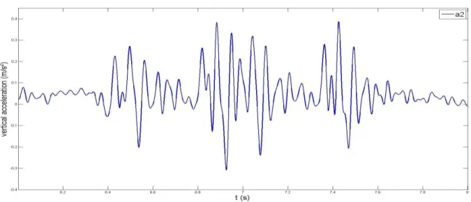
For these different meshes vertical deflection, vertical acceleration and stresses in the crown and springline of the pipe beneath the track centre were analysed. The time history of mesh number five is shown in Figure 3.7. See also appendix A.2.

Figure 3.7: Crown results for mesh number five in 3D. a) vertical crown deflection, b) vertical crown acceleration, c) crown bending moment and d) crown normal force.

Table 3.7 shows the maximum values for deflection, acceleration and section forces in the crown.

Table 3.7: Maximum values for deflection, acceleration and section forces in the crown for 3D meshing.

Mesh

nr. [mm] dmax [m/samax 2_] _[kN/m]Nmax _[kNm/m]Mmax

1 0,4273 0,7726 7,89 0,0385

2 0,4301 0,8113 8,97 0,0439

3 0,4303 0,8109 9,04 0,0433

4 0,4338 0,8530 9,03 0,0450

(50)

32

Figure 3.8 shows the quotas of deflection, acceleration and section forces in the crown generated using the five different meshes as compared with mesh number five. The quotas are shown in the figure as a function of the average element size, see Table 3.6.

Figure 3.8: Quotas of max deflection, acceleration and section forces in the crown for the five different meshes, as compared with mesh number five.

Mesh number five was used for the dynamic calculation presented in section 4.1.2.

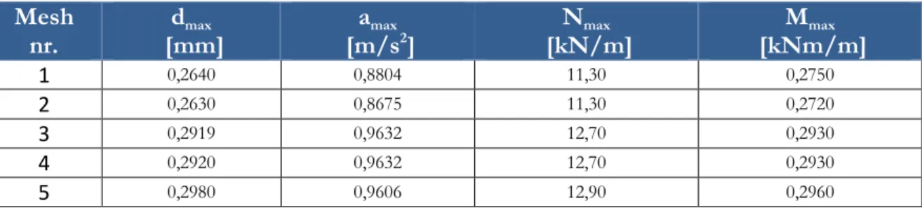
3.7.2 2D

In the 2D mesh, 15-node triangular elements have been chosen for the soil material. The plates consist of line elements, which are 5-node when combined with the 15-node triangular elements which are used for the soil, as described in sections 5.6.4, 5.6.6 and 7.1 of [18]. The interface elements are attached to the sides of the 15-node triangular soil elements and consist of five pairs of nodes.

In the mesh tab, the “Generate mesh” button opens the mesh options dialogue. Using expert settings allows for insertion of relative element size, re. The relative element size

governs the average element size, le, according to Formula 3.2 shown below.

√( ) ( ) 3.2

In section 7.1.1 of [18], re and nc seem to be used interchangeably. There are five

options available in Plaxis for element distribution if expert settings are not used. These are listed below.

 Very coarse – correlates to re equal to 2,0  Coarse – correlates to re equal to 1,33  Medium – correlates to re equal to 1,0

(51)

33  Fine – correlates to re equal to 0,67  Very fine – correlates to re equal to 0,5

The default setting for meshing in Plaxis is “Medium”, i.e. re equal to 1,0. As in the 3D

meshing, a fineness factor (note that [18] refers to this factor as fineness factor whereas it is named coarseness factor in the 2D software itself) can be chosen for each geometric entity. The default value is 1,0 for all geometric entities except for structural components and loads, which have a fineness factor of 0,25.

Five different mesh qualities were used in order to find a suitable mesh for the 3D model. Table 3.8 shows the specifics of each mesh.

Table 3.8: Mesh properties, 2D.

Mesh properties, 2D

Mesh nr. Entity Fineness _factor

1

Boundary lines 0,25

Number of elements 8884 Sleepers -

Ballast 0,25 _{Number of nodes} ₇₂₀₄₅ Backfill 0,5

Pipe 0,125

Average element size [m] 0,1591 Relative element size 0,6

2 Boundary lines 0,25 Number of elements 11151 Sleepers - Ballast 0,25 Number of nodes 90243 Backfill 0,5

Pipe 0,125 _{Average element size [m]} _0,1420 Relative element size 0,5

3 Boundary lines 0,25 Number of elements 15882 Sleepers - Ballast 0,25 Number of nodes 128393 Backfill 0,5 Pipe 0,125

4

Boundary lines 0,25 _{Number of elements} ₂₁₀₆₀ Sleepers -

Ballast 0,25

Number of nodes 170105 Backfill 0,3536

Pipe 0,08839

5

Boundary lines 0,25 _{Number of elements} ₃₆₁₆₄ Sleepers -

Ballast 0,1768 _{Number of nodes} ₂₉₁₃₈₅ Backfill 0,25

Pipe 0,06250

Dynamic analysis of soil-steel composite railway bridges: FE-modeling in Plaxis

Dynamic analysis of soil-steel

composite railway bridges

FE-MODELING IN PLAXIS

Dynamic analysis of soil-steel

composite railway bridges

FE-modeling in Plaxis

O

ROD

A

AGAH

S

IAVASH

A

RYANNEJAD

Master of Science Thesis

Stockholm, Sweden 2014

Abstract

Sammanfattning

Preface

Contents

List of Figures

List of Tables

1

Introduction

1.1 Soil-steel composite bridges

1.2 Design and dynamics

1.3 Previous studies

1.4 Aim and scope

1.5 Structure of the thesis

2

The soil-steel composite bridge in

Märsta

2.1 Bridge location and traffic

2.2 Bridge specifications

2.3 Instrumentation and measurement

3

FE- modelling in Plaxis

3.1 About Plaxis

3.2 Model properties

3.3 Creating soil layers

3.3.1 Soil materials

3.3.2 Boreholes

3.4 Creating plates and beams

3.4.1 Creating plates in 3D

ν),

ν).

3.4.2 Creating beams in 3D

3.4.3 Creating plates in 2D

3.5 Creating interfaces

3.6 Creating point loads and load multipliers

3.6.1 3D

3.6.2 2D

3.7 Mesh

3.7.1 3D

3.7.2 2D