2017:11 Extended Common Load Model: A tool for dependent failure modelling in highly redundant structures

(1)

Research

Extended Common Load Model:

A tool for dependent failure modelling

in highly redundant structures

2017:11

(2)

(3)

SSM perspective

Background

The treatment of dependent failures is one of the most controversial subjects in reliability and risk analyses. The difficulties are specially underlined in the case of highly redundant systems, when the number of redundant components or trains exceeds four. The Common Load Model (CLM), originally defined in the 70’ies, differs from other CCF models, as it relies on a specific physical analogy. The model was extended in late 80’ies with specific aims to model highly redundant systems. Practical use of the model requires a computer tool, but in highly redundant systems the benefits give an evident payback.

Objectives

The extended method ECLM details have not been publicly available before. However, it has been developed with certain funding via the Nordic PSA group (NPSAG) including SSM. It has therefore been an interest to have the method properly documented and published. The objective with this report is to describe the mathematical details in the definition of Extended CLM (ECLM), which is developed to better suit for modelling of highly redundant systems. ECLM has four parameters, while the initial CLM was a two-parameter model. This report focuses on parameter definition and interface between a dedicated CCF analy-sis and PSA models. The estimation of model parameters is described for Maximum Likelihood and Bayesian approaches. Also a comparison is presented with respect to other common CCF models. Special exten-sions are described for time-dependent modelling and asymmetric CCF groups.

Results

The result is that the method is documented and available for the stakeholders, including SSM. The report is also published as an NPSAG report.

Need for further research

There is no continuation planned for this since it is the end result of previous work.

Project information

Contact person SSM: Per Hellström Reference: NPSAG Project no. 34-002

(4)

(5)

2017:11

Author: Tuomas Mankamo

Avaplan Oy, Esbo, Finland

Extended Common Load Model:

A tool for dependent failure modelling

in highly redundant structures

(6)

This report concerns a study which has been conducted for the Swedish Radiation Safety Authority, SSM. The conclusions and view-points presented in the report are those of the author/authors and

(7)

Summary

This report describes an extension of Common Load Model, specially developed for the treatment of failure probabilities and dependencies in highly redundant systems. The model is based on expressing failure condition by stress-resistance analogy; at the demand, the components are loaded by a common stress, and their failure is described by component resistances. A multiple failure occurs, when the load exceeds several component resistances. In Extended Common Load Model the load constitutes of base and extreme load parts, modelling failures at low and high orders, respectively. Four parameters are defined; for each part a probability parameter describing likelihood level and a correlation coefficient describing failure dependence. Good or reasonable fit has been obtained with dependence profiles in failure statistics even for large component groups. The estimation of model parameters can be based on standard procedures of maximum likelihood method or Bayesian method.

The model is defined in terms of subgroup failure probabilities and is subgroup invariant. This implies that the model applies with same parameter values to any subgroup of a homogeneous group, so called Common Cause Failure group. Subgroup invariance facilitated application of the model is varying demand conditions where different parts of the group are challenged. Furthermore, model parameters applicable to two separate groups of different size are directly

comparable, if mutually homogeneous or under assumption of that, which is helpful also in data acquisition.

ECLM is basically defined as pure demand failure probability model. It can be extended to other types of failure on demand like instantaneous unavailability of standby components and failure over mission time. Further extensions have been made during the course of applications to model access criticality and failure correlation of adjacent control rods, and asymmetric groups like in case of design diversification, e.g. redundant components of old and new, and partially same design.

The main limitation is generally sparse statistical data about Common Cause Failures, a shared problem of parametric models for Common Cause Failures. The problem is pronounced with the model extensions where additional features should be verified by operational experience; much is based on engineering judgment for the time being.

Applications of ECLM concentrate in the Nordic BWR plants, for safety/relief valve systems, and control rods and drives. These applications have been

supported by the collection of Common Cause Failure data for analysed systems. Applications to control rods and drives have been made also in French PWR plants. Other applications include highly redundant configurations of isolation valves and check valves, and main steam relief valves of a Russian RBMK plant.

(8)

Acknowledgements

The comments and support by the PSA team of Teollisuuden Voima Oy are acknowledged in the course of the initial development of the presented method and procedures for practical applications. The presentation of methodology has benefited from the comments by Aura Voicu, EdF in the connection to local applications. The valuable review comments by Sven Erick Alm, Uppsala University, and Christine Bell, AREVA NP GmbH, are also taken into account, especially aiding to improve the description of parameter definition. Jan-Erik Holmberg, Risk Pilot AB has greatly helped by advices and comments in the finalizing stage of this document.

Notice

Extended Common Load Model is implemented in HiDep Toolbox, developed by Avaplan Oy, containing various tools for the quantification of Common Cause Failures in different types of highly redundant systems. HiDep rights are now transferred to the following members of Nordic PSA Group: Forsmark

Kraftgrupp AB, OKG AB, Ringhals AB and Teollisuuden Voima Oy which have also supported the elaboration of this document. Risk Pilot AB will maintain HiDep software and provide future user support. Generic HiDep Toolbox version is available to professional users under open software terms, contact

(9)

1 Introduction

1.1 Characteristics of the CCF analysis for highly redundant systems

The treatment of dependent failures is one of the most controversial subjects in the reliability and risk analyses [CCF_PG, NKA/RAS-470]. The difficulties are specially underlined in the case of highly redundant systems, when the number of redundant components or trains exceeds four. The Common Load Model (CLM), originally defined in [CLM_77], differs from the other CCF models, as it relies on a specific physical analogy. This proves to be advantageous in several respects as will be explained in the continuation, and when comparing with the other approaches. The model was extended in late 80’ies with specific aims to model highly redundant systems. Practical use of the model requires a computer tool, but in highly redundant systems the benefits give an evident payback.

The motivation to this development arose from the practical needs to realistically assess the failure probability of the overpressure protection and pressure relief function in the PSA study at Teollisuuden Voima Oy (TVO). The TVO/BWR units (Olkiluoto 1 and 2) had twelve safety/relief valves (SRVs) at that time before modernization. The SRVs are imposed on demand in different ways depending on the transient case and event scenario. The success criteria range from 4/8 to 1..9/12. This early application has been described in [SRE88HiD]. TVO/PRA included also early applications to other highly redundant systems, including control rod and drive system.

1.2 Scope of this report

This report describes the mathematical details in the definition of Extended CLM (ECLM), which is developed to better suit for modelling of highly redundant systems. ECLM has four parameters, while the initial CLM was a two-parameter model. This report focuses on parameter definition and interface between a dedicated CCF analysis and PSA models. The estimation of model parameters is described for Maximum Likelihood and Bayesian approaches. Also a comparison is presented with respect to other common CCF models. Special extensions are described for time-dependent modelling and asymmetric CCF groups.

1.3 Applications

Since the early applications to TVO/PRA the following works can be highlighted:  Analysis of SRV experience was carried out incorporating Swedish BWR

units, and a reference application prepared for Forsmark 1/2, emphasis given on the integration with PSA models [SKI TR-91:6].

(12)

 CCF analysis of the hydraulic scram and control rod systems, including the analysis of operating experiences of the Nordic BWRs and reference application to Barsebäck 1 and 2 [SKI-R-96:77]

 Development of a time-dependent extension for risk monitor or follow-up purpose and test arrangement analysis of highly redundant systems

[TVO_SRVX]

 Quantification of asymmetric system configurations for SRVs (for the modernized TVO plant and a new plant concept) and for containment isolation valves

Similar new applications have been made more recently for other plants, including following cases:

 Control rods and drives in French PWR plants [ICDE-EdF-2001]

 Highly redundant configurations of isolation valves and check valves, and main steam relief valves of Leningrad plant (RBMK).

Earlier applications have been upgraded, especially for control rods and drives [SKI Report 2006:05].

The practical applications have implied gradual development of the calculation tools. The treatment of critical failure combinations of control rods and drives has been enhanced for increased realism. Basic definition of ECLM has stayed as initial during the course of time and different kinds of applications.

(13)

2 Basic Concepts

To begin from, it is important to clearly specify, what is the measure of failure probability which is then primarily used to express dependencies among a group of components called as CCF group – or in the current terminology Common Cause Component Group (CCCG). The treatment of the subject is focused here to the quantification of time-independent failure probabilities or so called demand failure probabilities of standby components. A time-dependent extension of ECLM is discussed in Section 7.2.

2.1 CCF group and subgroup concept

Identical components of a CCF group, normally in standby, are imposed in the model, to an operation demand. The event of basic interest is the failure of specific ‘m’ components in the demand. The probability of such an event is denoted by

Psg(m) = P{Specific m components fail|Demand on CCF group n} (2.1) Particular variable notation “Psg” for Probability of SubGroup failure is used here, in order to make a clear distinction with respect to often confused probability notations.

The CCF group will be assumed internally homogeneous, hence Psg(m) is same for any choice of ‘m’ components, which constitute a subgroup of the considered CCF group. It is also assumed, that if the demand is placed only on a part of components, the failure probability of any challenged ‘m’ components will be same in the challenged subgroup, e.g. no extra stresses are imposed if fewer components participate in the system response. Such influences should be

modelled separately. Especially, the total component failure probability Psg(1) is equal among the components, and remains same in different demand conditions. This aspect should not be confused with the treatment of event combinations which differ depending on the applicable failure criterion for the demand condition (to be discussed in Chapter 4).

An example of a highly redundant CCF group of ten electromagnetic pilot valves (EPVs) is presented in Figure 2-1. In a depressurization demand, a subgroup of eight EPVs are actuated to open the corresponding SRV main valves (which form a different CCF group). Four lines are sufficient to achieve the required fast pressure reduction. Consequently, if a subgroup of five or more EPVs fail within the challenged subgroup of eight EPVs, depressurization fails. An additional aspect influencing subgroup under focus is a situation where DC power supply to EPVs is degraded. For example, if one of the DC buses is down for maintenance (8 hour’s Allowed Outage Time in power state applies at the Olkiluoto 1 and 2 plant), the depressurization function needs to be accomplished by a subgroup of six EPVs. The failure criterion changes from nominal 5 out of 8 into 3 out of 6.

(14)

An example of the critical failure combination when DC bus A is inoperable, and of the corresponding failure probability is:

Psg(3) = P{XEPV181 * X EPV182 * X EPV184 } (2.2)

where XEPV# denotes the failure of a specific EPV, compare to Figure 2-1. It should be emphasized, that the probability Psg(3) does not take into account the status of other 7 EPVs: they may operate or fail at demand, or may not be challenged at all if power or actuation signal is missing. Chapter 4 will explain, how the total failure probability of system function is derived from the basic probability entities Psg(m), which are preferred in the ECLM definition.

(15)

Figure 2-1 Illustration of a subgroup of size 8 in a CCF group comprising n=10 identical

components for Olkiluoto 1 and 2 depressurization function (configuration before the plant modernization in 90’ies). In the depressurization demand 8 SRV lines are challenged: those SRV lines are presented by solid boxes, while the other two (which participate only in overpressure protection) are presented by dashed boxes. V02..13 denote main valves and EPV179..188 denote electromagnetic pilots. The success criterion is 4 out of 8 in this example, i.e. failure events of multiplicity 5 are minimal cut sets. The SRVs are equipped also with diverse impulse pilot valves that are spring-operated and provide backup actuation in overpressure protection. The impulse pilot valves are not part of remotely actuated depressurization function and are hence not presented in this simplified diagram.

V11 - EPV186 V13 - EPV188 V06 - EPV181 V10 - EPV185 V02 - EPV179 V07 - EPV182 V08 - EPV183 V09 - EPV184 V12 - EPV187 V03 - EPV180 Sub A Sub B Sub C Sub D 4/8

(16)

Similarly, as for BWR reactor relief system, the success criteria vary for many safety systems depending on the initiating event and successful operation or failure of other systems. These different demand and success criteria cases need to be handled consistently. For this reason, it is beneficial, that the CCF

quantification model applies to subgroups within the system with the same model parameters. This property is called subgroup invariance. It will be discussed in more detail in Chapter 4, along with its practical implications. The above defined Psg(m) entities are an example of subgroup invariant variables under the assumed conditions of internal symmetry within the CCF group. Consequently, the size of the whole CCF group need not be explicitly denoted as part of the variable

notation for Psg entity in the case that it is evident from the context what is meant by the subgroups. In the connections where the size of the whole CCF group is needed to be emphasized, notation Psg(m|n) can be used. Compare to further discussion of the different probability entities in Chapter 4.

Probability Psg(m) is monotonously decreasing for increasing failure multiplicity. The term dependence profile will be used to mean the shape of Psg-curve,

especially related to how failure probability is saturating at high orders.

2.2 Stress-resistance expression

In the CLM, the failure condition is expressed by stress-resistance analogy: at the demand, the components are loaded by a common stress S, and their failure is described by component resistances (strengths) Ri, compare to Figure 2-2 and Eq.(2.3.a). Both the common stress and component resistances are assumed stochastic, distributed variables. A multiple failure occurs, when the load exceeds several component resistances, compare to Eq.(2.3.b) presented as part of

Figure 2-2.

In this model, the dependence arises partly from the common load, partly from the identical resistance distributions of the components. However, within the resistance distribution, a component may individually vary from the others. The actual resistances are not exactly known prior to the demand, which effectively places the components in symmetric position (assumption of homogeneity). A relatively wide distribution of resistances means low dependence in general, because then it is less likely that a particular load exceeds several components’ resistances at the same. The opposite condition of relatively narrow distribution of resistances means high dependence, because then it is likely that if the load exceeds the resistance of one component the same can happen for several other components also. The properties of the inherent dependence mechanism in CLM are discussed more thoroughly in the original introduction to the model

[CLM_77].

The probabilities Psg(m) are the measurable entities: a specific multiple failure profile can evidently be produced by many different choices of the stress and resistance distributions. The normal distributions are still used in the extension

(17)

multiplicity. In the extension, there are four parameters which are defined and discussed in more detail in Chapter 3 and Appendix 1. Nevertheless, only four parameters prove to describe adequately dependencies in highly redundant, internally homogeneous groups as far as statistical data are available. STRESS-RESISTANCE EXPRESSION

S > Ri for each i in a specific subgroup of m components (2.3.a) SUBGROUP FAILURE PROBABILITY EXPRESSION







    x m R S(x .)F (x) f. dx ) n | m ( Psg (2.3.b) where

fS(x) = Probability density function of the common stress

FR(x) = Cumulative probability distribution of the component

resistances

Figure 2-2 Basic concepts in the Extended Common Load Model (ECLM).

RESISTANCES Strengths of the identical components F_R(x_Ri) Stress/Resistance Variables Pro ba bility Den sity or D is tr ibut ion Total load Base load Extreme load STRESS Common load f_S(x_S) Random x_S Random selection of x_Ri

(18)

2.3 Practical interpretation of the model

The general stress-resistance expression (2.3) can be refined to describe common and independent failure causes for each component in the following way

sc + si > rc + ri (2.4)

where

s_{c = Common stress imposed to all components}

s_i = Independent stress fluctuations from component to component r_{c = Common or nominal resistance of the components}

ri = Resistance variations from component to component Each of these two common entities and 2*n component specific entities are stochastic variables. Assuming the components are identical and form a

homogenous CCF group, the si have identical distribution and ri respectively. The expression can be rearranged by moving common entities on the left and

component specific entities on the right hand side:

i i i c c R S s r r s     _ ___   (2.5) Comparing this reduced form to the general stress-resistance inequality (2.3) reveals that the "generalized" common load S comprises those failure mechanism factors that increase common part of stress or decrease common part of

resistance. Similarly, the "generalized" resistances Ri comprise those factors which increase individual part of the resistances or decrease individual part of the stresses.

The above discussion applies to a CCF group which is internally symmetric. In case of asymmetry, the stress/resistance variables can be arranged

correspondingly, which provides a basis to further extensions of the approach. If there would be available sufficient knowledge about the failure mechanisms, and statistical distributions for the contributing factors, the analysis could be made "explicitly" at the level of inequality (2.4). In case of some simple structural elements this might be possible in practice. In most cases there exist too large a number of potentially significant failure mechanisms, each too rare to obtain statistical data. Then it is motivated to apply the stress-resistance inequality in its reduced form (2.2), and use some suitable distributions with convenient

parametrization. The distributions are fitted to the measurable probability entities Psg(m), in order to estimate the distribution parameters or the equivalent model parameters.

(19)

3 Parametrization of ECLM

Due to the way of definition, ECLM is a very general model. The same

probability pattern of multiple failures can be obtained (at least with reasonable accuracy) by using many alternative distributions for common load and

component resistances. For practical uses it is essential to adopt parametric distributions, which are both well understandable in practical terms, and mathematically convenient to apply.

3.1 The use of normal distributions

In the early definition, normal distributions were used, and simple

parametrization with just two parameters, total component failure probability and correlation coefficient, were found suitable for low redundant cases [CLM_77]. In highly redundant cases this proved not sufficient to describe observed

probability patterns of multiple failures, i.e. fit to empirical values of Psg(m). Several alternative ways of extension were explored, including the use of extreme value distributions for common load. The trial and error phase resulted in the most suitable option, where load distribution was extended to the superposition of two normal distributions, base and extreme load parts:

fS(x) = wSb.fSb(x) + wSx.fSx(x) , (3.1)

where wSb and wSx are weight fractions (positive numbers which sum up to 1). The resistance distribution was retained as sole normal distribution.

Correspondingly, the integration equation, Eq.(2.3.b) divides up into base load and extreme load parts:









) m ( Psg ) m ( Psg ) x ( F .) x ( f. dx . w ) x ( F .) x ( f. dx . w ) m ( Psg xtr bas x m R Sx Sx x m R Sb Sb    



      (3.2)

The key idea in the extension is targeting the base load part to describe failure probabilities at low multiplicities, and the extreme load part to the (often stronger) dependence at high multiplicities.

The normal distribution is not only convenient to use, but it can be expected to be rather generally valid as in most cases the failure mechanisms are random

processes with large number of contributing terms. If the contributions influence additively, normal distribution often applies. On the other hand, if the most significant variables contribute multiplicatively, then lognormal distribution often applies, or alternatively stated, logarithmic transformation brings the situation back to the additive case. The lognormal and normal distributions are fully

(20)

compatible to be used for underlying distributions of CLM, as shown in detail in [CLM_77].

In the superposition above, the extreme load part can be interpreted to describe environmental shocks, latent design faults, systematic maintenance errors or combinations of these which may cause a large number of identical components to fail concurrently. Basically, further parts can be added to the load distribution. However, two parts have been up to now sufficient to fit with empirically

observed probability patterns of multiple failures (in homogeneous groups). The fit has been in fact surprisingly good even for higher order failures in many cases when statistics have been available. Experiences from model fit to failure data are discussed further in Chapter 5. Specific kinds of further extensions have been made in non-homogeneous cases to model internal asymmetry of component group, to be discussed later.

3.2 Choice of model parameters

In the extension, the following four model parameters are defined:

Table 3.1 Parameters of the Extended Common Load Model, range in practical

applications.

Parameter Description Range Typical value

p_tot Total component failure

probability [0, 0.5] 10

-4_{- 10}-2

p_xtr Extreme load part as contribution to the single failure probability

[0, p_tot] p_xtr/p_tot  1% … 5%

and p_xtr >10-5

c_co Correlation coefficient of the

base load part [0, c_cx] 0.1 … 0.5

c_cx Correlation coefficient of the

extreme load part [c_co, 1] 0.6 … 0.9

Mathematical details of the parametrization will be handled in Appendix 1. To summarize, the distributions are scaled as (0, dSb)-normal for base load, (1 - dR,

dSx)-normal for extreme load and (1, dR)-normal for resistance. The probability

parameters are related to Psg(1) and correlation coefficients to standard deviations {dSb,dSx,dR} in the following manner:

 

₂ R 2 Sx 2 Sx xtr 2 R 2 Sb 2 Sb d d d cx _ c ; 1 Psg xtr _ p d d d co _ c ; 1 Psg tot _ p       (3.3)

(21)

The parameters form two pairs. The first pair {p_tot, c_co} is related to base load part, and the other pair {p_xtr, c_cx} to extreme load part. The adopted

parametrization yields in reduced coupling between the pairs, giving the benefit of intuitively clear impact of the parameters on the multiple failures: pair {p_tot, c_co} describes the probability level and dependence at low multiplicity and pair {p_xtr, c_cx} correspondingly at high multiplicity.

The existence of three underlying distributions {fSb,fSx,fR} means in total 6

distribution parameters. Because a linear translation of the stress/resistance variable does not affect the failure probability Psg(k), the degrees of freedom is effectively 5. In the chosen parametrization, one degree of freedom is frozen by anchoring the relative position of fSx at a specific point between medians of fSb

and fR, i.e. leaving only the variance of fSx free. (Base load median is set at 0,

extreme load median at 1, and resistance median at 1 - dR, compare to the details

in Appendix 1.) This specific anchoring gives the desired reduced coupling between parameter pairs {p_tot, c_co} and {p_xtr, c_cx}.

It must be emphasized that certain weak coupling is imposed by adopting total component failure probability p_tot as one model parameter. This is due to following relationship, compare to Eqs.(3.2-3):

p_tot = p_bas + p_xtr, where p_bas = PsgBas(1) (3.4) Especially, it is good to be aware that in a sensitivity analysis where, for example, p_xtr is varied while keeping other parameters constant (p_tot also constant) base load part adapts in opposite direction compared to p_xtr. Even though the

reflected changes in base load part are small they show up clearly in dependence profile in a way that looks strange if one is not aware of the underlying

relationship. The influences become simpler and more intuitive by keeping p_bas as constant when varying dependence parameters p_xtr, c_co and c_cx, i.e. allow p_tot floating.

The optional choice of parameter pairs {p_bas, c_co} and {p_xtr, c_cx} as model parameters would be mathematically convenient. But from practical point of view p_bas has to be replaced by p_tot. It should be noticed that p_bas is usually numerically very close to p_tot.

A further coupling is imposed by using dR in the definition of both c_co and c_cx

in order to obtain unified normalization, see Eq.(3.3). These relationships will be discussed in more detail in Appendix 1, Section 8, including advices for the parameter variations in sensitivity analyses.

It needs to be also emphasized that parameters c_co and p_xtr interfere because they contribute in parallel to low order failures. This interference will be

(22)

Usually p_xtr lies at or above the level of 10-5 or near to a few percent relative to p_tot, compare to Table 3.1. Mathematically p_tot is limited in ECLM below 0.5 due to the fixed relative placement of distributions. In practice total component failure probability is well below that limit. The correlation coefficients have values between [0, 1]. The value 0 means total independence and value 1 total dependence. Practically meaningful relationship is c_cx  c_co. Often the base load correlation lies in the range of 10%..50%, while the typical value of the extreme load correlation is in the range of 60%..90%.

It should be noted that the parameters defined for the ECLM above, are related to the output of the model rather than to the stress and resistance distributions directly. Only the total component failure probability can be estimated in direct way from the number of failures per number of test/demand cycles. The other parameter estimates cannot be expressed in closed form but must be solved using Maximum Likelihood search or Bayesian method, and computerized estimation tool. The details of estimation will be handled in Chapter 5.

3.3 Subgroup invariance

With the given model parameters, numerical integration of the stress-resistance expression produces probability values for multiple failures, primarily for Psg(m). From the Psg entities then other types of probability entities can be derived following the transformation scheme to be discussed in Chapter 4.

Due to this scheme, ECLM fulfils the subgroup invariance requirement, which is evident also from the definition of the model. This means first of all, that the same model parameters apply in each subgroup, which is very convenient for practical uses. On the other hand, the parameters of CCF groups with different size are directly comparable. This enhances much the utilization of information from analogical cases - without a need to manipulate the event data from different sizes of CCF groups by use of complex mapping up/down methods. Compare to the further discussion of this aspect in [NAFCS-PR03].

(23)

4 Calculation of Failure Probabilities

One of the central innovations in this integral approach to the treatment of dependencies in highly redundant structures is the consideration of various kinds of probability entities for subgroup failure, each providing a different point of view. Acronym SGFP is used here for subgroup failure probability.

4.1 Subgroup failure probability concepts

As stated in Chapter 2, we are considering a CCF group of n identical components. The basic entity is the failure probability a specific set of

components defined in Eq.(2.1). It will again be emphasized that this entity has following invariance properties in internally homogeneous CCF group (of n components):

Psg(k|m) = Psg(k|n) = Psg(k), for any k  m  n, and (4.1) for any selection of k and m components

Subgroup of m components can denote a demand subgroup or any other embedded CCF group to be considered for analysis aims.

Subgroup invariance means that, for example, the probability of k specific

components failing is same whether they are considered alone or as a subgroup of the total n components, in both cases, disregarding the information on the other's survival or failure, i.e. Psg(k|k) = Psg(k|n) = Psg(k).

The failure dependencies are in ECLM primarily modelled via Psg entities and numerically derived from integration Eq.(2.3.b). The other (structural) probability entities are then constructed in the following way.

Assuming the demand is imposed on m components, the success criterion can be interpreted also via the equivalent failure criterion k out of m. The associated total failure probability of the reliability structure is denoted by (notation “Pts” comes from total for the structure):

Pts(k|m) = P{k or more out of m components fail | Demand on

subgroup m } (4.2)

For example, in case of Figure 2-1, the failure criterion is 5 out of 8, and Pts(5|8) is the desired result value.

There is an exact one-to-one correspondence between Pts(k|m) and Psg entities, but Pts(k|m) is not subgroup invariant by any means, instead it is directly coupled to the demand group size m and failure criterion k out of m. The transformations

(24)

are presented in Figure 4-1 (notice that the equations there are derived for a demand group of size n, but they apply equally well to any subgroup m  n, when n is a homogeneous CCF group). The algorithms are based on standard

probability calculus and their derivation is discussed in [SKI TR-91:6].

Figure 4-1 Transformation scheme of subgroup failure probability entities in a

homogeneous CCF group of n components. These algorithms apply also within any subgroup of the whole CCF group.

Pts(k|n) = P{ Some k or more out of n

components fail }







Pes(k|n) = P{ Exactly some k out of n

components fail, while the other n-k survive }

TR3'

Psg(k|n) = P{ Specific k components

fail in a CCF group of n }

Peg(k|n) = P{ Just the specific k out of n

components fail, while the other n-k survive } TR1 TR1' TR3 TR2 TR2' ) n | k ( Peg . ) n | k ( Pes : TR2 k n        ) n | k ( Pes . 1 ) n | k ( Peg : TR2' k n       



          n k m ) n | m ( Peg ) n | k ( Psg : TR1 . k m k n

 



            n k m ) n | m ( Psg ) n | k ( Peg : TR1' . k m k n . k m 1

Transformation scheme

(25)

The transformations can conveniently be made by the use of the exclusive subgroup failure probabilities by (notation “Peg” comes from exclusive for the group):

Peg(k|m) = P{Just the specific k out of m components fail, while the other m-k survive|Demand on subgroup m } (4.3) In some context it is convenient to include the number of combinations of k out of m, into this exclusive probability concept yielding a related entity by (notation “Pes” comes from exclusive for some):

Pes(k|m) = P{Just some k out of m components fail, while the

other m-k survive|Demand on subgroup m } (4.4) If written out, the transformation equations become quite long in case of, for example m=10. But computationally they do not present any big problem as the required code fragments become short when applying usual recursive technique. In conclusion, Psg entity has a key position among the four different SGFP entities, basically owing to its subgroup invariance. The great benefit of using Psg entity, for example in data comparison, is the fact that it describes the dependence profile of the increasing failure multiplicity without “disturbance” of

combinatorics and order exclusion which affect the other SGFP entities. On the other hand, the three other SGFP entities have each a specific area of use in modelling and quantification of dependencies.

4.2 Calculation of SGFPs by the use of ECLM, EPV example

To summarize what was said in the preceding section, the usual flow of calculations is following:

ECLM(Parameters:= p_tot, p_xtr, c_co, c_cx)

→ Psg(k) → Peg(k|m) → Pes(k|m) → Pts(k|m) (4.5) The calculation order needs to be changed in ultra-high redundant systems

because of numerical accuracy limitations with Psg(k) → Peg(k|m)

transformation in large groups as will be discussed in Chapter 6. The above calculation order is used in so called ‘base’ implementation with scope of groups up to 20 … 30 components, depending on ECLM parameter values.

Using the EPV example of Figure 2-1, the result of ECLM integration are first presented in Figure 4-2 and then the SGFP entities are derived for different subgroups in Figure 4-3. Details related to the parameter estimation will be discussed later in Chapter 5. Concerning the demand group of 8 EPVs challenged in a depressurization need, the desired result is Pts(5|8) for failure criterion 5 out of 8.

(26)

The example shows a usual dependence profile. Values of Psg(k) saturate quite strongly at higher multiplicity, as the extreme load part Psgxtr becomes then

dominating, while the base load part Psgbas is determining at low multiplicities.

Due to the strong dependence at higher multiplicities, the Peg(k|m) values become rather small at intermediate multiplicities for bigger subgroups, which is also quite usual.

Figure 4-2 Probability quantifications by the use of ECLM for the CCF group of ten

EPVs for Olkiluoto 1 and 2 [RESS_HiD]. HiDep Version 2.1

Extended Common Load Model Avaplan Oy, March 1997

TVO 1/2, electromagnetic pilot valves, best estimate

Point estimate CCF group size CLM parameters ND 34

KmMax 10 p_tot 4.0E-2 c_co 0.40 VfSum 12.95 p_xtr 3.0E-3 c_cx 0.80 p_est 3.81E-2 Km Psg_b Psg_x Psg Zk Peg Pes Pts Vk Sk/ND

0 0.991 9.03E-3 1.000 - 0.775 0.775 1.000 26.50 1.000 1 3.70E-2 3.00E-3 4.00E-2 0.040 1.38E-2 1.38E-1 2.25E-1 5.00 2.21E-1 2 6.04E-3 2.15E-3 8.19E-3 0.205 1.04E-3 4.69E-2 8.73E-2 1.00 7.35E-2 3 1.78E-3 1.77E-3 3.55E-3 0.434 1.66E-4 2.00E-2 4.04E-2 0.80 4.41E-2 4 7.15E-4 1.55E-3 2.26E-3 0.637 4.49E-5 9.43E-3 2.04E-2 0.50 2.06E-2 5 3.47E-4 1.40E-3 1.74E-3 0.770 1.87E-5 4.71E-3 1.10E-2 5.88E-3 6 1.92E-4 1.28E-3 1.47E-3 0.846 1.17E-5 2.45E-3 6.29E-3 5.88E-3 7 1.16E-4 1.20E-3 1.31E-3 0.890 1.11E-5 1.34E-3 3.84E-3 0.15 5.88E-3 8 7.47E-5 1.13E-3 1.20E-3 0.915 1.81E-5 8.12E-4 2.50E-3 1.47E-3 9 5.09E-5 1.07E-3 1.12E-3 0.932 6.37E-5 6.37E-4 1.69E-3 1.47E-3 10 3.61E-5 1.02E-3 1.06E-3 0.943 1.06E-3 1.06E-3 1.06E-3 0.05 1.47E-3

LogLikeL -21.313 DeltaLL 0.000 1E-6 1E-5 1E-4 1E-3 1E-2 1E-1 1E+0 1 2 3 4 5 6 7 8 9 10 11 12 Failure multiplicity Fa ilure proba bility Psg_b Psg_x Psg Peg Pes Pts Sk/ND

(27)

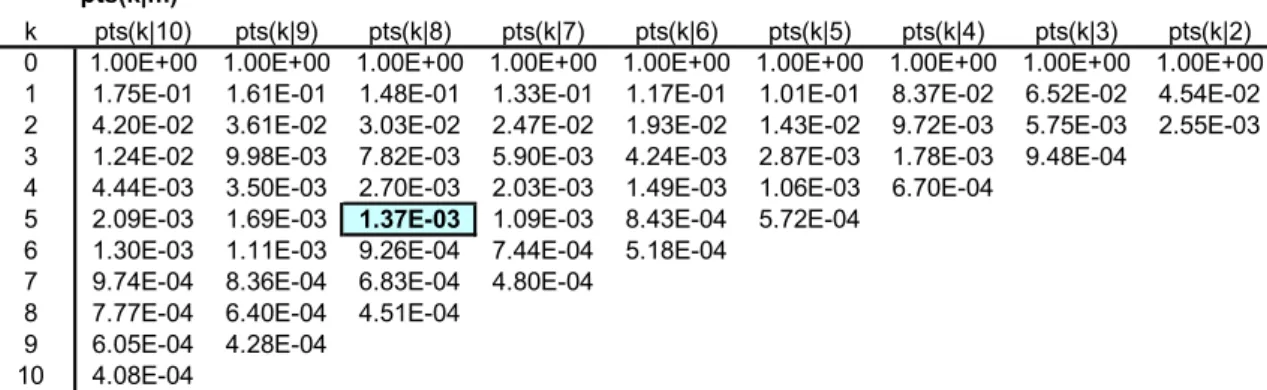
Figure 4-3 Generated failure probabilities for any subgroup of the ten EPVs for

Olkiluoto 1 and 2 [SKI TR-91:6].

pts(k|m)

4 4.44E-03 3.50E-03 2.70E-03 2.03E-03 1.49E-03 1.06E-03 6.70E-04 5 2.09E-03 1.69E-03 1.37E-03 1.09E-03 8.43E-04 5.72E-04

6 1.30E-03 1.11E-03 9.26E-04 7.44E-04 5.18E-04 7 9.74E-04 8.36E-04 6.83E-04 4.80E-04

8 7.77E-04 6.40E-04 4.51E-04 9 6.05E-04 4.28E-04

10 4.08E-04

TVO I-II Electromagnetic pilot valves/FO best estimate

psg(k) 1.0E-6 1.0E-5 1.0E-4 1.0E-3 1.0E-2 1.0E-1 1.0E+0 1 2 3 4 5 6 7 8 9 10 11 12 Failure Multiplicity k Fa ilu re P ro ba bi lit y pts(k|m) pts(5|8) peg(k|m)

(28)

4.3 Interface to PSA models

In standard PSA approach, the CCF basic events are used as an interface to PSA fault trees. This frame becomes increasingly tedious to use due to rapidly

escalating number of event combinations for CCF groups of five or more components. Instead, the dominant contributors can be expressed by a limited number of appropriately defined functional events and by using SGFP entities. For example, in Olkiluoto 1 and 2 PRA (initial design), only 11 interface entities were used for the SRVs as compared to about 210_*22_*212_{component event} combinations between electromagnetic pilots, pneumatic pilots and main valves within 12 SRV modules (10 ordinary safety/relief lines and 2 regulating relief lines).

It should be emphasized, that the definition of interfacing events needs to be done carefully, in order to properly take into account risk-significant cross

combinations with loss of activation signals, failure of power buses and other hardware or functional dependencies. Experiences this far show that a rather limited number of these cross combinations are important, which implies that the interface from a highly redundant CCF group can be managed.

As an example, the interface with electric power supply dependence can often be most conveniently structured according to the failure situations of power buses. For example, in the case of depressurization demand, when 8 SRV lines are challenged, and with failure criterion 5 out of 8, the EPVs contribute effectively in the following schematic way (compare to Figure 2-1):

PtsEff(5|8)  PtsEPV(5|8) + 4 . uDCB . PtsEPV(3|6) (4.6)

where

uDCB = Mean fractional downtime of a DC bus supplying EPVs

This is a usual Rare Event Approximation: the first term corresponds to the situation where the four DC buses are all available, but five or more of the EPVs fail; the second term corresponds to the situation where one DC bus is down for maintenance, and in conjunction three or more of the six EPVs fail in the other subs. In practice, there may exist other cross-combination terms, which need to be included in a similar way [SKI TR-91:6]. The identified terms can then be

transformed into equivalent functional event presentation to be incorporated in the system fault trees.

4.4 Comparison with the approaches based on the structure of common cause events

The mostly used CCF models Multiple Greek Letter Method (MGLM) and Alfa Factor Method (AFM) are based on describing dependencies by the use of CCF basic events. Normally, CCF basic events with input probabilities Q , are

(29)

explicitly included in PSA fault tree models, and MCS reduction is cared by a computer program. This provides a very convenient interface into PSA models, which works well in low redundancy cases. In high redundancy cases, due to the large number of CCF basic events to be added for many component gates, MCS reduction becomes overwhelmingly burdened. Hence, the pre-processed, reduced presentation in terms of functional events and SGFPs for the PSA model interface as described in the preceding section is the preferred approach.

In practice, if AFM/MGLM would be used, a reduction into the SGFP scheme is the only viable way in highly redundant cases. The problem is that the SGFPs cannot be expressed exactly in terms of the CCF basic events. In low order cases, relatively simple approximations exist, but in high redundancy cases, handling of combinatorics and necessary approximations become cumbersome. Besides, the AFM/MGLM parameters are not subgroup invariant (an example about the parameter variability is presented in [SKI TR-91:6]). This means that cases, where only part of the system is challenged, become laborious to handle. One way is to consider the subgroup as imbedded in the whole group, preserving all CCF basic events for the total group, selecting those which validate the failure criterion in the subgroup demand case. This has been the usual way. Alternative way is to map AFM/MGLM parameters and CCF event probabilities down to the CCF group corresponding with the demanded subgroup. This necessitates the use of rather complicated routines. In contrast, when a subgroup invariant model is used, the same CCF parameters apply to any subgroup.

(30)

5 Parameter Estimation

Due to the lack of a reverse analytic solution for the stress-resistance analogy expression, a formula-based direct estimation of ECLM parameters is impossible (except for one parameter, the total component failure probability p_tot). Hence, standard numerical methods for Maximum Likelihood search or Bayesian estimation have to be applied. It should be noticed that most other parametric CCF models, when used in highly redundant cases, necessitate also the use of computerized estimation tools.

5.1 Likelihood Function

The Likelihood Function can be constructed in the usual way given the available information about success/failure events in a group of n components over a number of test/demand events [Henley&Kumamoto]:



  n 0 k ) n | k ( V )] n | k ( peg [ )}) n | k ( V { | cx _ c , co _ c , xtr _ p , tot _ p ( Lik (5.1) where

V(k|n) = the number of failure events of multiplicity k in a CCF group of n components, i.e. Sum Impact Vector

V(0|n) = the number of success events, i.e. test/demand cycles in which all components survived

ND = the number of tests and demands on the whole group of n components



  n 0 k V(k|n)

An example of Sum Impact Vector V(k|n) is given in the subtable of Figure 4-2; its derivation from operating experience is explained in [SKI TR-91:6].

Constructing the Sum Impact Vector from the failure records follows the general principles presented in [CCF_PG]. Compare also to the more recent method description [NAFCS-PR03]. A refined approach is developed in an application, which uses state model to describe the development of latent CCF mechanisms and chances to detect them in random demands between test points [T314_TrC]. For the calculation of the Likelihood Function, Peg(k|n) entities are obtained from Psg(k) entities, using the transformation presented in Figure 4-1, while Psg(k) values have first been integrated from the stress-resistance analogy expression, Eq.(2.3.b) - with distribution parameters derived from the model parameters. The whole scheme of the estimation cycle is illustrated in Figure 5-1. As described in Chapter 3 the model parameters are intentionally chosen to

(31)

outcome of the model. In the background the model parameters are

mathematically connected to the stress/strength distributions. The benefit of this parametrization approach is that the behaviour of the model outcome is well predictable with respect to the parameters.

Figure 5-1 Flow scheme of parameter estimation for ECLM.

The drawback is, as said, that the model parameters cannot be directly calculated from the count of failure events. The indirect estimation is required for ECLM. The compatibility verification for the fit of model with the empirical failure pattern will be discussed in more detail in Section 5.3.

Example shapes of the Likelihood Function, with respect to the model parameters p_xtr, c_co and c_cx, are presented in Figure 5-2. The example case is the same as used earlier, the group of ten EPVs in Olkiluoto 1 and 2. Compare to the point estimation in Figure 4-2.

An apparent benefit of Likelihood Function-based approach is that it allows a convenient scheme for combining event data from different sources and from CCF groups of different sizes (which assumes a mutual homogeneity, or a

postulation of that as an approximation, see further details of CCF data pooling in [NAFCS-PR03]). In the first approximation, joining data bases A and B results in the following compound Likelihood Function, corresponding to weighting by the total number of test/demand cycles (the Sum Impact Vector without elements is denoted by bold capital letter V):

) .( Lik *) .( Lik ) , .( Lik_A_&_B V_A V_B  _A V_A _B V_B (5.2) Compa-tibility ECLM Estimation method Event information Impact vectors_V

i(k|n) S(k|n)/ND

ECLM parameter set M =

{p_tot, p_xtr, c_co, c_cx} Pts(k|n)



  n k m ) n | m ( V ) n | k ( S

(32)

Compound Likelihood Function can be used also in the case of asymmetric tests or demands to combine statistical data over test/demand subgroups.

Figure 5-2 Illustration of the Likelihood Function behaviour for p_xtr, c_co and c_cx

separately at the maximum [ECLM-Tcases]. The example case is the ten EPVs of Olkiluoto 1 and 2 [RESS_HiD].

5.2 Total component failure probability

The point estimate for the total component failure probability p_tot can be obtained from the total number of failures:

where , ND n ) n ( VfSum tot _ p   (5.3) failures of number total the ) n | k ( V k ) n ( VfSum n 1 k is



   -0.20 -0.10 0.00 0.10 0 0.1 0.2 0.3 0.4 0.5 0.6 0.7 0.8 0.9 1 Correlation Coefficients c_co, c_cx

Relat ive Dif fe rence of Log10(Lik(.

)) _{Base Load: c_co}

ExtremeLoad: c_cx

-0.20 -0.10 0.00 0.10

0.0E+0 2.0E-3 4.0E-3 6.0E-3 8.0E-3 1.0E-2 1.2E-2

Extreme Load Part p_xtr

Relative Differenc

(33)

5.3 Comparison with empirical failure pattern

The evidence and the model can best be compared by constructing the empirical failure pattern:

S(k|n) = Number of test/demand events where k or more out of n components are failed





 n

k

m V(m|n) (5.4)

Dividing this by the total number of tests/demands ND gives the point estimate of the total structural failure probability, i.e.(look for this kind of comparison in Figure 4-2): ND ) n k ( S ) n k ( Pts  (5.5)

For comparison purposes, this relationship is preferred due to the stable nature of S(k|n) profile even in the case of sparse data. However, the comparison could alternatively be performed between SGFPs and their point estimates:



                  n k m _mn k m k n ND ) n | m ( V ) k ( Psg (5.6)

5.4 Maximum likelihood search strategy

The Likelihood Function appears to be rather smooth and searching the maximum point can be simplest done by interactively controlled numerical iteration. The point estimate for the total component failure probability p_tot, obtained from Eq.(5.3), can be kept constant during the search process.

The search for the other model parameters can be started from usual values. If no other clue is readily available, the following initial values can be used:

p_xtr ~ 0.03*p_tot (5.7)

c_co ~ 0.4 c_cx ~ 0.8

Practical experiences show, that it is preferable to first search after a reasonable fit of the extreme load part p_xtr, because the dependence pattern is most

(34)

iteration round can be based on visual comparison of Pts(k|n) and S(k|n)/ND fit as explained above, compare also to Figure 4-2. Fine tuning can then be performed by considering numerical changes of Likelihood Function. The current version of HiDep Toolbox contains a semi-automated tool for the search of the maximum likelihood estimates.

Because of the stable nature of Likelihood Function, and because the model parameters influence largely independently to outcome probabilities, the maximum likelihood search converges soon for the adopted ECLM parametrization. In most cases less than ten trials are sufficient in order to identify p_xtr, c_co and c_cx all with a reasonable accuracy. The particular details of the parametrization, which broke the dependence between the pairs {p_tot,c_co} and {p_xtr,c_cx} prove thus useful. The model parameters can nevertheless interfere in estimation. For example, c_co and p_xtr can contribute in parallel to low order failures, implying a diagonal correlation in Likelihood Function. The surface determined by Likelihood Function can rise in a direction deviating from c_co and p_xtr coordinate directions. This aspect can be

controlled by watching Likelihood Function values for a grid of parameter values, or by using some developed search algorithm for the maximum of a

multi-parameter function.

In case of sparse data for high multiplicity failures, extreme load part p_xtr can be considered primary parameter for the dependence at high multiplicity, while extreme load correlation c_cx has a side role, and can be preserved at the typical value of 80%.

For correlation coefficients c_co and c_cx, the Likelihood Function is usually rather symmetric on the linear scale, and the maximum point is apparent, Figure 5-2. The width of the maximum area may be quite broad (absolute value of the second derivative small) if data are sparse.

For the extreme load part p_xtr, it is more natural to consider the Likelihood Function on the logarithmic scale for p_xtr: it is usually rather flat towards small values, but decreases steeply for higher values when approaching the area which contradicts with the evidence about the number of high multiplicity failures, or if p_tot will be approach. If data are sparse, there may not be a maximum point at all for p_xtr, but the Likelihood Function may be monotonously (although weakly) increasing for decreasing p_xtr. If this happens to be the case, the Bayesian estimation approach is to be preferred. In the absence of Bayesian estimation tool, the following shortcut can be used: p_xtr should be chosen at the level where the Likelihood Function begins to significantly reduce from the plain level at smaller values of p_xtr.

5.5 Experiences from parameter estimation

(35)

mechanical and electrical parts, component boundary, and operational, test and maintenance environment, as well as similarity in defenses against CCFs.

Some data compilations contain CCF data pooled over much different component types, e.g. pooled data of all demand failures. Such data represent a statistical mixture of failure mechanisms and CCF types which can be problematic to apply to a specific target component. It is hence recommended to find out reference data for earlier analyzed similar component type.

A possible last resort is the use of parameters of so called Generic Dependence Classes, see discussion in [Nafcs-PR02, Section 4.2]. They were originally derived for CCF groups of size up to four, covering component types like pumps, valves, breakers and diesel generators. So they may not be applicable in highly redundant systems.

The statistical input (Impact Vector) can in some cases contain a large number of complete CCFs. This can mean that no sensible parameter estimates are obtained, e.g. maximum likelihood is obtained at null correlation coefficients. This

situation can be related to mapping up of complete CCFs observed in smaller component groups, which may be unrealistic conservative. The dilemma of mapping up has been discussed in [NAFCS-PR03, Section 6.2]. Possibly, actual complete CCFs can have actually occurred due to some specific causes in the size of CCF group under consideration. Exceptionally large number of complete CCFs is most likely related to special CCF mechanisms like external events or other events beyond normally defined component boundary, or systematic operational, test or maintenance errors or system design errors, or combination of these. A possible solution is to separate special complete CCFs and model them explicitly, and cover the other part of statistical data by parametric CCF model.

Another peculiar Impact Vector is such a case where the elements are strongly decreasing as the function of multiplicity. This situation can arise, for example, if binomial model is used to map up potential CCFs, compare to the discussion in [NAFC-PR03, Section 6.2]. Maximum of Likelihood Function can be then

obtained with null extreme load part. The statistical significance of Impact Vector is in such a case anyhow weak at high orders. Generic data can be used for

extreme load part parameters. Leaving extreme load part out reduces ECLM to the early defined two parameter CLM. Experiences thus far show that in all cases with sufficient statistics the dependence profile of real components contains an outstanding extreme load part.

In some cases, the statistical input can show peculiarities caused by

inhomogeneity. For example, exceptionally many failures of order two may have occurred in a group of four components due to weaker defence against CCFs between redundancy pairs, i.e. the group is pair-wise asymmetric. A

recommended solution is to divide CCFs to those possible for the whole group and those specific to redundancy pairs, resulting in smaller CCF subgroups to be modelled in addition to the whole group.

(36)

CCF model comparison [CCFCoFin] contained estimation tests with a large number of different data sets. This material can provide useful insights for the elaboration of new data cases.

5.6 Model behaviour as the function of ECLM parameters

Inherited from the definition, the model parameters have the following meaningful ranges for practical application:

0.5 > p_tot > p_xtr > 0 (5.8)

0 < c_co < c_cx < 1

Looking for the visual "look and feel", it should be emphasized once more, that the parameters form two pairs. The probability parameters p_tot, p_xtr give the value wherefrom the associated Psg-curves start at multiplicity k=1. The

correlation coefficients c_co, c_cx describe the slopes of the curves: small value means weaker dependence and steeper decrease of the probability as the function of failure multiplicity, while a value of c_cx near to 1 would result in strong saturation at higher failure multiplicities.

As a specific feature of this approach, it should be noted that the CLM inherently allows individual variation in component vulnerability to failure, as described by the resistance distribution. As a benefit, this model will not show so strong tendency of producing overly pessimistic dependence at high multiplicity in case of sparse data, as most other models, which often reduce effectively to a

conservative "cut-off" probability at high failure multiplicities.

5.7 Bayesian estimation outline

Besides maximum likelihood search, the Likelihood Function serves as a basis for the more developed Bayesian estimation. This approach will be shortly outlined here as related to beginning experiments used to estimate Pts(k|n). According to the standard Bayesian approach, the expected value of model related Pts(k|n) can be obtained from:



pts(kn)



dp .dc .dc f. (p ,c ,c .)pts(kn;p ,c ,c )

E 

_

_x _o _x _Post _x _o _x _x _o _x (5.9)

where the normalized, compound posterior density function is



 ) c , c , p ( Lik .) c ( f ). c ( f ). p ( f. dc . dc . dp ) c , c , p ( Lik .) c ( f ). c ( f ). p ( f ) c , c , p ( f x o x x cx _ c o co _ c x xtr _ p x o x x o x x cx _ c o co _ c x xtr _ p x o x Post V _V

(37)

Here, the total component failure probability p_tot is considered fixed (but the scheme could be readily extended to handle it as the fourth free parameter). Apriori distributions are noted as fp_xtr, fc_co, fc_cx for the other three model parameters considered free variables in the estimation. For the Likelihood

Function, a shorthand notation is used here as compared with Eq.(5.1). Similarly, the notation for parameters p_xtr, c_co, c_cx are shortened to px, co, cx.

For the apriori distributions, the simple piecewise linear- constant shapes are used as shown in Figure 5-3, considering p_xtr on the logarithmic scale and correlation coefficients c_co, c_cx on the linear scale. The distribution shapes reflect the judgment about the

 possible range of parameters (nonzero distribution density)  most likely range (constant distribution density)

The derived expected values are noted on Figure 5-3. They prove to be in quite a good agreement with the maximum likelihood values, assuming a reasonable amount of data. The behaviour of Likelihood Function for c_cx is not shown here, it is very flat, compare to Figure 5-2. The expected value of c_cx is thus determined in the example case by the a priori distribution. Even generally, the a-priori distributions have a big role and their choice is therefore crucial in

(38)

Figure 5-3 Illustration of the behaviour of Likelihood Function, and a priori distributions

and posterior distribution of Pts(5|8) in Bayesian estimation experiments in 1990. E[c_co]=0.36 0 0.2 0.4 0.6 0.8 1 ‐21.7 ‐21.6 ‐21.5 ‐21.4 ‐21.3 ‐21.2 0.0 0.2 0.4 0.6 0.8 1.0 Ap rio ri, N on ‐N or m al ize d Log 10 o f L ik el ih oo d Fu nc tio n c_co, c_cx Log10 LF c_co prior c_cx prior E[p_xtr]=2.5E‐3 0 0.2 0.4 0.6 0.8 1 ‐21.7 ‐21.6 ‐21.5 ‐21.4 ‐21.3 ‐21.2

1.00E‐5 1.00E‐4 1.00E‐3 1.00E‐2 1.00E‐1

Ap riori , N on ‐N orm al ize d Log 10 o f L ik el ih oo d Fu nc tio n p_xtr Log10 LF p_xtr prior 5%: 9.5E‐4 50%: 4.7E‐3 Mean: 5.9E‐3 95%: 1.3E‐2 0% 10% 20% 30% 40% 50% 60% 70% 80% 90% 100%

1.E‐4 1.E‐3 1.E‐2 1.E‐1

Cu m ul at iv e D ist ributi on Pts(5|8)

(39)

5.8 Uncertainty treatment

The uncertainties and their treatment in the CCF analysis of highly redundant systems is similar to probabilistic safety analyses in general. The sparse data on high multiplicity failures mean that the uncertainty range is large. Engineering judgment is often used extensively in the interpretation and extrapolation of the data. A special difficulty is concerned with how to take into account design changes or other countermeasures which are usually implemented after CCF occurrences. The verification of the learning effect is a difficult issue.

The uncertainty impact on the results and conclusions of the analysis can be in the simplest approach be investigated by sensitivity analyses/parameter

variations. A more consistent evaluation of uncertainties can be made by Bayesian approach which is straightforward to apply in case of ECLM, representing a well-behaving, ordinary parametric model.

Advanced techniques are recently developed in France for ECLM parameter estimation [PEstim-ECLM-FR2013].

(40)

6 Ultra High Redundant Systems

This chapter handles application of ECLM to ultra-high redundant systems like control rods and drives extending the methodology description presented earlier in [SKI Report 2006:05] and recent application reports.

Special care is required for numerical accuracy in the calculation of multiple failure probability at the orders with very high number of component

combinations as will be discussed in Section 6.1.

In the case of control rods and drives an additional specific aspect is important. The failures of adjacent control rods impose much bigger reactivity effect in comparison to spread failure placements. This aspect concerns failure

consequences but does not violate the assumption about homogeneity of CCF group. The treatment of adjacent rod patterns in the definition of failure criteria will be discussed in Section 6.2.

Some CCF mechanisms are more likely in the case of adjacent control rods and drives, representing a special type of non-homogeneity of CCF group. These so called localized failure mechanisms are considered in Section 6.4. Main part of CCF mechanisms can be regarded to have no position correlation, i.e. control rod and drives can be modelled as a homogeneous CCF group with respect to them. These so called scattered failure mechanisms are considered in Section 6.3, covering also the general case of ultra large homogeneous CCF group. Section 6.5 combines the calculated results over different failure mechanisms.

The failure probabilities are considered in this chapter as so called demand failure probabilities.

6.1 Arrangement of probability calculations in very large groups

The calculations in very large CCF groups have to be arranged so that Peg entity is derived first from the following version of ECLM expression, compare to analogous Eq.(2.3) used to obtain Psg entity:

��|�� _�� �� ∙ �� ∙ ��∙ �� (6.1)

This route is necessary to avoid problems with small differences in Psg entity values and very large binomial coefficients at the intermediate multiplicities in a very large group, implying that transformation Psg(Km) → Peg(Km|KmMax) containing alternative positive/negative terms cannot be handled with a standard double accuracy of computer programs in ultra-high redundant cases. However, the opposite transformation Peg(Km|KmMax) → Psg(Km) contains only positive terms, and is manageable up to CCF group sizes of at least about 160, a practical limit in the applications to control rods and drives of Nordic BWRs.

(41)

Alternatively, Psg and Peg entities can be integrated in parallel. The

transformations Peg(Km|KmMax) → Pes(Km|KmMax) → Pts(Km|KmMax), needed to find out the failure probability of the system function for a given failure criterion, deal only with positive terms, and is manageable also in ultra-high redundant cases.

An implication of the above feature is that scale down to a subgroup cannot be performed based on a subset of Psg(Km) similarly as in the base implementation of ECLM, using the subgroup invariance property of Psg entity, compare to earlier discussion in Section 3.3. In ultra-high redundant case the subgroup system needs to be re-quantified in order to obtain Peg entity within the

subgroup, which effectively means a change of the CCF group size (KmMax), a drawback of ‘ultra’ implementation. Scale down needs are fortunately not frequent in ultra-high redundant systems whereas they are typical in CCF modelling of safety/relief valves and similar systems.

It has to be noticed that there is no low bound for using ultra-implementation (with the sacrifice that probability entities of subgroups cannot be derived without complete recalculation). Thus ultra-implementation can be applied to a group of twelve safety/relief valves, for example, to verify the results with respect to using base implementation for the same group (with same data).

6.2 Failure criteria for control rods and drives

The placement of control rods with respect to horizontal cross-section of reactor core can be described by so called control rod map where X and Y coordinates are given to each control rod. A selection of control rods can be denoted by the following different ways:

 Group, especially when meaning physical components

 Combination or set, typically in the treatment of failure events  Pattern in the control rod map, like in Figure 6-1

Group size refers to the number of included control rods. Term shape is used for geometrical type of control rod pattern.

The third dimension, coordinate Z describes the degree of insertion. Usually it is expressed by the degree of withdrawal: fully inserted as Z = 0% and completely withdrawn as Z = 100%. This dimension is not usually taken into account in risk analysis. In normal operation part of control rods is completely withdrawn, part partially inserted. It is conservatively assumed that all control rods are completely withdrawn before demand. Furthermore, partial failure of insertion (stagnation at an intermediate position) is not covered among the modelled failure modes, only complete failure of insertion. The treatment of complex phenomena in failure event analysis and classification is discussed in more detail in the recent data analysis [SKI Report 2006:05].