The (in)efficiency of Financial Markets : Applying the Relative Strength Strategy on the Swedish Large cap Exchange

(1)

The (in)efficiency of Financial Markets

Applying the Relative Strength Strategy on the Swedish Large cap Exchange

Bachelor Thesis in Economics Department of Business, Society & Engineering

Mälardalen University Author: Rickard Varli

Supervisor: Christos Papahristodoulou Spring 2021

(2)

Abstract

This paper examines the efficiency of the Swedish stock market, specifically the Large cap list of the Stockholm stock exchange. This is achieved by implementing the relative strength method of investing during the decade of 2010-2020 and evaluate the results in contrast to the Efficient Market Hypothesis. The relative strength method applied in this paper is the similar strategy that Jagadeesh & Titman (1993) utilized. In short, the strategy is based on buying the historically best performing stocks whilst selling short the previous worst performers. Additionally, the risks associated with the method were examined with the risk measurements of the Jensen Alpha and the Modigliani risk-adjusted performance. The results indicate that the relative strength method is unable to consistently generate above-market returns, so that the study is unable to reject the Efficient Market Hypothesis. In addition, the relative strength method is unable to justify the risks associated.

Acknowledgement

I would like to thank my supervisor Christos Papahristodoulou for his valuable feedback and ideas during the time of the study. His knowledge was enormously helpful to improve the quality of the work.

(3)

1.Introduction

The first chapter of the study introduces the core of financial markets and subsequently the research problem. Thereafter, the chapter concluded by stating the aim of the study and the research question.

1.1 Background

Financial markets provide corporations with valuable methods of financing. Corporations with financial needs are able to sell stock to certain investors. In return for the risk, investors may be able to sell the stock or collect dividend payments. However, certain events affected the financial markets severely, these rare occurrences are events such as “Tulip Mania” and “Dot-com boom.”

Therefore, investors and academics such as Jagadeesh & Titman (1993), asked themselves the question of whether financial markets are efficient?

This important question has been investigated significantly over the years with different perceptions. The basic idea of the research is to primarily test the efficiency of the markets by attempting to generate above-market returns. Therefore, investors and academics have constantly tried to find profitable investment strategies that are able to generate excessive and consistent returns thus, to beat the market.

1.2 Problem Discussion

Since the Efficient Market Hypothesis (EMH) was developed by Fama (1970), it serves as the most fundamental and influential tool in financial theory. The Efficient Market Hypothesis is characterized by expressing that the prices of various assets and securities fully reflect all available information that is

fundamental to its price. This implies that no investment strategy of any kind, or investor with great, or not so great intelligence will be able to generate above-market returns, with an equal risk exposure.

Although, the Efficient Market Hypothesis is essential in the area of finance, it is also a subject of debate and received various reactions. Malkiel (2003) argues that daily prices for stocks and other assets deviate randomly, based on the flow of information that is disclosed. Since information occurs randomly and is

unpredictable to investors, then the resulting price changes are also unpredictable and random. The research of Malkiel (2003) agrees with the random walk theory

(6)

6

and with the EMH but is also mentioning that predictable patterns and pricing irregularities will appear as a result of irrational market participants.

Others, such as Jung & Shiller (2006) support the Efficient Market Hypothesis when it is intended for individual securities as any given stock but opposes it when analyzing macroeconomic market dynamics. The reason is that the new information occurs more frequently for individual corporations compared to the economy as a whole. In other words, there is typically more frequent information, such as earnings rapports and other fundamental qualities for individual

corporations, rather than macroeconomic information.

There have also been various proposals where historical data and information regarding stocks and other securities can be able, along with a variety of methods to create portfolios that generate above-market returns. De Bondt & Thaler (1985), French & Roll (1986), Jagadeesh & Titman (1993), Dreman & Barry (1995), Rouwenhorst (1997), George &. Hwang (2004) and Parmler & Gonzalez (2007) have all found market anomalies by using various strategies. Furthermore, the researchers used their various ideas and strategies to generate above-market returns. The findings of these various studies should not be achievable if the Efficient market Hypothesis is truly valid.

Since, Rouwenhorst (1997) and Parmler & Gonzalez (2007) found different results when investigating the Swedish stock market, although with different sample periods, it is appealing to further study this topic. Thus, the efficiency of the Swedish stock market will be investigated in this study.

1.3 Aim

The purpose of the study is to examine whether the Swedish stock market is efficient as the EMH states.

In order to fulfill the purpose of the study, this paper will pursue to answer the research question of:

(7)

7

2. Review of Literature

The second chapter of the study starts with explaining the three levels of market efficiency, followed by the random walk hypothesis. Thereafter, the chapter is concluded by previous studies that disagree with the Efficient Market Hypothesis.

2.1 The Efficient Market Hypothesis

The theory of efficient markets became widely adopted when Fama (1970) developed the theory, which stated that asset prices, at any given period will reflect all current information on the market. If markets The EMH presumes that all information is equally distributed and transparent to both buyers and sellers and therefore, the price fluctuations should be unpredictable to forecast for both parties. Consequently, if the Efficient Market Hypothesis is correct, it is

impossible for an investor to obtain above-market returns without accepting above-market risk. The theory makes the assumptions that, all participants interpret information, prices, and the future distribution of prices similarly. The Efficient Market Hypothesis states three forms of market efficiency and is briefly described as (Fama, 1970):

I Weak-form efficiency

The weak-form of market efficiency describes that asset prices reflect and mirror all previous information that exists. Furthermore, if markets are thought to act weak-form efficiently, it implies that there is no correlation among historical and future prices. Hence, any investment method based on historical prices in order to predict future prices will fail. In other words, one cannot predict the market based on any reappearing pattern or behavior.

II Semi-strong efficiency

The semi-strong form of market efficiency is a more radical version of the EMH and suggests that asset prices reflect all publicly available information, as well as historical information. This means that financial statements, unemployment figures, or any other information that may be essential to value an asset is equally available for all other investors. When new information about a security arises, the price will adjust to a new equilibrium based on the mutual interpretation of the shareholders. Hence, no other investor will be able to create abnormal returns using public information.

(8)

8 III Strong-form efficiency

Finally, the third and final form of market efficiency is the strong-form of market efficiency. This suggests that asset prices reflect all accessible information. The strong form of market efficiency also includes private

information that yet to arrive at the market. Thus, this implies that no investor, not even one with insider information will be able to create abnormal returns. It is notable that insiders such as CEOs and board members is required to follow strict regulations when purchasing stocks.

Hence, the EMH believes that any excess returns generated

relative to the market derive either from luck or randomness. This was investigated by Malkiel (2019), where he compared passive versus active managed funds. The concept of passive funds was to track the overall market, with relatively low fees and inversely, the actively managed intended to beat the market by using knowledge and expertise, that enables them to charge higher fees. The findings were that actively managed funds were unable to beat the passively managed ones, and therefore also underperform relative to the market portfolio. The conclusion of Malkiel (2019) is in support of the EMH, and states that the market portfolio, given equal risks will outperform any other form of investment. Keown & Pinkerton (1981) constructed an event study which aimed to test the semi-strong form of market efficiency. In order to do this, the authors examined a sample of corporations that were targets of takeover attempts. Consequently, the stock of these firms would dramatically increase since the acquiring company would pay a premium. However, the stock of the firms did not further vary and drift, but rather found an equilibrium which Keown & Pinkerton (1981)

interpreted as support to the EMH since the market responded to the new public information instantaneous.

However, Grossman & Stiglitz (1980), question the possibility of perfect information, as expressed by the EMH. If all investors are able to acquire information and thus, is reflected in the prices of assets, why would anyone then gather information? Subsequently, there would be no incentive for individuals to

Figure 1. Illustration of the EMH. Source: Bodie, Kane & Marcus (2010

(9)

9

acquire information. Furthermore, there would be little incentive to trade various assets and commodities in the market. Consequently, financial markets would have been of very little use in society. Furthermore, Shiller (2016) argues that the EMH is accountable for several “bubbles” and overinflated prices, which

inevitably will crash. The reason is that the EMH states that any market price for a security is correctly priced at the market.

2.1.1 The Random Walk Theory

The Random Walk theory is closely related to the Efficient Market Hypothesis and to some extent, the outcome of it. The random walk theory emphasizes that changes in asset prices are truly independent and suggests that price movements are comparable to dice rolls or coin flips (Brealey, 2019). As a result of

unpredictable asset movements, the only factor able to determine a certain stock price over time is randomness. Consequently, it should be unachievable to find predictable market anomalies. This suggests that the methodology certain

academics use, where investigating historical price movements will fail to predict future price movement.

Worthington & Higgs (2004) tested the random walk theory in several European stock markets. Their hypothesis was to investigate the presence (or absence) of serial correlation in the financial markets, where serial correlation implies how well the historical price of a security predicts the future price and. The researchers conclude that the Swedish stock market fulfill the strictest random walk criteria. This implies, according to Worthington & Higgs (2004) that the Swedish stock market is weak-form efficient.

The outcome of the random walk theory is that stocks do not follow regular price cycles as one might expect, but rather independent and random events. Similarly, if price movements for stocks followed a well-defined pattern, then the correlation of the daily returns would be positive. However, according to Brealey (2019) this turns to be very close to zero. Hence, the prices and trends for the previous day provides no effect for future prices. Consequently, as demonstrated by Malkiel (2019), plotting random outcomes of coin flips in a chart, and comparing it to a fictional security gives rather similar results.

(10)

10

2.2 Previous Research on Relative Strength

The relative strength investment method buys and sells various securities based on their historical returns. This investment method is believed to generate above-market returns as demonstrated by the researchers below, who argue that the market a non-random walk.

De Bondt & Thaler (1985) examined the efficiency of the US stock market and found rather interesting anomalies. By the term anomaly, De Bondt & Thaler (1985) suggests that the general theory and assumptions of the EMH, which were tested and fails in practice. This was done during the years of 1926-1982 by collecting monthly sample data from the US stock market. The researchers examined stocks that had risen and fallen in value steeply.

The hypothesis of De Bondt & Thaler (1985) was that stocks that had over- or underperformed relative to the market, would reverse. This is also known as the mean-reversion effect where the basic concept is that stocks that deviate, either positively or negatively from their mean, will reverse to their equilibrium. The findings of De Bondt & Thaler (1985) were that stocks that previously have underperformed relative to the market earns about 25 percent more than the stocks that have previously overperformed against the market. De Bondt & Thaler (1985) also argue that the larger the overreaction the stocks experience, the bigger the correction will be. In other words, if a certain stock significantly overperformed relative to the market, then they will also experience a rather significant price drop.

Jagadeesh & Titman (1993) apply the relative strength strategy equivalently as De Bondt & Thaler (1985). They did though have the opposite approach, the idea of Jagadeesh & Titman (1993) was stocks, which historically overperformed will continue to overperfom in the future. Meanwhile, the opposite would occur for those stocks that underperformed. Another distinction between the two studies is that Jagadeesh & Titman (1993) examined shorter time-horizons than De Bondt & Thaler (1985).

Jagadeesh & Titman (1993) managed to generate above-market returns for all porfolios constructed. In particular, the strategy generated consistent above-market returns that varied anywhere between 1,31 percent per month to 0.32

(11)

11

percent per month. All returns generated were statistically significant and in addition, they also demonstrated that their results were not a consequence of excessive risks, viewed as the β-value for respective portfolio. The relative strenght strategy have been implementend by others, such as Moskowitz & Grinblatt (1999) and Rouwenhorst (1997) with a few variations.

Moskowitz & Grinblatt (1999) constructed a study with the idea of buying and selling stocks in various sectors and industries. The thought was that certain sectors and industries would over and underperform relative to the market. This was due to over- and underreactions by investors given any event such as earnings reports. The similar idea was also shared by Keynes (1936), who considered that business cycles occur, as a cause of fluctuations from investor profit expectations. The authors, then bought the three highest performing sectors and sold the three worst performing sectors and form equal weighted portfolios. This was done during the years of 1963-1995 in US stock markets.

Their findings show a positive relationship between past and future returns during intermediate time-horizons, similar to the results of as Jagadeesh & Titman (1993). While also finding reversal effects during shorter (≤ 1 month) and longer time periods (3-5 years), similarly as De Bondt & Thaler (1985).

Analogous studies have been conducted in European stock markets. Rouwenhorst (1997) examined the method on several stock markets. During the years of 1978-1995, the author examined monthly returns for stock market corporations in twelve different European countries. Rouwenhorst (1997) finds significant profits in eleven European stock markets while the Swedish stock market was the only market that could not prove excess return on a statistical significance level. However, some years after Parmler & Gonzalez (2007) managed to find

profitability in the Swedish stock market by using the relative strength method. By using the relative strength method of investment, these various studies found above-market returns. This, according to the authors contradicts the theory of efficient markets. However, Malkiel (2003), criticize the legitimacy of researchers who claim that various anomalies discovered inevitably disprove the Efficient Market Hypothesis. Malkiel (2003) argues that these studies are solely dependent on a specific sample period and therefore, lack robustness. For instance, the

(12)

12

hypothesis of given researcher might work exceptionally well during certain market conditions, or otherwise fail.

Malkiel (2003) also emphasizes that any strategy that is thought to be profitable will self-destruct. The author argues that, the more potentially profitable a pattern is the less likely it is to survive. The reason is simply that investors do not “leave any $100-bills on the ground.” Better explained, investors will outbid each other until no profitability further exists. Hence, any repetitive pattern or strategy that exploits the market fundamentals will be exploited by investors until it ceases to exist. However, Shiller (2016), argues that any kind of investment method, or speculation that disregard fundamentals and asset pricing theory, will inevitably create asset prices that deviate from realism.

3. Methodology

Chapter three will initially explain the methodical approach, and the statistical tools used. Furthermore, the risk measurements used in the study will be explained. Thereafter, the collection of data, process, calculations, and various selections will be explained. At last, the chapter is concluded by describing the limitations and eventual difficulties of the study.

3.1 Methodical Approach

By using the approach of Jagadeesh & Titman (1993) this study aims to buy the stocks that previously overperformed during J-months and sell stocks that

underperformed during the same period. Similarly, as Jagadeesh & Titman (1993) the assets will be bought and sold short into equally weighted portfolios and held during K-periods. Furthermore, the strategy is perceived as successful if it is able to, as Jagadeesh & Titman (1993) generate above-market returns consistently. The returns of the strategy will be compared to the benchmark selected. Additionally, the risks of the portfolios will be examined by using the measurements of the Jensen Alpha and also the Modigliani risk-adjusted

performance, the reason that these two measures are used is due to that risk often differently defined.

A security may be labeled as a winner or loser depending on the preferred time-horizon of the investor. Thus, the formation period (J) implies the time-time-horizon where the security is analyzed and segmented into the P10 (winner) portfolio, the

(13)

13

P1 (loser) portfolio, or else disregarded because of mediocre returns. The holding period (K) denotes the months that the asset is held by the investor.

The various JK-months implemented in the study will be 3-, 6- , 9- and

12-months. This implies that the portfolios will be constructed by the previous 3-, 6-, 9- and 12-months returns, while also being held for the following 3-, 6-, 9- and 12-months.

Furthermore, this means that the identical stocks for each J-month period will be held for all K-months. For instance, the best and worst performing stocks during the J3 period will be held for K3, K6, K9 and K12, where it is concluded. The identical process follows for all remaining JK-month portfolios. This also implies that the same stock may be traded for several portfolios and years, depending on its previous performance. For instance, if a certain stock performed poorly during several years, then it could be sold during those years.

To enhance the legitimacy of the study, the portfolios will be formed with overlapping holding periods. For instance, the same J12K3 portfolio discussed above, that holds the assets for three months will be overlapped by the J12K6 portfolio that consists of the identical assets, but with a holding period of six months. Thereafter, the identical overlap will occur by the remaining K9 and K12 portfolios, until all portfolios are summarized. The identical method will be implemented for all of the JK portfolios such as the J3 strategy displayed below. The portfolios will afterwards be evaluated for the given year and subsequently continue for the following years.

Figure 2. Illustration of the structure of the J3K3 investment strategy for a given year. There is a possibility that for example, any buy portfolio will generate profit whilst the sell portfolio generates negative yield. Thus, it is possible that either portfolio will over- or underachieve equally, which may produce zero-sum return. Therefore, in accordance with the study of Jagadeesh & Titman (1993) the

Month

1 2 3 4 5 6 7 8 9 10 11 12 +1 +2 +3

Formation Period Holding Period

(14)

14

analysis will consist of three phases where they evaluate the results of the buy portfolio, that consists of buying the best performers. The second phase is the sell portfolio, which short sells the worst performers. The final phase is the buy-sell portfolio, which implies using both strategies together. Further explained, the buy-sell portfolio symbolizes the concept of buying the best performing stocks

meanwhile, also selling short the worst performing stocks.

3.1.1 Statistical Analysis

The study therefore tests the hypothesis below. The null hypothesis implies that the buy-sell portfolio return, denoted as 𝑅_𝐵−𝑆 when using the relative strength method generates less or equal mean return compared to the benchmark1. The alternative hypothesis states that the relative strength method generates excess mean return compared to the benchmark.

𝐻₀: 𝑅_𝐵−𝑆 ≤ 𝑂𝑀𝑋𝑆𝑃𝐼 (1)

𝐻𝑎: 𝑅𝐵−𝑆 > 𝑂𝑀𝑋𝑆𝑃𝐼 (2)

To test the null hypothesis, the t-test will be used in accordance with Jagadeesh & Titman (1993). To calculate the t-statistic, the formula below will be used

(Studenmund, 2017). 𝑡 =𝑅𝐵−𝑆− 𝑂𝑀𝑋𝑆𝑃𝐼 𝑆𝐸(𝑅𝐵−𝑆) (3) 𝑆𝐸 = 𝜎 √𝑛 (4)

Where t implies the t-statistic, 𝑅_𝐵−𝑆 is the mean-return of the buy-sell portfolio, 𝑂𝑀𝑋𝑆𝑃𝐼 denotes the mean-return for the benchmark and 𝑆𝐸(𝑅𝐵−𝑆) implies the standard error of the mean-return of the buy-sell portfolio. The standard error (SE) is calculated by dividing the standard deviation of the sample by the square root of the number of samples. Consequently, this implies a one-sided t-test.

(15)

15

3.2 Risk Measurements

When investment performance is reviewed and discussed, wherever it may be, it is usually discussed as a percentage return. However, this do not represent the actual performance. The reason that numerical returns are problematic is that the performance is not being distinguished from other market factors. The returns could be a result of several factors such as investment skill, excessive risk, or simply a result of a bull-market.

Financial research emphasizes that every investor should make a careful

assessment to allocate their capital so that the expected return of any investment justifies the risks and uncertainty. Consequently, this study will evaluate whether the relative strength method substantiates the following risk measurements (Bodie, Kane & Marcus 2010).

3.2.1 Modigliani Risk-Adjusted Returns

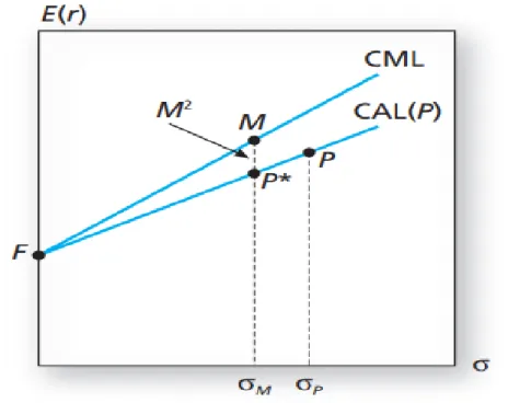
In 1997, Leah and Franco Modigliani developed the risk-adjusted performance measurement, perhaps better known as “RAP” or as the M2_{. The Modigliani} measurement assumes asset risk as the standard deviation, and takes influence from the Sharpe ratio, which was previously developed. However, the Sharpe ratio lacks any analytical significance besides only being a ratio (Sharpe, 1994). The Modigliani risk-adjusted return is easier interpreted compared to other ratios such as the Sharpe or Treynor2, since the M2_{returns a risk-adjusted percentage,} where the risk is equivalent to the risk of the market-portfolio. This is illustrated in the figure below, where the Capital Market Line (CML) of both assets

originates at the risk-free rate.

The main strength of the Modigliani measure is that it tells us how much better or worse the portfolio performs when adjusting for risk. In other words, the

Modigliani risk-adjusted performance standardizes the risks by un-levering or levering the standard deviation and equate it to the benchmark. Therefore, the vertical distance between the Capital Market Line and the Capital Allocation Line (CAL) of the various portfolios can be easily compared, to determine the actual portfolio return per unit of risk (Modigliani & Modigliani, 1997).

2_{For more information on the Treynor or Sharpe-ratios, see Treynor, J. (1965). How to rate management of} investment funds. Harvard Business Review, 43(1), pp 63-75.

(16)

16

Figure 3. Image displaying the Modigliani risk-adjusted performance. Source: Bodie, Kane & Marcus (2010). Any shareholder is able to recognize the difference between two M2 measures that for instance, yield values of 3 percent and 4.5 percent. Whilst for example, two different Sharpe values such as 0.35 and -0.2 are more complicated to evaluate, besides that the positive one is better than the other (Modigliani & Modigliani, 1997). The M2 measurement is calculated as follows.

𝑀2 _{= (}𝜎𝑀 𝜎𝑃

) (𝑅_𝑃 − 𝑅_𝑓) + (𝑅_𝑓) = (𝜎𝑀 𝜎𝑃

) 𝑒_𝑝+ 𝑅_𝑓 (5) Where, the 𝜎_𝑀 and 𝜎_𝑃 denotes the standard deviation of the market and the

portfolio. (𝑅_𝑃− 𝑅_𝑓) denotes the mean difference between the portfolio return and the risk-free interest rate, usually given by the US 10-Year treasury bill.

Additionally, this is simplified to the ratio of the standard deviation’s multiplied by the mean excess return, 𝑒_𝑝 which is the portfolio yield subtracted by the risk-free interest rate and the market returns. At last, the risk-risk-free interest rate is added to the equation.

(17)

17

3.2.2 The Jensen Alpha

The Jensen Alpha is another risk measurement that originates from the Capital Asset Pricing Model, (CAPM)3. The concept of the measurement is to compare a number of portfolios with different risks, where the risk is defined as the β-value. For instance, if assuming two portfolios, a common investor would like to know which asset (in some sense) is best, given separate risk for each portfolio. The model provides absolute value (α) which is interpreted as such. If the Alpha is greater than zero, α > 0 subsequently, the portfolio has generated excessive returns given the risk it carries. Similarly, if the Alpha is negative, α < 0, it implies that the returns, do not compensate for the portfolio risk. The Jensen Alpha is calculated as the following equation,

𝛼 = 𝑅_𝑝− (𝑅_𝑓+ 𝛽(𝑅_𝑚− 𝑅_𝑓)) (6) Where 𝛼 denotes the Jensen Alpha-value, 𝑅_𝑝 denotes the mean of the realized portfolio return. 𝛽 implies the beta-value of the portfolio, also described as the systematic risk which, is computed by using equation seven. Finally, 𝑅_𝑚− 𝑅𝑓implies the mean of the market risk premium. Additionally, the Jensen Alpha will only be used as a numerical estimate, meaning that the computed Alphas will not be statistically tested (Jensen, 1968).

1 𝑛∑ 𝛽𝑖

𝑛

𝑖 = 1

(7) The chosen risk measures will be used to analyze the portfolio performance against the benchmark. The reason is to be able to analyze the risk-adjusted returns and possibly conclude whether the relative strength portfolios achieve better or worse performance than the benchmark.

3.3 Data Collection

This study will use quantitative data from the Nasdaq Stockholm OMX Large- Cap stock exchange. Furthermore, the study will examine the monthly stock prices for all stocks in the Large-cap exchange during the period of 2010-2020. Furthermore, only closing prices for each security were analyzed, the closing price

3_{For more information on the CAPM, see Fama & French, (2004). The Capital Asset Pricing Model: Theory and} Evidence. Journal of Economic Perspectives. 18 (3), pp 25–46.

(18)

18

is the price paid in the last transaction of the opening hours. Additionally, some corporations prefer to list several types of stocks called common and preferred stock. Since prices of these may differ and in some cases yield different returns, this study will incorporate both of these types.

Furthermore, the data collection is primarily based in Microsoft Excel, where the financial data was downloaded. Excel was chosen due to being a relatively simple approach to process the data with help of functions and statistical packages. The study is dependent on the tools and services that Excel provides. It is considered that Excel is a reliable source and therefore that the data is unbiased and correct. However, when managing vast amounts of data and figures there is always a possibility of miscalculations, errors, and other inaccuracies.

The financial data such as prices and 𝛽-values were downloaded using the [STOCKHISTORY] function, and afterwards ranked based on the returns of the respective J-month formation periods.

3.3.1 Selection of measuring period

The period between 2010-2020 was chosen primarily because of keeping the data manageable while still obtaining sufficient data observations. The dataset begins during the year 2010, shortly afterwards the financial crisis of 2007-2009, while it ends during the COVID-19 crisis that severely affected global markets. Another reason that this specific measurement period was chosen was to test the

hypothesis in various market conditions.

During the start of the sample period 90 stocks were listed in the large-cap list of the Stockholm stock exchange. This number increased as more corporations listed their stock, at the end of the sample period a total of 114 stocks were listed. Thus, this amounts to a maximum of 114 ∗ 120 , monthly observations which all were processed to fit JK-months.

Hence, the study implements four different J-month formation period as well as four different K-month holding periods, each portfolio will be examined and observed 16 times a year (4 ∗ 4). This amounts to 32 observations for both the buy and sell portfolios during the study. Consequently, the buy-sell portfolios are based on adding each individual JK-month observation. Furthermore, the full list

(19)

19

of securities examined in the study are available in the appendix, along with the number of times each stock was traded.

3.3.2 Selection of financial markets

The market examined in this study is the Swedish stock market and OMXSPI index as the benchmark. OMXSPI, or also called Stockholm all-share is an index, that weights all stocks listed on the Stockholm Stock Exchange. This serves as a relevant benchmark since it includes all stocks listed, which gives a clearer picture than for example the OMXS30 that only consists of the 30 most liquid stocks in the Stockholm stock exchange.

The OMXSPI is a price-index, and since this study excludes dividend payment returns, it is a well-fitting benchmark rather than a gross-index. The differences between the two index types are that a price-index measures the price

development while a gross-index measures dividend payments and price development combined. Additionally, the development for the benchmark OMXSPI is illustrated in the appendix.

The sample of stocks originates from the Large-cap list of Stockholm Stock Exchange. The reason that all Large-Cap stocks from the years of 2010-2020 were examined was because the stocks listed tend to have a longer history in the stock market. Consequently, data observations would be easier to obtain. Another reason is that Large-Cap stocks have a higher market-capitalization and liquidity, Mid and Small-cap stocks tend to be more illiquid than Large-Cap stocks which may cause problems such as increased volatility and standard deviation when analyzing longer time-series data.

The interest rate selected was the six-month Swedish short-term treasury bill. The main reason is that the six-month treasury bill roughly matches the holding period of the portfolios constructed. This is the only treasury bill that will be examined, the reason is due to simplifying the estimates. The data for the interest rate was based on daily observations during the years of 2010-2020. Furthermore, the 200-day rolling average of the treasury rate during the sample period, was estimated, and applied to the calculation of the risk measurements. For instance, during any JK-month portfolio through year 2010, applied the 200-day rolling average treasury bill to the calculation of the Jensen Alpha and the Modigliani

(20)

risk-20

adjusted performance. The identical process followed for the remaining JK-month portfolios. Hence, in order to reduce the deviations of the interest rate, and

produce better risk estimates, the 200-day rolling average interest rate was

calculated. Additionally, the risk-free interest rate and the rolling average interest rate during the sample period is illustrated in the appendix.

3.3.3 Calculation of returns

Simultaneously, the returns for all securities will be calculated according to,

𝑅 =𝑃𝑡− 𝑃𝑡−1

𝑃_𝑡 (8)

Where 𝑅 denotes the return for the asset, 𝑃𝑡 denotes the adjusted closing price of the asset during time t, which implies the asset price at the end of the K-month holding period when the portfolio is liquidated. 𝑃_𝑡−1 denotes the adjusted closing price of the asset during time 𝑡₋₁, meaning the asset price after the J-month formation period where the security is acquired. Adjusted returns imply that the returns take stock splits and divestitures into account.

Further explained, all stocks were observed and ranked for each J-month formation period, where 𝑃_𝑡−1 varied between the closing price for J12, or any other J-month price. Similarly, the 𝑃𝑡 varied for the different J-month holding periods. For instance, when examining the J6K9 portfolio it implies that 𝑃_𝑡−1 is the price of the security when it is acquired after the six-month J-period, and 𝑃_𝑡 implies the price of the security when it is liquidated after the 9-month K-period. Since the study examines multi-period returns, it is appropriate to use the

geometric average for the benchmark and portfolio returns, rather than the arithmetic average (Hillier, 2020). The geometric average return is calculated as follows,

𝐺_𝐴𝑅 = (1 + 𝑅₁) ∗ (1 + 𝑅₂) … ∗ (1 + 𝑅_𝑛)1𝑛_{− 1} (9)

Where, 𝑅₁ denotes the portfolio return for period 1 or, 𝑅_𝑛 which imply the portfolio return for year 𝑛. The formula is then raised to the power of 1

𝑛 and subtracted by 1.

(21)

21

3.3.4 Quantitative process

Furthermore, when the returns of all securities were estimated, the data was segmented into deciles. The deciles were ranked descending order where the top decile, referred as P1 were the stocks that performed worst and the bottom decile, called P10 were the top performers, for each respective J-month period.

Further, when evaluating the different stocks at the year of 2010, nine of the corresponding best performing equities during the formation period will be

acquired with equal weights into the buy-portfolio. Similarly, for the sell-portfolio the nine worst performing equities will be short sold. Consequently, when

approaching the latter, and recent years the portfolios consisted of 14 stocks each. After respective K-month period, the return of the portfolios was calculated and the corresponding return for the benchmark during the same period was subtracted to get the net return. For instance, if the portfolio possesses a holding period of six months, then the average benchmark value for the same six months would be subtracted.

As an example, the raw return for the J3K3 buy portfolio during the first quarter of 2010 was -10.2 percent. Subsequently, the market returns for the first quarter of 2010 was subtracted from the raw return, which imply that the J3K3 buy portfolio generated -8.65 percent during the period. Likewise, the identical calculation was done for the remaining portfolios.

Thereafter, the return for the buy-sell portfolio were computed by adding the returns for the buy portfolio with the sell portfolio for the various years. For instance, if the buy portfolio during the initial year generated 2 percent returns, and the sell portfolio generated -1 percent net return, both accounting for

benchmark returns. Consequently, this implies the buy-sell portfolio generated a profit of 1 percent during the year. The identical calculation was done for the remainder of the years, where the cumulative average for all JK-month portfolios was presented. Consequently, each relative strength portfolio would generate positive figures, if they generated above-market returns, while returning negative figures if not.

The reason that the monthly returns is presented, is due to the portfolios having different holding periods, the J3K3 portfolio, has an aggregate holding period of

(22)

22

30 months during the decade since the portfolio is liquidated after the second quarter during a year. However, the other portfolios have extended K-month periods. Similarly, as Jagadeesh & Titman (1993), the results are for the whole decade is presented as the average value of all JK-month portfolios.

3.4 Limitations

3.4.1 Survivorship Bias

This study will examine time-series stock market data, where the data sample excludes delisted corporations. When analyzing historical prices in the stock market, survivorship bias will be a factor that may interfere with the results and cause skewness (Elton, Gruber & Blake 1996). A typical example of survivorship bias is when analyzing any type of security, for example a stock or fund and exclude companies that been delisted.

Corporations may be delisted for various reasons such as mergers and

acquisitions, fraud or insolvency. Furthermore, a mutual fund may close or merge with another mutual fund, the outcome is that those funds with good performance throughout the years will outlast those that perform poor. Elton, Gruber & Blake (1996) estimates that survivorship bias caused a skewness between 0,7% – 1,5% of mutual fund performance.

This may affect the study considerably, if for example investing in a corporation that becomes insolvent, then the shareholders lose all their capital. Consequently, since this study does not examine the possibility of insolvency the results may be affected positively and seem to be higher than it would have if including delisted corporations.

This study does not examine mergers and acquisitions. When a corporation is considering acquiring a certain competitor or others, it often needs to pay a premium to the shareholders. Therefore, when excluding delisted companies, it may also affect the results negatively. The reason that this study excludes delisted corporations is that the data would be challenging to obtain and analyze (Hillier, 2020).

(23)

23

3.4.1 Transaction Costs

This study ignores transaction costs and taxes. Transaction costs are applied every time an investor buys or sells securities and may differ depending on the size of transaction, wealth, marketplace or stockbrokers. Another thing that may vary depending on several factors is taxes. Therefore, the study also ignores taxes, which is in accordance with the majority of financial research since they are specific to every investor.

The absence of transaction costs is similarly a factor that may misrepresent the results. It would be appropriate to include transaction cost, in order to returns, which account for the transaction costs. .

3.4.2 Dividends and other Financial Securities

This study does also exclude dividend payments. Dividends are important to investors since it generates a balanced cash-flow during the investment period. Since corporations may decide to pay dividends to shareholders for different reasons, it may be difficult to track all. When dividends are paid to investors, the market-capitalization drops which also leads to a drop in the share price.

The effects of the dividend payments in this study, differ depending on when the certain corporation is bought or sold. If the stock is bought before a dividend payment, then the result is negative returns for the portfolio since the stock price decreases. If the stock is sold short before a dividend payment then the result is positive for the portfolio, while ignoring transaction costs associated with dividend payments in short positions (Hillier, 2020).

When short selling any given stock that pays dividends during the period that the stock is sold, the investor is required to pay the dividend amount to the lender. While the investor that owns shares of any corporation that pays dividends is able to obtain the amount (Hillier, 2020). Hence, assuming that both the buy and sell portfolios return approximately equal amounts of dividends, the effects of dividend payments for the buy-sell portfolio should be close to zero.

Corporations may also issue warrants or convertible bonds to investors. These assets lead to share dilution. Share dilution occurs when the corporation issues new shares which leads to a lower share price since the market-capitalization is

(24)

24

divided by an increased number of shares. The study ignores to examine share issuing, warrants and convertible bonds (Hillier, 2020).

3.4.3 Fundamental Causes

Consequently, this study does not examine fundamental reasons or factors that causes a certain stock to depreciate or appreciate. Corporations may issue new stocks, warrants, or decide to pay dividends, these reasons affect the stock price either positively or negatively. Therefore, analyzing securities prices without any context or insight to circumstances is not ideal.

4. Results

The results from the relative strength method implemented on Swedish stock market data are presented in the table below. Where the J denotes the formation period and K the holding period. The table is arranged so that the Buy represents the portfolio which bought the stock of J-month best performers and similarly, Sell represents the portfolio that sold the stock of the worst performers. The Buy-Sell implies the combined performance of both portfolios the respective portfolios while α and 𝑀2_{denotes the Jensen Alpha and the Modigliani risk-adjusted}

performance of the respective portfolio.

The average monthly return for each equal weighted portfolio is presented while also accounting for the benchmark yield as well. The t-statistics are displayed in parenthesis, while “*” implies significance for a five percent significance-level.

J K3 K6 K9 K12 3 Buy t-stat M2 α -1,73% (-2,640) -5,70% -2.52% -0,66% (-1,303) -1,41% -1,46% 0,46% (2,254) * 0,85% -0,34% 0,38% (2,477) * 0,57% -0,43% 3 Sell t-stat M2 α -0,55% (-4,355) -1,60% -1.34% -1,20% (-2,044) -2,03% -1,97% -1,56% (-4,917) -2,18% -2,34% -1,25% (-5,625) -2,01% -2,03% 3 Buy – sell t-stat 𝐌𝟐 α -2,28% (-5,531) -7,29% -3,07% -1,86% (-2,184) -3,57% -2.64% -1,10% (-2,038) -1,48% -1,89% -0,87% (-1,574) -0,77% -1,66% 6 Buy t-stat M2 α -1,92% (-4,143) -0,19% -2,72% 0,41% (3,310) * -0,26% -0,39% 0,48% (3,109) * 0,70% -0,32% 1,21% (3,933) * 0,83% 0,40%

(25)

25 6 Sell t-stat M2 α -1,87% (-3,930) -4,42% -2,66% -2,13% (-4,651) -3,91% -2,90% -1,48% (-4,389) -2,07% -2,26% -1,45% (-3,561) -1,46% -2,23% 6 Buy – Sell t-stat 𝐌𝟐 α -3,79% (-5,837) -0,83% -4,58% -1,72% (-2,818) -0,26% -2,50% -1,00% (-1,064) -1,02% -1,79% -0,24% (-0,908) 0,02% -1,03% 9 Buy t-stat M2 α 1,97% (3,933) * 2,59% 1,18% 1,23% (1,051) 1,78% 0,43% 1,10% (1,491) 1,37% 0,30% 0,44% (0,827) 0,58% 0,37% 9 Sell t-stat M2 α -0,48% (-6,009) -0,87% -1,27% -2,25% (-6,044) -4,44% -3.02% -1,55% (-4,081) -2,31% -2,33% -0,90% (2,518) -1,71% -1,68% 9 Buy – Sell t-stat 𝐌𝟐 α 1,49% (2,324) * 2,33% 0,70% -1,02% (-2,113) 1,36% -1,80% -0,45% (-0,811) -0,39% -1,24% -0,46% (-0,337) -0,34% -1,25% 12 Buy t-stat M2 α 1,14% (2,893) * 0,51% 0,35% 1,64% (3,422) * 0,48% 0,84% 1.24% (3,199) * 0,31% 0,44% 1,64% (3,427) * 0,25% 1,13% 12 Sell t-stat M2 α -0,67% (-1,776) 0,04% -1,46% -0,05% (-0,354) 0,29% -0,82% 1,01% (2,234) * 0,15% 0,23% -0,03% (-2,857) 0,14% -0,81% 12 Buy – Sell t-stat 𝐌𝟐 α 0,47% (0,745) 0,53% -0,32% 1,59% (2,592) * 0,38% 0,60% 2,25% (3,704) * 0,32% 1,46% 1,67% (2,418) * 0,26% 0,88%

Table 1. The relative strength portfolio based on the Jegadeesh Titman (1993), J-month formation period and the K-month holding period.

It appears that the respective portfolios give asymmetrical results. As a consequence, the combination of both, the buy-sell strategy provides rather interesting results. The maximum profit generated using the relative strength method was 2.25 percent while the maximum loss was 3,79 percent.

When examining the three different sets of portfolios, the majority of buy portfolios generated positive returns. In particular, 13 of 16 buy portfolios generated positive returns even though subtracting the market returns for the various years. Additionally, ten of these returns were statistically significant. Furthermore, the majority of sell portfolios managed to generate negative returns, even though adjusting for market returns, which cancel out the historically upward

(26)

26

trending market. In specific, 15 of 16 sell portfolios generated negative returns, with the exception of the J12K9 strategy, which managed to generate positive returns.

The buy-sell portfolios are able to provide consistent positive yields for the J12 strategy, for all K-month periods. Additionally, the J9K3 buy-sell portfolio yields rather high and positive returns. The remaining portfolios fail to provide any positive returns, but rather consistent negative yields. In total 5 of 16 buy-sell portfolios generated positive and significant returns. It appears that those buy portfolios that were sufficiently profitable were affected by the bigger drawdown from the various sell portfolios so that the majority of the buy-sell portfolios were negative.

Since the table only display the average monthly value for each JK-month portfolio, the annual returns for the J12K12 portfolio are presented in appendix where the buy, sell and buy-sell returns are displayed independently along with the benchmark returns.

Overall, the method is able to generate significantly profitable returns, for only a few strategies, and otherwise fail for the majority of strategies. The only strategy that managed consistent returns is the J12 strategy. Thus, the relative strength method is unable to consistently generate significant and positive results.

Furthermore, if an investor seeks to benefit from the relative strength method the effect of transaction costs needs to be considered. This is particularly important when selling stocks short since interest payments may be expensive.

4.1 Risk Evaluation

With the exception of the J12 and J9K3 strategy, the buy-sell portfolios produced negative returns given the risk they carried. The majority of portfolios created using the relative strength method have negative Jensen Alpha values. This indicates that the portfolio, given its systematic risk has underperformed

compared to the market returns. In other words, the returns of respective portfolio do not validate the risk the investor takes. The Jensen Alpha is on average -1.25% for the buysell portfolio, while the average is 0.24% for the buy portfolio and -1,81% for the sell portfolio. Therefore, during the years examined the

(27)

market-27

portfolio produces better returns, given the risk it holds compared to the relative strength portfolios.

The Modigliani risk-adjusted measurement also show negative returns when accounting for the standard deviation. The Modigliani risk-adjusted performance was on average -0,84% for the buy-sell portfolio, while -1,67% for the sell portfolio and 0,20% for the buy portfolio. It is notable that the M2_measurements are adding the risk-free interest rate net portfolio return. Therefore, it may seem that the portfolios performed better than expected. Furthermore, the J12 is slightly profitable even though to the massive return it generated during the final year. In Addition, the estimated β-values along with the standard deviation for each JK portfolio are found in the appendix 7.3 and 7.4.

Overall, seven buy-sell portfolios generated positive M2_{measurements. Similarly,} as the Jensen Alpha, the M2 of the numerous portfolios based on the relative strength method is unable, for the most part to generate sufficient returns in order to rationalize the risk involved.

4.2 Discussion

As previously acknowledged, the relative strength method implemented in this study would be perceived as successful if able to generate consistent above-market returns. Thus, since lacking consistency the strategy is considered unsuccessful.

The previous studies that used the relative strength method of investment, despite different time-horizons managed to achieve positive yields. In contrast to

Jagadeesh & Titman (1993), De Bondt & Thaler (1985), George & Hwang (2004) and Moskowitz & Grinblatt (1999) this study does not find any consistent profits. Additionally, these studies found profits for both the buy and the sell portfolios whilst this study found the opposite, namely to negative yields for all sell portfolios with exception of one. The results are similar to the findings of

Rouwenhorst (1997), who could not obtain significant profits in the Swedish stock market.

The conclusions of the Jagadeesh & Titman (1993) were that the returns generated was not explained by the β-values of the respective portfolios. However, this

(28)

28

study finds the opposite. The majority of portfolios yield negative returns when accounting for the β-values. This study also finds that the estimated returns of the portfolios do not generate sufficient results in order to justify for the standard deviation. Consequently, the relative strength method is unable to consistently generate excess returns during the sample period. Any investor could rather simply increase the risks of their holdings and expect higher yield, but the challenge remains to account for the risk so that the expected return is sufficient. The relative strength method was unable to achieve this.

5. Conclusion

The aim of the study was to examine the relative strength investment method and investigate whether it contradicts the Efficient Market Hypothesis. In order to do this, the relative strength method essentially needed to be sufficiently and

consistently profitable. The study implemented the identical relative strength strategies as Jagadeesh & Titman (1993) however, this study applied the various strategies on Swedish stock market data during the decade of 2010-2020. The results were also evaluated from a perspective, by using two distinct risk-measurements.

The findings were similar as Rouwenhorst (1997) underwhelming. The relative strength method managed to generate excess return for a few strategies but failed to do this consistently. When evaluating the raw data, a substantial number of stocks in the sell portfolio reversed their trend rather fast. This may be the reason that nearly all of the sell portfolios yielded negative returns, this is also in

accordance with the findings of De Bondt & Thaler (1985).

The relative strength method, despite several variations certainly enhances the debate of whether the Efficient Market Hypothesis is valid or not. The reason for this is that it occasionally manages to generate excess returns similar to the previous research however, this was not the case for this specific study. Perhaps, the various studies that showed substantial profits transpired to choose the appropriate sample period that suits their thesis, as Malkiel (2003) claims. In addition, perhaps this study failed to show consistent profits, because of a weak-form efficient stock market in Sweden as Worthington & Higgs (2004)

(29)

29

Thus, this study fails to reject the null hypothesis, which is expressed in the first equation. One can observe that the study managed to reject the null hypothesis in a few cases, as the buy-sell portfolio was able to generate excess returns.

However, this will not be done since the method was unable to provide consistency.

Finally, for the matter of further research, it would be interesting to perform a similar study which applies the relative strength method for common and

preferred stocks. When constructing the study, it was often common that the class A and respectively, the class B stock of the same corporation was trading at distinct disproportion. This is also known as a spread between the stocks. If for instance, selling the highest trading stock and buying the lowest trading stock, perhaps both stocks would unite at a smaller deviation. Hence the spread between the two securities perhaps would decrease.

(30)

30

6. References

Bodie, Z. Kane, A. Marcus, A. (2010). Investments. McGraw Hill Higher Education.

Brealey, R. (2019). Principles of Corporate Finance. McGraw-Hill Higher Education.

De Bondt, F.M. & Thaler, R. (1985). Does the Stock Market Overreact? The Journal of finance, 40(3), pp 793-805.

Dreman, D. & Berry, M. (1995). Overreaction, underreaction, and the low p/e effect. Financial Analysts Journal, 51(4), pp 21-30

Elton, E. Gruber, M. & Blake, C. (1996). Survivor Bias and Mutual Fund Performance. The Review of Financial Studies, 9(4), pp 1097–1120.

Fama, E. (1970). Efficient capital markets: a review of theory and empirical work. Journal of finance, 25(2), pp 383-417.

French, K. Roll, R. Stock Return Variances: The Arrival of Information and the Reaction of Traders. Journal of Financial Economics. 17(1). pp 1-5.

George, TJ. Hwang, C-Y. (2004) The 52-Week High and Momentum Investing. The Journal of finance, 59(5), pp 2145-2176.

Grossman, S. Stiglitz, J. (1980). On the Impossibility of Informationally Efficient Market. The American Economic Review, 70 (3), pp. 393-408

Hillier, D. Ross, S. Westerfield, R. Joffe, J. Jordan, B. (2020). Corporate Finance, Fourth European Edition. McGraw-Hill Education Ltd.

Jagadeesh, N. Titman, S. (1993). Returns to Buying Winners and Selling Losers: Implications for Stock Market Efficiency. Journal of finance, 48(1), pp 65-91. Jensen, M. (1968). The Performance of Mutual Funds in the Period 1945-1964. The Journal of Finance, 23(2), pp 389-416.

Jung, J. Shiller, R. (2006). Samuelsson’s Dictum And The Stock Market. Cowles Foundation For Research in Economics, Yale University, 43(2), pp 219-228. Keown, A. Pinkerton, J. (1981). Merger Announcements and Insider Trading Activity. Journal of Finance, 36(4), pp 855-869.

(31)

31

Keynes, J-M. (1936). The General Theory of Employment, Interest and Money. Malkiel, B. (2019). A Random Walk Down Wall Street; The time-tested strategy for successful investing. WW Norton Co.

Malkiel, B. (2003). The Efficient Market Hypothesis and Its Critics. The Journal of Economic Perspectives, 17(1). pp 59-82.

Modigliani, F. Modigliani, L. (1997). Risk-Adjusted Performance. The Journal of Portfolio Management. 23(2), pp 45-54.

Moskowitz, T. Grinblatt, M. (1999). Do Industries Explain Momentum. The Journal of Finance, 54(4), pp 1249-1290.

OECD (2021), Short-term interest rates (indicator).

https://data.oecd.org/interest/short-term-interest-rates.htm (Accessed on 19 May 2021).

Parmler, J. Gonzalez, A. (2007). Is Momentum Due to Data-snooping. The European Journal of Finance, 13(7). pp 301-318.

Rouwenhorst, K.G. (1997). International Momentum Strategies. The Journal of Finance, 53(1), pp 267-284.

Sharpe. W. (1994). The Sharpe Ratio. The Journal of Portfolio Management, 21(1), pp 49-58.

Shiller, R. (2016) Irrational Exuberance, Revised and expanded third edition.

Princeton University Press.

Studenmund, A-H. (2017). A Practical Guide to Using Econometrics, Global Edition. Pearson Education Limited.

Worthington, A. Higgs, H. (2004). Random walks and market efficiency in European equity markets. Global Journal of Finance and Economics 1(1), pp. 59-78.

(32)

32

7. Appendix

7.1 All securities examined in the study

Corporation Ticker Nr of

trades Corporation Ticker

Nr of trades

AAK AB AAK 9 EQT AB EQT 1

Abb Ltd ABB 8 Telefonaktiebolaget LM Ericsson ERIC B 11

Addtech AB ADDT B 8 Essity AB ESSITY A 0

Ahlström-Munksjö Oyj AM1S 2 Evolution Gaming Group AB EVO 13

Alfa Laval AB ALFA 2 Fabege AB FABG 4

Arion banki hf ARION SDB 1 FastPartner AB FPAR D 0 Arjo AB ARJO B 4 Fenix Outdoor International Ltd. FOI B 8

Assa Abloy AB ASSA B 8 Getinge AB GETI B 12

ASTRAZENECA PLC AZN 7 Svenska Handelsbanken AB SHB B 6 Atlas Copco AB ATCO A 6 H & M Hennes & Mauritz AB HM B 8

Atlas Copco AB ATCO B 7 Hexagon AB HEXA B 4

Atrium Ljungberg AB ATRLJ B 0 Hexpol AB HPOL B 12

AUTOLIV, INC. ALIV SDB 8 Holmen AB HOLM A 4

Avanza Bank Holding AB AZA 8 Holmen AB HOLM B 5

Axfood AB AXFO 6 Hufvudstaden AB HUFV A 2

Beijer Ref AB BEIJ B 10 Husqvarna AB HUSQ A 10

Betsson AB BETS B 11 Husqvarna AB HUSQ B 10

BHG Group AB BHG 3 ICA Gruppen AB ICA 7

BillerudKorsnas AB BILL 5 Industrivarden AB INDU C 3

Boliden AB BOL 14 Indutrade AB INDT 1

Bravida Holding AB BRAV 2 Intrum AB INTRUM 6

Bure Equity AB BURE 5 Investor AB INVE B 0

Castellum AB CAST 2 JM AB JM 5

Catena AB CATE 7 KINDRED GROUP PLC KIND

SDB 14

Cint Group AB CINT 0 Kinnevik AB KINV A 4

Dometic Group AB DOM 4 Klövern AB KLOV A 2

Electrolux AB ELUX A 15 Kungsleden AB KLED 6

Elekta AB EKTA B 12 Investment AB Latour LATO B 4

Epiroc AB EPI A 0 Lifco AB LIFCO B 8

L E Lundbergforetagen AB LUND B 7 Loomis AB LOOMIS 6

Lundin Energy AB LUNE 16 Securitas AB SECU B 2

Lundin Mining Corporation LUMI 13 Sinch AB SINCH 12

Medicover AB MCOV B 2 Skanska AB SKA B 5

Millicom International Cellular SA TIGO SDB 8 SKF Inc SKF A 12

Mycronic AB MYCR 18 SKF Inc SKF B 10

NCC AB NCC A 5 SSAB AB SSAB A 15

NCC AB NCC B 5 SSAB AB SSAB B 15

Nibe Industrier AB NIBE B 8 Stora Enso Oyj STE R 8

Nobia AB NOBI 14 Sweco AB SWEC B 6

Nokia Corporation NOKIA SEK 15 Swedbank AB SWED A 6

(33)

33

Nordea Bank Abp NDA SE 6 Swedish Orphan Biovitrum AB SOBI 12

Nordnet AB SAVE 0 Tele2 AB TEL2 A 5

Nyfosa AB NYF 2 Telia Company AB TELIA 4

Pandox AB PNDX B 0 Thule Group AB THULE 10

Peab AB PEAB B 2 TietoEVRY Corporation TIETOS 0

PFIZER INC. PFE 8 Traton SE 8TRA 0

Platzer Fastigheter Holding AB PLAZ B 4 Trelleborg AB TREL B 8

Ratos AB RATO A 9 Wallenstam AB WALL B 3

Resurs Holding AB RESURS 0 VEONEER, INC. VNE SDB 5

Saab AB SAAB B 6 Wihlborgs Fastigheter AB WIHL 2

Sagax AB SAGA PREF 1 Vitrolife AB VITR 8

Samhallsbyggnadsbolaget I Norden

AB SBB D 0 Volvo AB VOLV B 6

Sandvik AB SAND 6 ÅF Pöyry AB AF B 2

Svenska Cellulosa SCA AB SCA A 8

Svenska Cellulosa SCA AB SCA B 8

Skandinaviska Enskilda Banken AB SEB A 2

Skandinaviska Enskilda Banken AB SEB C 3

SECTRA AB SECT B 10

7.2 Graph of the annual return of the J12K12 portfolio

-60,00% -40,00% -20,00% 0,00% 20,00% 40,00% 60,00% 80,00% 100,00% 120,00% 140,00% 160,00% 2011 2012 2013 2014 2015 2016 2017 2018 2019 2020

(34)

34

7.3 Graph of the respective β-values for the portfolios

7.4 Chart visualizing the standard deviation (σ) of the portfolios 0,950 1,000 1,050 1,100 1,150 1,200 1,250

Buy Sell Zero-cost

0,0% 20,0% 40,0% 60,0% 80,0% 100,0% 120,0% 140,0% 160,0% 180,0%

(35)

35

7.5 Figure of benchmark, OMXSPI

7.6 Figure of the risk-free interest rate

Source: OECD (2021). 0 100 200 300 400 500 600 700 800 900 -1,50% -1,00% -0,50% 0,00% 0,50% 1,00% 1,50% 2,00% 2,50%

The (in)efficiency of Financial Markets : Applying the Relative Strength Strategy on the Swedish Large cap Exchange