On the Use of Accuracy and Diversity Measures for
Evaluating and Selecting Ensembles of Classifiers
Tuve LöfströmSchool of Business and Informatics University of Borås tuve.lofstrom@hb.se
Ulf Johansson
School of Business and Informatics University of Borås ulf.johansson@hb.se
Henrik Boström Informatics Research Centre
University of Skövde henrik.bostrom@his.se
Abstract
The test set accuracy for ensembles of classifiers selected based on single measures of accuracy and diversity as well as combinations of such measures is investigated. It is found that by combining measures, a higher test set accuracy may be obtained than by using any single accuracy or diversity measure. It is further investigated whether a multi-criteria search for an ensemble that maximizes both accuracy and diversity leads to more accurate ensembles than by optimizing a single criterion. The results indicate that it might be more beneficial to search for ensembles that are both accurate and diverse. Furthermore, the results show that diversity measures could compete with accuracy measures as selection criterion.
1. Introduction
An ensemble is a composite model aggregating multiple base models, making the ensemble prediction a function of all included base models. Ensemble learning, consequently, refers to methods where a target function is learnt by training and combining a number of individual models.
Although the use of Artificial Neural Networks (ANNs) will most often lead to very accurate models, it is also well known that even higher accuracy can be obtained by combining several individual models into ensembles; see e.g.,[1,2]. The main reason for the increased accuracy obtained by ensembles is the fact that uncorrelated base classifier errors will be eliminated when combining several models using averaging; see e.g. [3]. Naturally, this requires the base classifiers to commit their errors on different instances – there is nothing to gain by combining identical models. Informally, the key term diversity therefore means that the base classifiers make their mistakes on different instances.
While the use of ensembles is claimed to virtually guarantee increased accuracy compared to the use of single models, the problem of how to maximize ensemble accuracy is far from solved.
The purpose of this study is to look into ensemble member selection based on performance on training data. More specifically, the assumption is that we have a number of individually trained ANNs, and the task is to select a subset of these to form an ensemble. Naturally, what we would like to maximize is ensemble accuracy, when applying the ensemble to novel (test) data. The performance measures considered in this study, either in isolation or in combination, to select an ensemble are base classifier accuracy, ensemble accuracy and the two diversity measures double fault and difficulty.
In the next section, the background of this study is presented together with related work. In section 3, the method of the study is described, which is followed by an analysis of the results in section 4. Finally, concluding remarks are given in section 5.
2. Background and related work
Krogh and Vedelsby derived an equation stating that the generalization ability of an ensemble is determined by the average generalization ability and the average diversity (ambiguity) of the individual models in the ensemble [4]. More specifically; the ensemble error, E, can be calculated using
E =E − (1) A
whereE is the average error of the base models and A is the ensemble diversity, measured as the weighted average of the squared differences in the predictions of the base models and the ensemble. Since diversity is always positive, this decomposition proves that the ensemble will always have a higher accuracy than the average accuracy obtained by the individual classifiers. The problem is, however, the fact that the two terms are normally highly correlated, making it necessary to balance them rather than just maximizing diversity.
For classification, where a zero-one loss function is used, it is, however, not possible to decompose the ensemble error into error rates of the individual classifiers and a diversity term. Instead, algorithms for ensemble creation typically use heuristic expressions trying to approximate the unknown diversity term.
Naturally, the goal is to find a diversity measure highly correlated with majority vote accuracy.
Kuncheva presents a review of previous work where diversity in some way has been utilized to select the final ensemble [5]. Giacinto and Roli [6] form a pair-wise diversity matrix using the double fault measure and the Q statistic [7] to select classifiers that are least related. They search through the set of pairs of classifiers until the desired number of ensemble members is reached. Likewise, Margineantu and Dietterich [8] also search for the pairs of classifiers with lowest kappa (highest diversity) from a set of classifiers produced by AdaBoost. They call this approach “ensemble pruning”.
Giacinto and Roli [9] apply a hierarchical clustering approach were the ensembles are clustered based on pair-wise diversity. The ensemble is formed by picking a classifier from each cluster and step-wise joining the two least diverse classifiers until all classifiers belong to the same cluster. The ensemble used in the end is the ensemble with highest accuracy on a validation set.
Banfield et al. [10] use an approach were only the uncertain data points are considered and used to exclude classifiers failing on a larger proportion of these instances, compared to other classifiers.
All these approaches select ensembles based on diversity between pairs of classifiers, rather than on ensemble diversity.
Several studies have shown that all diversity measures evaluated show low or very low correlation with ensemble test set accuracy; see e.g. [11,12]. As a consequence, diversity measures are expected to be poor predictors for test set accuracy. The measures double fault and difficulty does, however, constantly perform better than the other measures.
3. Method
The purpose of this study is to evaluate combinations of measures that could be used to estimate ensemble accuracy on novel (test) data. More specifically, we investigate the following four measures, either separately or somehow combined: ensemble accuracy (EA), base classifier accuracy (BA), and the diversity measures double-fault (DF) and difficulty (DI). Accuracy refers to the accuracy of the entire ensemble on a dataset. Base classifier accuracy refers to the average accuracy obtained by the base classifiers on a dataset.
Let the output of each classifier Di be represented by an N-dimensional binary vector yi, where the jth element yj,i=1 if Di recognizes correctly instance zj and 0 otherwise, and let Nab refer to the number of instances for which yj,i=a and yj,k=b, e.g., N11 is the number of instances correctly classified by both
classifiers. Using this notation, the double fault diversity measure, which is the proportion of instances misclassified by both classifiers, is defined as
00 , 11 10 01 00 i k N DF N N N N = + + + (2)
For an ensemble consisting of L classifiers, the averaged double fault (DF) over all pairs of classifiers is 1 , 1 1 2 ( 1) L L av i k i k i DF DF L L − = = + = −
∑ ∑
(3)The difficulty measure was used in [13] by Hansen and Salomon. Let X be a random variable taking values in {0/L, 1/L,…, L/L}. X is defined as the proportion of classifiers that correctly classify an instance x drawn randomly from the data set. To estimate X, all L classifiers are run on the data set. The difficulty θ is then defined as the variance of X. The reason for including only these two diversity measures is simply the fact that they have performed slightly better than other measures in previous studies; see [11].
3.1. Ensemble Settings
Three sets of ANNs, with 15 networks in each, were trained initially. The first set of ANNs did not have any hidden layer at all, thus resulting in rather weak models. The ANNs in the second set had one hidden layer and the number of units in the hidden layer was based on data set characteristics according to (4).
2 ( )
h=
⎢
⎢
⎣
rand⋅ v c⋅⎥
⎥
⎦
(4)where v is the number of input variables, c is the number of classes, and rand is a random number in the interval [0, 1]. This set represents a standard setup for ANN training.
The third set of ANNs used two hidden layers, where h1 in (5) determines the number of units in the
first hidden layer and h2 in (6) determines the number
of units in the second layer.
1 ( ) / 2 4 ( ( ) / )
h =
⎢
⎣
⎢
v c⋅ + rand⋅ v c⋅ c⎥
⎥
⎦
(5)2 ( ( ) / )
h =
⎢
⎢
⎣
rand⋅ v c⋅ c +c⎥
⎥
⎦
(6)As before, v is the number of input variables and c is the number of classes. The third set of models could be expected to be over-fitted on the training set. The motivation of using two-layered networks in an ensemble is that over-fitted models may not be detrimental for the overall performance. In fact, extensive experimentation shows that for ensembles, over-fitted models are preferable over more well-fitted models.
All data except the test data was used to train the ANNs. For actual experimentation, 10-fold
cross-validation was used. All ANNs were trained without early stopping validation, which may also lead to slightly over-fitted models. Each network used only 80% of the available variables, drawn randomly. Majority voting was used to determine ensemble classifications.
Overall, it should be noted that the design choices were made to ensure some diversity among the networks in each group.
3.2. Experiments
The empirical study was divided into three experiments. The purpose of the first experiment was to evaluate both single measures and linear combinations of measures. Although the concept of combining diversity measures may appear somewhat odd, it must be noted that the diversity measures capture very different properties. Furthermore, combining accuracy measures with diversity measures fits very well into the original Krogh-Vedelsby idea, i.e., that ensembles should consist of accurate models that disagree in their predictions. On the other hand, it is not obvious exactly how to formulate such a combination, especially since the measures have different ranges and meanings. In this experiment, we chose the simple approach of just summing the measures that are to be combined. For some diversity measures where a lower value indicates a higher degree of diversity, this, of course, means subtracting instead of adding the value. As an example, a combination of ensemble accuracy (↑), base classifier accuracy (↑) and double fault (↓) would be:
S EA BA DF= + − (7)
In the first experiment, 10,000 random ensembles with exactly 25 ANNs were drawn. The test set accuracy of the best performing ensemble, according to the individual or combined measures, is reported.
In the second and third experiments, GA was used to search for ensembles that simultaneously optimize both an accuracy measure and a diversity measure, using Matlabs multi-objective GA function, gamultobj1. The second experiment did not impose any restrictions on the size of an ensemble, other than that it should consist of at least two ANNs. In the third experiment, the sizes of the ensembles were restricted to consist of at least 25 ANNs. The second and third experiments used the same ANNs as in the first experiment.
The default settings for Matlab’s GA toolbox were used when running the GA, except for the settings described in Table 1.
1
As part of the Genetic Algorithm and Direct Search Toolbox™ 2.3: http://preview.tinyurl.com/gamultobj
Table 1. GA settings
Parameter Value
Population Type Bit string
Population Size 200
Generations 100
Pareto Fraction 0.5
Each gene in the GA is a bit string of length 45, where a 1 in any location indicates that the ANN with corresponding index should be included in the ensemble.
Let A={ , , }a1… am be a set of alternatives
(ensembles in our case) characterized by a set of criteria C={ , ,C1… CM} (accuracy and diversity in our case). The Pareto-optimal set S∗ S
⊆ contains all non-dominated alternatives. An alternative ai is non-dominated iff there is no other alternativeaj∈S j, ≠i,
so that aj is better than ai on all criteria. The Pareto fraction option limits the number of individuals on the Pareto front.
From among the solutions generated by GA that reside in the Pareto front, three ensembles are selected. The two ensembles with best performance with respect to the accuracy measure and to the diversity measure are selected. These two ensembles correspond to the two edges of the Pareto front and are almost the same as would be found if optimizing only one of the objectives. The only difference to single objective search is that if there are ties, the ensemble with best performance on the second objective is guaranteed to be selected, which would not be the case in single objective search. The third model selected is the one closest to the median of the ensembles in the Pareto front along both measures. The Euclidian distance is used to find the ensemble closest to the median. This ensemble is selected, since it represents both one of the most accurate ensembles and at the same time one of the most diverse.
3.3. Data Sets
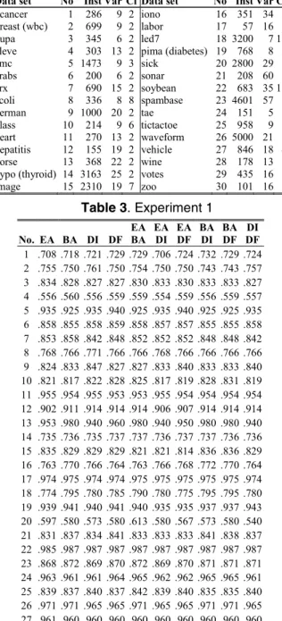
This study used 27 data sets from the UCI Repository [14]. For a summary of the characteristics of the data sets, see Table 2. The first column, No is a numbering used in the result tables instead of abbreviations. Inst is the total number of instances in the data set. Cl is the number of output classes in the data set. Var is the number of input variables.
Table 2. Characteristics of data sets used
Data set No Inst Var Cl Data set No Inst Var Cl
bcancer 1 286 9 2 iono 16 351 34 2
breast (wbc) 2 699 9 2 labor 17 57 16 2
bupa 3 345 6 2 led7 18 3200 7 10
cleve 4 303 13 2 pima (diabetes) 19 768 8 2
cmc 5 1473 9 3 sick 20 2800 29 2 crabs 6 200 6 2 sonar 21 208 60 2 crx 7 690 15 2 soybean 22 683 35 19 ecoli 8 336 8 8 spambase 23 4601 57 2 german 9 1000 20 2 tae 24 151 5 3 glass 10 214 9 6 tictactoe 25 958 9 2 heart 11 270 13 2 waveform 26 5000 21 3 hepatitis 12 155 19 2 vehicle 27 846 18 4 horse 13 368 22 2 wine 28 178 13 3
hypo (thyroid) 14 3163 25 2 votes 29 435 16 2
image 15 2310 19 7 zoo 30 101 16 7 Table 3. Experiment 1 No. EA BA DI DF EA BA EA DI EA DF BA DI BA DF DI DF 1 .708 .718 .721 .729 .729 .706 .724 .732 .729 .724 2 .755 .750 .761 .750 .754 .750 .750 .743 .743 .757 3 .834 .828 .827 .827 .830 .833 .830 .833 .833 .827 4 .556 .560 .556 .559 .559 .554 .559 .556 .559 .557 5 .935 .925 .935 .940 .925 .935 .940 .925 .925 .935 6 .858 .855 .858 .859 .858 .857 .857 .855 .855 .858 7 .853 .858 .842 .848 .852 .852 .852 .848 .848 .842 8 .768 .766 .771 .766 .766 .768 .766 .766 .766 .766 9 .824 .833 .847 .827 .827 .833 .840 .833 .833 .840 10 .821 .817 .822 .828 .825 .817 .819 .828 .831 .819 11 .955 .954 .955 .953 .953 .955 .954 .954 .954 .954 12 .902 .911 .914 .914 .914 .906 .907 .914 .914 .914 13 .953 .980 .940 .960 .980 .940 .950 .980 .980 .940 14 .735 .736 .735 .737 .737 .736 .737 .737 .736 .736 15 .835 .829 .829 .829 .821 .821 .814 .836 .836 .829 16 .763 .770 .766 .764 .763 .766 .768 .772 .770 .764 17 .974 .975 .974 .974 .975 .975 .975 .975 .975 .974 18 .774 .795 .780 .785 .790 .780 .775 .795 .795 .780 19 .939 .941 .940 .941 .940 .935 .935 .937 .937 .943 20 .597 .580 .573 .580 .613 .580 .567 .573 .580 .540 21 .831 .837 .834 .841 .833 .833 .833 .841 .838 .837 22 .985 .987 .987 .987 .987 .987 .987 .987 .987 .987 23 .868 .872 .869 .870 .872 .869 .870 .871 .871 .871 24 .963 .961 .961 .964 .965 .962 .962 .965 .965 .961 25 .839 .837 .840 .837 .842 .839 .840 .835 .835 .840 26 .971 .971 .965 .965 .971 .965 .965 .971 .971 .965 27 .961 .960 .960 .960 .960 .960 .960 .960 .960 .960 R 7.4 6.5 7.6 6.6 5.8 8.6 7.8 5.8 5.8 7.5
4. Results
The results from the first experiment are presented in Table 3 and Table 4. The measures in the column header indicate which measures that are linearly combined and used to select the ensemble. As noted above, the No. column indicates the data set and corresponds to the numbering in Table 2. The last row show the mean ranks and is indicated with R. Lower ranks are better.
Table 4. Experiment 1, continued
No. EA BA DI EA BA DF EA DI DF BA DI DF EA BA DI DF 1 .732 .726 .721 .732 .729 2 .754 .754 .736 .746 .754 3 .830 .830 .827 .833 .830 4 .559 .556 .556 .556 .558 5 .925 .925 .935 .925 .925 6 .855 .855 .857 .854 .855 7 .848 .848 .848 .845 .848 8 .766 .766 .766 .766 .766 9 .820 .823 .840 .833 .827 10 .825 .825 .819 .828 .825 11 .953 .953 .954 .954 .953 12 .917 .917 .906 .911 .917 13 .980 .980 .940 .960 .960 14 .737 .736 .736 .733 .737 15 .829 .829 .821 .829 .829 16 .768 .762 .763 .771 .768 17 .975 .975 .975 .975 .975 18 .790 .790 .780 .800 .795 19 .940 .940 .935 .940 .938 20 .567 .620 .573 .560 .580 21 .835 .833 .833 .840 .837 22 .987 .987 .987 .987 .987 23 .871 .871 .870 .872 .871 24 .962 .962 .962 .965 .964 25 .842 .842 .840 .837 .842 26 .971 .971 .965 .971 .971 27 .960 .960 .960 .960 .960 R 6.6 7.2 9.2 6.5 5.9
The results achieved regarding the use of individual measures are interesting. Since the results reported here are from ensembles selected using the training data, we could expect a higher bias for the ensemble accuracy measure, which could explain why the average rank for ensemble accuracy is higher than for base classifier accuracy, even though the difference is not significant.
So far, most research has concluded that diversity measures are bad predictors for test set accuracy. Even though most studies agree that double fault and difficulty are the best among the diversity measures at predicting test set accuracy, it has been concluded that ensemble accuracy or base classifier accuracy are still superior. The results presented here indicate that these two diversity measures, if combined with the accuracy measures, very well could compete with the use of accuracy measures alone as selection criteria’s for ensembles.
The ensembles selected using combinations of at least two measures is often better than using a single measure. However, using only diversity measures, or using both diversity measures in combination with one
of the accuracy measures does not turn out to be very successful.
Another interesting result is that the combination of only accuracy measures (EA BA) is among the best solutions. This suggests that combining more than one performance measure could be beneficial.
No significant differences could, however, be observed.
Table 5. Experiment 2, ensemble size >= 2
EA DI EA DF BA DI BA DF
No. Med Acc Div Med Acc Div Med Acc Div Med Acc Div
1 .697 .703 .703 .703 .685 .691 .697 .671 .694 .703 .674 .697 2 .725 .719 .721 .725 .715 .706 .700 .632 .732 .729 .729 .718 3 .821 .836 .833 .820 .820 .820 .827 .807 .829 .825 .813 .827 4 .551 .550 .558 .548 .549 .543 .552 .541 .552 .557 .547 .549 5 .945 .945 .945 .945 .942 .942 .942 .942 .949 .940 .945 .945 6 .859 .859 .858 .862 .853 .851 .852 .857 .860 .852 .845 .864 7 .836 .842 .836 .836 .833 .837 .836 .830 .841 .842 .821 .836 8 .760 .761 .763 .757 .745 .741 .748 .736 .758 .755 .744 .761 9 .855 .853 .833 .840 .823 .811 .833 .793 .833 .850 .793 .833 10 .815 .820 .828 .817 .792 .804 .797 .781 .801 .798 .786 .817 11 .961 .963 .960 .960 .961 .959 .962 .952 .958 .958 .957 .957 12 .911 .911 .909 .911 .887 .884 .889 .892 .910 .909 .897 .911 13 .980 .980 .980 .980 .969 .969 .969 .969 .940 .940 .940 .940 14 .727 .732 .734 .702 .732 .729 .733 .724 .732 .737 .733 .706 15 .850 .850 .850 .850 .812 .805 .812 .812 .830 .814 .807 .850 16 .759 .757 .763 .763 .748 .742 .750 .729 .758 .753 .750 .762 17 .975 .974 .975 .976 .972 .974 .972 .970 .974 .974 .973 .976 18 .780 .780 .780 .780 .742 .743 .757 .717 .778 .780 .745 .775 19 .941 .941 .941 .941 .921 .928 .923 .896 .939 .943 .921 .943 20 .539 .538 .547 .540 .559 .557 .567 .573 .541 .550 .513 .553 21 .918 .918 .927 .919 .929 .932 .927 .916 .920 .922 .913 .919 22 .985 .985 .985 .985 .984 .984 .984 .983 .985 .986 .982 .985 23 .855 .856 .862 .849 .857 .858 .860 .831 .862 .863 .859 .849 24 .962 .962 .961 .962 .962 .964 .961 .966 .962 .964 .958 .962 25 .844 .843 .840 .845 .836 .831 .844 .794 .838 .844 .806 .845 26 .959 .959 .959 .959 .974 .974 .974 .974 .953 .953 .944 .957 27 .950 .950 .950 .950 .956 .956 .956 .956 .952 .956 .940 .950 R 3.1 2.9 3.5 5.5 4.7 7.5 3.6 7.3 3.9 7.5 8.1 8.3
The results from the second and third experiments are presented in Table 5 and Table 6. The first row in the column header indicates which two measures that were used as objectives in the GA search. The three columns for each pair of measures represent the median ensemble (Med) on the Pareto front, the most accurate ensemble based on the specific accuracy measure used (Acc), and the most diverse, based on the specific diversity measure used (Div). Table 5 shows the results from the second experiment.
The performance is obviously greatly affected by the choice of pairs of measures. Any combination that includes Base classifier accuracy or double fault is obviously not a very good choice, using these settings. Combinations including ensemble accuracy or difficulty turn out to be constantly good choices. The
most median ensemble turns out to be a good choice whenever any of the measures produces good results.
A Friedman test indicates significant difference with p = 0.05. A Nemenyi post-hoc test, with p = 0.05, has a critical difference of 3.2. This means that the five best ranked results are all significantly better than the five worst ranked. Moreover, the two worst ranked results are also significantly worse than selecting the most accurate ensemble using the combination of ensemble accuracy and double fault.
Table 6. Experiment 3, ensemble size >= 25
EA DI EA DF BA DI BA DF
No. Med Acc Div Med Acc Div Med Acc Div Med Acc Div
1 .717 .700 .709 .725 .712 .732 .726 .724 .724 .724 .726 .735 2 .741 .739 .736 .743 .739 .736 .729 .732 .736 .732 .732 .736 3 .824 .823 .827 .827 .823 .827 .836 .827 .823 .830 .823 .823 4 .551 .556 .552 .555 .554 .563 .559 .565 .554 .563 .565 .563 5 .945 .945 .945 .942 .942 .942 .935 .920 .945 .935 .930 .943 6 .859 .858 .862 .859 .858 .861 .858 .861 .861 .858 .862 .858 7 .845 .842 .842 .845 .845 .842 .842 .839 .839 .845 .842 .842 8 .775 .771 .769 .775 .770 .769 .772 .775 .769 .771 .775 .769 9 .835 .833 .840 .853 .847 .853 .847 .833 .847 .860 .833 .860 10 .804 .811 .803 .819 .819 .819 .817 .811 .806 .817 .822 .817 11 .959 .958 .958 .959 .959 .958 .957 .957 .958 .958 .957 .959 12 .920 .920 .920 .917 .917 .917 .917 .914 .920 .917 .909 .914 13 .980 .980 .980 .977 .977 .977 .960 .980 .960 .980 .980 .980 14 .734 .735 .737 .735 .736 .736 .737 .735 .735 .735 .735 .734 15 .829 .829 .829 .829 .828 .829 .843 .829 .850 .829 .821 .836 16 .768 .770 .768 .771 .768 .768 .764 .771 .767 .764 .774 .768 17 .976 .976 .976 .975 .975 .976 .975 .976 .976 .975 .975 .976 18 .775 .775 .775 .780 .780 .780 .785 .800 .785 .800 .790 .780 19 .941 .941 .940 .940 .940 .940 .940 .940 .943 .940 .940 .941 20 .600 .573 .587 .633 .607 .613 .587 .613 .587 .620 .593 .613 21 .872 .873 .874 .869 .872 .872 .873 .858 .874 .867 .858 .871 22 .985 .985 .986 .985 .985 .986 .985 .986 .986 .986 .986 .986 23 .866 .868 .867 .870 .868 .870 .870 .873 .865 .872 .872 .870 24 .962 .962 .962 .961 .964 .961 .962 .962 .964 .962 .962 .962 25 .844 .845 .848 .844 .845 .844 .844 .844 .848 .844 .844 .844 26 .965 .965 .965 .965 .965 .965 .971 .971 .965 .971 .976 .965 27 .960 .960 .960 .960 .960 .960 .960 .960 .960 .960 .960 .960 R 5.4 5.9 5.6 4.9 6.0 5.5 6.1 5.4 5.4 5.3 5.4 5.1
Once more, the results suggest that selecting the most diverse ensemble is at least as good as selecting the most accurate ensemble. The most median ensemble is better than selecting the most accurate using all combinations, except base classifier accuracy and difficulty (BA DI).
Obviously, since the critical difference using a Nemenyi post-hoc test with p = 0.05 is 3.2, there is far from any significant difference among these results. However, when the results of experiment 2 and 3 are evaluated together, all results in experiment 3 have better ranks than any result in experiment 2.
Since the only difference between experiment 2 and 3 were the size restriction, it is fair to assume that the size of the ensemble might have influenced the results.
When examining the sizes of the ensembles obtained in the different experiments, it became obvious that both base classifier accuracy and double fault preferred very small ensembles.
5. Concluding remarks
The purpose of this study was to evaluate the use of combinations of different accuracy and diversity measures for generating accurate ensembles.
Even though no strong advantage for combined measures could be confirmed, the experiments still indicate that combinations of measures are an interesting option, often resulting in better performance than when using any single measure. The results indicate that not only combinations of accuracy and diversity measures could be beneficial, but also combinations of accuracy measures only worked. However, no specific combination turns out to be clearly better than any other.
The experiments show the rather surprising result that selecting an ensemble based on a single accuracy measure is not clearly better than basing the selection on any single diversity measure, using these settings. Even though many studies of diversity measures have confirmed that double fault and difficulty are the best predictors of test set accuracy, the general assumption have still been that accuracy measures are their superiors.
Regarding the experiments were GA was used to search for the Pareto optimal set of solutions it was clear that using a size restriction really did affect the results. The measures base classifier accuracy and double fault should probably be excluded whenever the search for a good solution is not restricted to a specific size, or a minimum size.
The GA results also indicate that using one of the solutions in between the extremes of the different objectives, i.e. the median choice, was in most cases better ranked than the alternatives, even though the results were not significant.
The results presented in this study show that using multiple measures to select an ensemble is an interesting option, even when the measures intend to capture the same feature, such as either accuracy or diversity. It could be worthwhile to examine other measures as well, including the other (in total ten) diversity measures presented in [12].
Using several different measures in combination could be considered as using an ensemble of measures. In this study, the different measures were either linearly combined or optimized individually. An interesting alternative could be to search for measure weights and use the sum of the weighted measure votes
to select an ensemble. This would enable measures to be tailored for specific datasets.
Acknowledgements
This work was supported by the Information Fusion Research Program (www.infofusion.se) at the University of Skövde, Sweden, in partnership with the Swedish Knowledge Foundation under grant 2003/0104.
References
[1] T.G. Dietterich, “Ensemble methods in machine learning,” Lecture Notes in Computer Science, vol. 1857, 2000, ss. 1-15. [2] D. Opitz and R. Maclin, “Popular ensemble methods: An
empirical study,” Journal of Artificial Intelligence Research, vol. 11, 1999, s. 12.
[3] T.G. Dietterich, “Machine learning research: Four current directions,” AI Magazine, vol. 18, 1997, ss. 97-136.
[4] A. Krogh and J. Vedelsby, “Neural Network Ensembles, Cross Validation, and Active Learning,” Advances in Neural Information Processing Systems 7, 1995.
[5] L.I. Kuncheva, Combining Pattern Classifiers: Methods and Algorithms, Wiley-Interscience, 2004.
[6] G. Giacinto and F. Roli, “Design of Effective Neural Network Ensembles for Image Classification Purposes,” Image and Vision Computing, vol. 19, 2001, ss. 699-707.
[7] F. Roli, G. Giacinto, and G. Vernazza, “Methods for Designing Multiple Classifier Systems,” Lecture Notes In Computer Science, 2001, ss. 78-87.
[8] D.D. Margineantu and T.G. Dietterich, “Pruning adaptive boosting,” 1997, ss. 211-218.
[9] G. Giacinto and F. Roli, “An Approach to the Automatic Design of Multiple Classifier Systems,” Pattern Recognition Letters, vol. 22, 2001, ss. 25-33.
[10] R.E. Banfield et al., “A New Ensemble Diversity Measure Applied to Thinning Ensembles,” Surrey, UK: 2003, ss. 306-316.
[11] U. Johansson, T. Löfström, and L. Niklasson, “The Importance of Diversity in Neural Network Ensembles - An Empirical Investigation,” 2007, ss. 661-666.
[12] L.I. Kuncheva and C.J. Whitaker, “Measures of Diversity in Classier Ensembles and Their Relationship with the Ensemble Accuracy,” Machine Learning, vol. 51, 2003, ss. 181-207. [13] L. Hansen and P. Salomon, “Neural Network Ensembles,”
IEEE Transactions on Pattern Analysis and Machine Intelligence, vol. 12, 1990, ss. 933-1001.
[14] A. Asuncion and D.J. Newman, “UCI machine learning repository,” School of Information and Computer Sciences. University of California, Irvine, California, USA, 2007.