IT16019
Examensarbete 30 hp
Maj 2016
Wireless Air Quality and Emission
Monitoring
PUSHPAM JOSEPH AJI JOHN
Teknisk- naturvetenskaplig fakultet UTH-enheten Besöksadress: Ångströmlaboratoriet Lägerhyddsvägen 1 Hus 4, Plan 0 Postadress: Box 536 751 21 Uppsala Telefon: 018 – 471 30 03 Telefax: 018 – 471 30 00 Hemsida: http://www.teknat.uu.se/student
Abstract
Wireless Air Quality and Emission Monitoring
PUSHPAM JOSEPH AJI JOHN
There has been an influx of air-quality systems in indoor and outdoor environments. The main purpose of these systems is to gauge the air quality with parameters known to cause harmful effects to humans. Generally, an index is drawn by using these parameters to indicate the scale of pollution. Existing work in outdoor air quality systems spans across community driven
sensing, mobile sensing, and city or nationally supported sensing. The large body of related work appears fragmented, and has not shown to be explored in a cradle to grave fashion. This thesis explores an integrated system built using wireless sensor network for measuring air quality in the city of Uppsala, Sweden. An in-depth study was performed to evaluate the operational performance of the system, assess the quality of data, comparison with reference monitoring stations, and analysis to study patterns.
Ämnesgranskare: Christian Rohner Handledare: Edith Ngai
A
CKNOWLEDGMENTST
here has been a lot of things which preceded this Masters thesis, and to count them all would not be feasible. First and foremost, I would like to thank my wife in supporting me to pursue this degree. To my parents who have always been positive of my endeavors. I would like to thank Rudolf, my co-author who has worked religiously and undauntedly through the challenges we faced. Edith Ngai who gave us the freedom to constantly improve, but kept us in check. Lastly, Christian Rohner, our reviewer who instilled focus and consistency in our approaches.Finally, I want to express my sincere gratitude to staff at Uppsala Kommun and Uppsala Stadsteater for letting us use their facility to install our air quality nodes, and the staff at SIB to be equally supportive of our research.
A
UTHOR’
S DECLARATIONI
declare that the work in this thesis was carried out in accordance with the requirements of the University’s Regulations and Code of Practice for Research Degree Programmes and that it has not been submitted for any other academic award. Except where indicated by specific reference in the text, the work is the candidate’s own work. Work done in collaboration with, or with the assistance of, others, is indicated as such. Any views expressed in this thesis are those of the author.T
ABLE OFC
ONTENTS Page List of Tables ix List of Figures xi 1 Introduction 1 1.1 Related Work . . . 2 1.2 Objectives . . . 4 1.3 Thesis Layout . . . 5 2 Background 7 2.1 Air Quality . . . 7 2.1.1 Air Pollutants . . . 72.1.2 Measurement of Air Quality . . . 8
2.1.3 Air Quality Index . . . 9
2.2 Sensors . . . 9
2.2.1 MICS - Metal Oxide Semiconductor . . . 10
2.2.2 Sensor Operation . . . 10
2.3 Wireless Sensor Networks . . . 11
3 Methodology 13 3.1 Site Description . . . 13
3.2 Air Quality Nodes . . . 14
3.2.1 AQ Node Communication . . . 16
3.2.2 AQ Mounted Sensors . . . 16
3.2.3 AQ Node Calibration . . . 17
3.2.4 AQ Message Packet . . . 17
3.3 Gateway . . . 17
3.4 Cloud et. al. . . 18
3.4.1 MQTT Broker . . . 18
TABLE OF CONTENTS
3.5 Sensor Data Processing and Analysis . . . 19
3.6 Traffic Data . . . 20
4 Results and Discussion 21 4.1 Research Questions . . . 21
4.1.1 Operational Performance and Reliability . . . 21
4.1.2 Analysis to Discern Trends . . . 25
4.1.3 Ambient Weather Effects . . . 28
4.1.4 Traffic Study . . . 28
5 Conclusions 31
A Appendix A 33
Bibliography 35
L
IST OFT
ABLES TABLE Page 1.1 Related Studies . . . 4 2.1 EPA Levels . . . 9 3.1 Sensor Specifications . . . 17 3.2 Transmission Packet . . . 18L
IST OFF
IGURESFIGURE Page
1.1 ETH Opensense. . . 2
1.2 Air Quality Egg Deployment. . . 3
2.1 Particulate Matter Size[3]. . . 8
2.2 Metal Oxide Semiconductor[4]. . . 10
2.3 Wireless Sensor Network. . . 11
3.1 WAQEMS Setup. . . 14
3.2 Air Quality Network . . . 14
3.3 Air Quality Node -Deployed . . . 15
3.4 Air Quality Node . . . 15
3.5 Air Quality Node Circuit. . . 16
3.6 Solution Setup. . . 19
3.7 Typical Traffic. . . 20
4.1 Packet deliveries by Hour . . . 22
4.2 All sensors Three locations . . . 23
4.3 AQ Nodes Correlation . . . 24
4.4 NOX Comparison at three locations . . . 25
4.5 AQ Node Correlation . . . 25
4.6 AQI using NO2 and O3 . . . 26
4.7 Diurnal Study of Pollutants Stadsteater . . . 27
4.8 Wind - O3and NO2 . . . 28
4.9 Traffic at Stadsteater. . . 29
C
HA
PTER
1
I
NTRODUCTIONB
urgeoning cities have posed ourselves with a new problem - deterring air quality. The polluted air is cause of many health related ailments[36],[47],[48],[50]. The main cause is the exhaust from automobiles and smoke spewing factories.Many countries have reduced the emissions to safer levels. United States and European Union have enacted regulations on levels of these gases[42], and routinely keep them in check [25]. They have setup air quality monitoring stations across cities which report air quality information, and help primary and secondary constituents of the population. Primary is noted as sensitive group in a population like infants, pregnant mothers and elderly needing care. Secondary is defined as public welfare and wildlife. The monitoring stations feed the individual measured values to a central system which produces a Air Quality Index also known as AQI for that city or region. It presents the public with tangible information to make decisions on mobility.
In addition to governmental initiatives like US EPA[11] and EU directives[25], there has been a good mix of community based initiatives. These initiatives have brought into focus the affects of bad air quality, and have motivated individuals and communities to undertake air quality measuring campaigns. These initiatives have gained prominence with boom in Internet of Things(IoT)[58], which has propelled the pervasiveness of wireless sensor network(WSN) technology, and use of WSN in environmental monitoring.
In this paper, we build an air quality system which is able to sense the levels for common pollutants namely PM, CO, NO2 and O3 - Particulate Matter, Carbon Monoxide, Nitrogen
Dioxide and Ozone, relay the measured levels real-time to a cloud endpoint, then present it for analyzing and studying for patterns. We further evaluate the system for operational competency and quality of the measured pollutant levels.
CHAPTER 1. INTRODUCTION
FIGURE1.1. ETH Opensense.
1.1 Related Work
First, we review some of the relevant air quality monitoring systems, and then remark on the landscape of these systems.
Mobile Air Quality monitoring systems are increasing in popularity. They give valuable spatial dimension to air quality, and can help in modeling of air-quality particles movement. MAQUMON[57] is one such example, where by a bluetooth enabled node is equipped with air quality sensors, and seamlessly relays the data to a PDA. Another example is OpenSense Figure 1.1, an air quality system engineered ground-up. It has shown that it is possible to deliver competitive low cost mobile air quality system. The OpenSense system is deployed in city of Zurich where it is mounted on top of the trams. However, as pointed out by [33], that such systems have inherent limitation of being constrained by duration of measurements i.e. measurements taken only during operating hours of trams, and requiring lot of effort to analyze the spatial-resolution data for trends[17].
uSense[18] has setup a cooperative air quality system built on a commercially available hard-ware, and has shown the ease of deployment and efficiency. It has also successfully demonstrated the multi-channel visualization of synthesized pollution data. Multi-channel in this context means data can be consumed via desktop, mobile or public billboard displays. However, the system does not measure Particulate Matter(PM), and does not delve into alignment with local air quality stations. Another system by Liu et. al.[38] builds on GPRS connectivity, and has shown that micro-scale study is possible by increasing the concentration of measuring nodes.
1.1. RELATED WORK
FIGURE1.2. Air Quality Egg Deployment.
They have focused only on Carbon Monoxide, but have delivered a real-time monitoring system. However, the investment to make one air quality node has high upfront cost, and the scalability of the system based on SMS messages remains an open question. [21] propose a maker friendly system with a social edge to it, and has used Metal Oxide(MOS) based sensors for the pollutants, however it has a dependency on mobile device with Bluetooth(BT) for relaying the sensor data.
Systems like studied by [55] cover national effort whereby permanently stationed air quality stations provide high precision air quality measurements. Systems of these kind are prevalent in many countries, they are used as to provide a high level pollution reading for to the urban dwellers. The downside of these systems is that they are not dense in their deployments, and usually measures the air quality in few hot spots around a city.
Looking at the big picture of these Air Quality systems and seeing the increasing number of research papers that have been published in the field of Air Quality monitoring, several patterns have emerged in areas of focus. The papers address issues from calibration to public affordability. Most notable are the ones where there is a public participation, and in relation to it, the adoption is most likely affordability coupled with citizen usability [18]. They fall into two dominant categories, one which tries to empower the citizen by giving a plug-n-play Air Quality Monitor like Air Quality Egg[1], and another category where the parts of the systems are provided separately. The former has also seen increasing number of community based initiatives, more aptly called citizen awareness projects. Here the community or an individual sets up an equivalent of an air quality station in his/her house and provides the pollution levels to an openly available website. These community based systems have brought about awareness in many cities
CHAPTER 1. INTRODUCTION
on the scale of air pollution, and have instigated local authorities to take measures to curb the alarming levels[29] of the pollutants. Figure 1.2 shows current state of air quality egg network. The increasing use of air quality egg and similar systems seems to be its compatibility with WiFi, and the contributory nature as it connects into a global pool of air quality nodes.
Work Mode Type Communication Pollutants uSense[18] Mobile Co-op
Sens-ing WiFi
-CitiSense[60] Mobile Co-op
Sens-ing BT w/SmartPhone O3, NO2, CO CommonSense[23] Mobile Co-op
Sens-ing
BT w/SmartPhone -D. Hasenfratz, O.
Saukh, S. Sturzeneg-ger et al.[30]
Mobile Co-op
Sens-ing RS-232 O3
L. Capezzuto, L. Ab-bamonte, S. Vito et al.[21]
Mobile Co-op
Sens-ing BT w/SmartPhone O3, NO2, CO MAQUMON[57] Mobile - BT w/SmartPhone O3, NO2, CO
Al-Ali, A.R. et al.[13] Mobile - GPRS SO2, NO2, CO
Air Quality Egg[1] Fixed Co-op Sens-ing
WiFI O3,SO2,NO2,CO
OpenSense[10] Mobile Regional GPRS O3, CO, NO2, PM
VGP[33] Fixed National GPRS O3, PM
J. Liu, J.Chen, Y. Lin
et al.[38] Fixed Regional ZigBee 2.4 GHz CO Table 1.1: Related Studies
To summarize, existing works monitor the commonly found pollutants and have shown to be competitive with respect to high-end systems, and have shown to be reliable in comparison [33]. However, what we see is a heavy fragmentation i.e. studies are polarized in studying different aspects of pollution monitoring system, and lack a holistic system design. Table 1.1 shows some of the prominent studies in Air Quality monitoring. We aim to deliver a system which has the foundation for such a solution, and we realize it by implementing various parts of it, and study the efficacy of it.
1.2 Objectives
This thesis is carried out jointly with Rudolfs Agrens, and we aim to collaborate and build out a system called Wireless Air Quality and Emissions Monitoring System(hereinafter referred to as
1.3. THESIS LAYOUT
WAQEMS). Our system is to be composed of compact nodes deployed on a 868 MHz based WSN which will sense environmental attributes, monitor pollutants, and send it to a cloud endpoint for aggregation, monitoring, storage and dissemination. Specifically, this part of the thesis describes WAQEMS system, and investigates the system on two fronts (1) operational performance and reliability (2) analyzing the pollution data to discern trends, accuracy with nearby monitoring stations, effect of meteorological factors, and explore correlation with local traffic conditions.
Aspects with regard to instrumentation of the Air Quality Nodes(AQ Node), choice of sensors and quality of the sensed data, and the related objectives are tackled in the sister thesis[12].
1.3 Thesis Layout
Structure of this thesis is as follows: In Chapter 2, we provide necessary background. Next, in Chapter 3, we describe the methodology used, following that, in Chapter 4, we continue on with exploring results and critical discussion. Finally, in Chapter 5, we conclude with a plan for future work.
C
HA
PTER
2
B
ACKGROUNDA
ir Quality has gained widespread attention over the last decade, and lately has been in spotlight because of China’s metropolitan cities exhibiting alarming pollution levels. In a typical Air Quality measurement system, there are multitude of sensors which senses the interested air quality parameters, the sensors are mounted on back of a node which provides sampling, collection, and communication, and they are connected to a gateway which relays it further or does local storage. We briefly cover the required background to understand our air quality system.2.1 Air Quality
Air Quality has gained importance, many governments and institutions have formulated many standards to monitor and regulate it. In this project, United States Environmental Protection Agency(EPA) [11], Air Quality Index (AQI) standard is used to establish baseline levels and hazardous thresholds for measured air pollutants. No effort is made to compare it with European Union’s regulation [45].
The levels for these pollutants when considered harmful is purposed from EPA’s publication, table 2.1 shows the allowed levels. It is to be noted that SO2is also an eminent criteria pollutant,
it is not part of this study.
2.1.1 Air Pollutants
Criteria air pollutants include Ozone, Nitrogen Dioxide, Sulfur Dioxide, Carbon Monoxide, Lead and Particulate Matter(PM).
CHAPTER 2. BACKGROUND
FIGURE2.1. Particulate Matter Size[3].
Particulate matter includes particles with diameter 2.5 micrometers and below, and above 2.5 micrometers but below 10 micrometers. These are commonly referred as PM2.5and PM10
respectively, and to give an idea of its size, see Figure 2.1. Common sources of PM pollution are automobiles and factories[28].
NO2 is reactive gas which forms quickly when it comes in contact with ambient air. Its
primary source is also factories and automobiles, and is either from emission or formed by chemical reaction. It has been noted in many studies to be cause of respiratory ailments[47].
CO is a colorless, odorless gas which in outdoors is formed by incomplete combustion of gas or diesel based engines[28]. A higher concentration of CO is always associated with heavy traffic areas.
O3is a result of chemical reaction between Volatile Organic Compounds(VOCs) and Nitrogen
Oxides(NOX), in urban cities, the common contributor is automobile traffic exhaust.
In this thesis, sensors measuring mass of PM, NO2, CO and O3are used to measure the air
quality.
2.1.2 Measurement of Air Quality
Most common form of reporting Air Quality for public is by Air Quality Index(AQI), a unit less value. The AQI is derived by first calculating the individual air quality indexes of criteria pollutants, and then taking the maximum of the pollutant with highest index[24], more details
2.2. SENSORS
Pollutant Averaging Time Level Carbon Monoxide 1-hour 35 ppm Carbon Monoxide 8-hour 9 ppm Nitrogen Dioxide 1-hour 100 ppb
Ozone 8-hour 80 ppb
Ozone 1-hour 120 ppb
Particle Pollution(PM2.5) 24-hour 35 ug/m3
Table 2.1: EPA Levels
in next sub-section. We chose the daily air quality model to achieve simplicity. Studies [16], [43] have shown the efficacy of AQI index in large urban areas. There also has been developments of variants of AQI proposed, one of them being Revised Air Quality Index (RAQI) [22], however, we standardized on EPA’s AQI for its brevity and pervasive use.
2.1.3 Air Quality Index
AQI is calculated using linear interpolation formula 2.1, and is done for the available criteria pollutants. In our case, it will be calculated using NO2, CO and O3, PM is excluded because our
sensor does not give particle count by 2.5 or 10 micro meter diameter. (2.1) IP=BPIHi− ILo
Hi− BPLo
�
Cp− BPLo�+ ILo
Where Ip= the index for pollutant p
Cp= the rounded concentration of pollutant p
BPHi= the breakpoint that is greater than or equal to Cp
BPLo= the breakpoint that is less than or equal to Cp
IHi = the AQI value corresponding to BPHi
ILo = the AQI value corresponding to BPLo
Breakpoints are listed in appendix A. AQI scale goes from 0 to 500, and is set by taking the highest of the individual pollutants AQI(IAQI). For example, given calculated IAQIs for NO2 is
82, CO is 34 and O3is 65, then the AQI is given as 82 with responsible pollutant as NO2[24].
2.2 Sensors
Variety of sensors provide sensing for air pollutants, and are based on many different methods namely Electrochemical cell, MOS, Non-dispersive infrared absorption and Ultraviolet absorption
CHAPTER 2. BACKGROUND
FIGURE2.2. Metal Oxide Semiconductor[4].
[55], however, we only describe the Metal Oxide Semiconductor based sensors which is used here, commonly referred as MICS or MOS. Interested readers can refer to [55] for a snapshot of available gas sensors.
Choice of MOS based sensors is motivated because of their low cost,1+ year reliability, and short lead time [55]. Sensors used in our work is manufactured by SGX Sensortech SA[7], formerly known as e2v. More detail on the motivation is detailed in the sister thesis[12].
2.2.1 MICS - Metal Oxide Semiconductor
These sensors work by means of redox process [39] where by the surface of the sensor which is coated with a metal oxide undergoes reduction and oxidation. The resulting variation is measurable via a change in resistance[54]. See Figure 2.2 showing a visual.
2.2.2 Sensor Operation
PM sensor gives pulse width modulated digital output that corresponds to particle mass. CO sensor gives analog output which is converted to voltage and amplified using trans-impedance amplifier. O3 and NO2sensors change their sensing resistance in presence of gases, the resistance
reading is then converted to concentration(ppm or ppb) using calibration curve. More details on this in sister thesis [12].
2.3. WIRELESS SENSOR NETWORKS
FIGURE2.3. Wireless Sensor Network.
2.3 Wireless Sensor Networks
Wireless Sensor Network(WSN) is a network of sensor nodes with communication capability[19]. WSN measures a parameter(s) of interest, and does it in a collective fashion. Figure 2.3 shows a picture of a WSN, consisting of sensor nodes and a gateway. WSN contains a number of sensor nodes which work with each other to carry out some kind of monitoring[59]. These sensor nodes have very small form-factor, and are either battery powered, self sustainable by harvesting energy from surrounding, or is constantly powered. The sensor node consists of a power supply, microprocessor, a communication radio and one or more sensors. Sensors are the key to a sensor node as they are specific to the goal of sensor network i.e. like sensor network in a farm monitoring soil moisture/temperature/humidity, sensor network in a building tracking the temperature in various zones, sensor network in a city monitoring pollutants. The sensor nodes have very small power draw, and are by nature configurable to be active for a very brief time.
The nature of WSN warrants a low power communication, 802.15.4 [31] is the defined standard, it is well-suited as the sensors that have limited battery, and designed for low power. The 802.15.4 specifies the MAC and PHYsical layer [27]. MAC layer aids in communication using CSMA-CA, it supports star and point-point topology. The PHY layer prescribes two different bands, 2.4 GHz and 868/915 MHz respectively, and is normally referred as Industrial Scientific Medical(ISM) bands. The 2.4 GHz is license-free worldwide, but the other two are restrictive, 868 MHz in Europe and 915 MHz in North America. A total of 27 channels are defined in the specification, 16 for 2.4 GHz, 10 for 915 MHz and 1 for 868 MHz. The data rate also gets constricted, 250, 40 and 20 kbps[53]. In this work, we use 868 MHz channel, our motivation came by our previous use of 868 MHz in an Indoor Air Quality study in classrooms[34] .
C
HA
PTER
3
M
ETHODOLOGYW
AQEMS used 868MHz based WSN where nodes were distributed through a busy intersection in downtown Uppsala. Figure 3.1 shows a high level depiction of the system. Main criteria for our system to meet was that (a) nodes need to be portable, (b) work with long range radio technology, (c) reading available real-time for consumption. The system is composed of (1) Air Quality Node(s), (2) Gateway(s), and (3) Cloud Application. The air quality nodes measured and broadcasted the pollution data along with temperature and humidity as a message packet every three minutes. The gateway received and disassembled the packet, and pushed the data packet to the cloud application via a REST API[41] call. The cloud application then validates the message packet, and publishes it forward to multiple consumers. We will next layout the majors components, and discuss the internals and workings.3.1 Site Description
The experiments were conducted in the city of Uppsala. The AQ nodes were strategically deployed in the center of the city with a close proximity to Uppsala county operated Air Quality monitoring stations. The experiments were carried out for couple of months in Autumn 2015.
The network was setup on two of the main streets Kungsgatan, and Vaksalagatan, two of the main arteries into the city. In Figure 3.2, markers with triangles are the air quality nodes, and the markers with star are the gateways. Two gateways were chosen to have active redundancy. The icon with a square is the county (also referred to as Kommun) operated Air Quality monitoring station. The farthest distance of the nodes was around 165 meters.
CHAPTER 3. METHODOLOGY
FIGURE3.1. WAQEMS Setup.
FIGURE3.2. Air Quality Network
3.2 Air Quality Nodes
The Air Quality(AQ) Nodes were mounted on prototyping board from Seeed Studio called Seee-duino Stalker v3[6]. The board is compatible with ArSeee-duino and features on-board ATMega328P micro controller. Shields were made by mounting the sensors mentioned in section 3.2.2. Figure 3.5 shows the circuit diagram of the node, the shields were manufactured with the sensors
3.2. AIR QUALITY NODES
FIGURE3.3. Air Quality Node-Deployed
FIGURE3.4. Air Quality Node
mounted on them, the finished node is shown in Figure 3.4, and a deployed node is shown in Figure 3.3. The detail of the AQ node is covered in greater detail in sister thesis[12].
CHAPTER 3. METHODOLOGY
FIGURE3.5. Air Quality Node Circuit.
3.2.1 AQ Node Communication
The AQ nodes were all fitted with XBee 868 MHz modules[9] from Digi International[2], they feature long-range radios which can cover a range of 40 km with line of sight(LOS)[32]. 868 MHz radio module exhibits point-to-point or point-to-multipoint topology, and met our criteria of having a reliable long range radio communication medium. Each radio was configured with the address of the gateway. The XBee uses a proprietary implementation of 802.15.4 protocol which gives the built-in feature of packet retransmission, and acknowledgments. The communication to the XBee was done via the API mode. The nodes were always in active state, each node did sensing and also acted as coordinator. The choice of having node always powered on was because of MOS type of sensors. No explicit sleep was programmed into the radios, they transmitted 19 times in an hour i.e. sampling for a second every 3 minutes. Also, the nodes were configured with default configuration parameters.
3.2.2 AQ Mounted Sensors
Table 3.1 highlights some of the features of the sensors used in the system. CO sensor gave the value in ppm, whereas other two sensors gave the resistance.
MOS based sensors although have small form factor, and decent reliability, it does incur overhead in ramp-time time where by sensor element needs to be heated-up before sampling can be done. The individual sensors were adjusted for the latency. The heating also draws significant amount of power which has motivated us to not consider battery power, but in the sister thesis[12] we do estimate the total power usage of the node, and project the running time.
3.3. GATEWAY
Sensor Attributes
SGXSensortech (MICS): MICS-2614
(Ozone) O3:10-1000 ppb, Short lead-times
Shinyei Particle Sensor (PPD42NS) Detectable particle size approx. 1µm
(min-imum.) Detectable range of concentration SGXSensortech (MICS): MICS-2714
(Nitro-gen dioxide)
NO2 :0.05-10 ppm, Short lead-time
SGX-4CO (Industrial Carbon Monoxide) CO :0-1000 ppm, Response time :<30 s ChipCap 2TMA Fully Calibrated Humidity
and Temperature Sensor
Humidity Resolution 14 bit (0.01%RH) Ac-curacy ±2.0 %RH (20~80%RH) Long Term Drift <0.5 %RH/yr (Normal condition) Tem-perature Resolution 14 bit (0.01°C) Accu-racy ±0.3°C Long term drift <0.05°C/yr (Normal condition)
Table 3.1: Sensor Specifications
3.2.3 AQ Node Calibration
Calibration is an important factor when using the readings for public consumption. The MOS sensors are inherently affected by temperature and humidity, the readings were adjusted by using the manufacturers calibration curve. Further more, as collocation has shown better promise in field calibrations[46], the Air Quality Egg was collocated with the AQ node, and was used to calibrate the readings. At the time of writing this, Air Quality Egg came in two models, one with NO2 and CO, and another with O3 and SO2. The sister thesis[12] details the methodology used
to calibrate the nodes.
3.2.4 AQ Message Packet
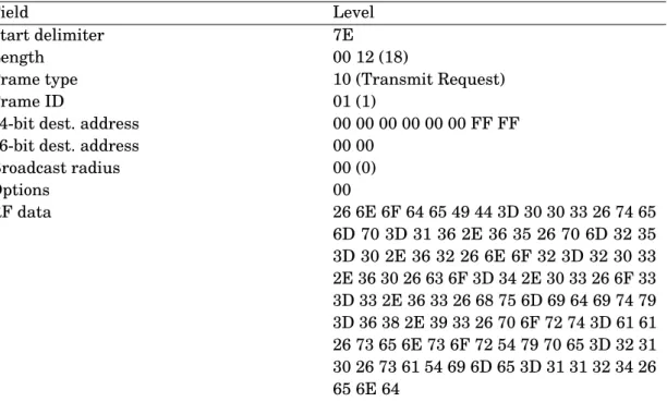
As API mode was used to interact with XBee, the 64-bit Tx frame type was used to encode the packet. For instance, a sample packet &nodeID=003&temp=16.65&pm25=0.62&no2=203.60&co =4.03&o3=3.63&humidity=68.93&port=aa&sensorType=210&saTime=1124&end, embedded in a transmission is shown in Table 3.2.
3.3 Gateway
Gateway was an Arduino[15] compatible single board computer called pcDuino[5] running Lubuntu. It was equipped with long range XBee radio and was wired by Ethernet for internet connectivity. Radio module attached here is the only designated base station radio. Gateway routine monitored the serial port for incoming packets. As the XBee was configured in API mode,
CHAPTER 3. METHODOLOGY
Field Level
Start delimiter 7E
Length 00 12 (18)
Frame type 10 (Transmit Request)
Frame ID 01 (1)
64-bit dest. address 00 00 00 00 00 00 FF FF 16-bit dest. address 00 00
Broadcast radius 00 (0) Options 00 RF data 26 6E 6F 64 65 49 44 3D 30 30 33 26 74 65 6D 70 3D 31 36 2E 36 35 26 70 6D 32 35 3D 30 2E 36 32 26 6E 6F 32 3D 32 30 33 2E 36 30 26 63 6F 3D 34 2E 30 33 26 6F 33 3D 33 2E 36 33 26 68 75 6D 69 64 69 74 79 3D 36 38 2E 39 33 26 70 6F 72 74 3D 61 61 26 73 65 6E 73 6F 72 54 79 70 65 3D 32 31 30 26 73 61 54 69 6D 65 3D 31 31 32 34 26 65 6E 64
Table 3.2: Transmission Packet
the routine was also responsible for disassembling the API frames, and to parse the data part. The data part contained the readings in name value pair fashion. Furthermore, the routine time stamped the data packet before it pushed to the cloud endpoint. A Python[40] based listener program was written to read, parse the radio packets, and push it to the cloud endpoint.
3.4 Cloud et. al.
Cloud endpoint was responsible to parse the incoming data and publish it to two interested components i.e. storage, aggregation and alerting. Figure 3.6 shows the high level components and the technology in use. TerraView™[20], a platform to store, view, analyze and control IoT data, is used as the cloud platform. There are two main components on the TerraView™side, which are MQTT broker and the Web UI. Following features were added as part of this thesis (a) Export to JSON format, (b) Publishing the message packet to store in InfluxDB - open-source distributed time series database. InfluxDB was used to generate the metrics.
3.4.1 MQTT Broker
Cloud endpoint receives the air quality packets which was pushed by the gateway, a copy is written to its database, and then it publishes to interested parties after validating. Interested parties in this case is the statistical data analyzer(via InfluxDB), Alerters, and Verifier.
3.5. SENSOR DATA PROCESSING AND ANALYSIS
FIGURE3.6. Solution Setup.
3.4.2 Web UI
Web UI showed the raw data, and gave an operational view of the system deployment. It features a 24 hrs view of all the nodes, and interactive charting feature. A dashboard with combination of plots was used to analyze the trends in the data.
3.5 Sensor Data Processing and Analysis
Cloud received 57 message packets an hour(3 AQ Nodes sending 19 packets an hour), and reading were written as they came in. No correction of data was done except in one particular scenario with NO2, the sensor gave ’INF’ readings exceeding range which was zeroed out manually
on the cloud side. It is evident in the time series plots of readings. Each node sends 6 sensor values namely NO2, PM, CO, O3, Temperature, Humidity along with ’satime’ (Number of
microseconds since the program started) and sensed timestamp. Each sensor value is stored individually after parsing with the arrived timestamp, the original packet is then discarded. The calibration was carried out on the cloud retroactively by doing the field calibration[12].
Sensor data was analyzed using TerraView™, InfluxDB and statistical software R[49]. The analysis carried out included 1-hr/8-hr means, hourly packet arrivals and correlation checks.
CHAPTER 3. METHODOLOGY
FIGURE3.7. Typical Traffic. Courtesy Google Maps
Routines were written to parse the JSON from TerraView™, and converting to CSV for R processing.
3.6 Traffic Data
Typical traffic data for the day of the week was collected from Google Maps. Google maps gives interactive visualization of traffic based on the historical traffic conditions. Traffic information is available from 6 AM to 10 PM. It is represented in four colors viz. green, orange, red, and magenta. Colors signify the condition of the traffic from fluid to stop-n-go. For analysis, historic traffic conditions were recorded in database in a form of a tuple (location, day, time, color). Location would refer to our AQ Nodes, namely Kungsgatan, Vaksalagatan and Stadsteater.
Traffic conditions are varied by nature. Figure 3.7 shows typical traffic condition on Thursday 9:35 AM along the two streets of our interest, the blue stars signify our AQ Nodes. Traffic along Kungsgatan, across from Stadsteater it is green, orange in front of Stadsteater, and magenta along Vaksalagatan. The figure gives visual confirmation of the varied nature of the traffic, and supports our placement of AQ Nodes.
C
HA
PTER
4
R
ESULTS ANDD
ISCUSSIONT
he AQ nodes were setup in month of October 2015, and were stable for more than couple of months. The system has logged more than 1000 operational hours with more than a million data points. The in-depth study is done for two weeks from last week October 2015 to first week of November 2015, unless otherwise stated.4.1 Research Questions
4.1.1 Operational Performance and Reliability
To evaluate the performance of WAQEMS, we first look at the packet deliveries, we use Packet Delivery Ratio(PDR), given by the formula � number of packets received / � number of packets sent. For the Stadshuset network, we achieved 92%, 71% respectively, and for the Stadsteater network, the ratio came to 84%. We look into packet deliveries of three nodes, we look at deliveries made per hour, with a packet arriving every 3 minutes, we expect 19 packets in an hour. There is no retransmit feature encoded into the nodes, the retransmit capability of the XBee mesh network is used instead. Figure 4.1 shows the packets delivered per hour for the three AQ nodes. Remember that Stadshuset has two nodes, and Stadsteater has one node. PDR is done for the entire month of November 2015.
While the overall reliability is in positive territory, the system exhibited high prevalence of duplicate packets in 2-node network, and missing packets. It is evident that in the Stadshuset network there is significant number duplicate packets, duplicate is identified by looking at the packet time and packet id. This is quite possibly because both the two nodes were configured as coordinators, coordinators in 868 MHz rebroadcast the packets blindly, and as gateway was in range of both the nodes, it received the same packet from both the nodes. In the broadcast mode,
CHAPTER 4. RESULTS AND DISCUSSION
FIGURE4.1. Packet deliveries by Hour
there are no acknowledgments sent, and no automatic retransmission in case of failure. Unicast could be an option to alleviate the duplicate packet issue when we expand to a wider network, and another alternative would be to place them in a wider area. Other prominent issue is with missing packets which is more sporadic in nature. There are pockets where in an hour the delivery is below par, and is pervasive in two-node network. This could be because of the interference caused by the nodes which are nearby, but this hypothesis needs to be validated. However, we did rule out ambient weather effect[34], correlation between packet loss and temperature was found to be not significant.
There was an issue with ceasing of transmission which alluded to saturation in the network. To circumvent it temporarily, a program trigger reset was initiated.
Next, we look at the time-series sensor log for the two weeks for three locations. Figure 4.2 shows the measurements of the critical pollutants, PM(density), temperature and humidity. The log is satisfactory despite duplicate packets, and small number of missing packets. Readings here are raw values i.e. resistance instead of calibrated values for pollutants, field-calibrated readings are used for doing AQI reporting. The NO2 and O3 showed fairly consistent readings at
all the AQ Nodes, and it shows peaking in the mornings, and having a repeatable trend, however CO generally tends to 0 for outdoors. The PM shows occasional spikes, and is plotted with log (base 10) as the reported concentration has extremes. NO2reading has peaked for certain times,
and is shown towering in Kungsgatan and Vaksalagatan. This resulted in giving ’INF’ value which was corrected to 0, hence the flat sections for both of these AQ Nodes. The PM sensor at Kungsgatan had instrumentation issue leading to default value. Next, to validate reliability of readings of AQ nodes, the correlation study was done for the three AQ Nodes. Figure 4.3 shows the correlation of the three AQ nodes for NO2and O3. O3at Kungsgatan and Vaksalagatan are in
4.1. RESEARCH QUESTIONS
(a) Kungsgatan (b) Stadsteater
(c) Vaksalagatan (d) PM - 3 Locations Figure 4.2: All sensors Three locations
agreement, and unexpected correlation between Stadsteater and other two locations. Kungsgatan and Vaksalagatan AQ Nodes are approximately 15 feet apart covering two streets, the correlation gives us confidence in our readings.
To ascertain correspondence to municipal monitoring station, study was done, and we saw positive agreement only for NOX when compared with our NO2readings. Figure 4.4 shows the
comparison. The Stockholm and Uppsala County Air Quality Management Association via [8] provided data of NO2, PM2.5and PM10. The data is sampled every 15 minutes. We compared
it with one of our 3 AQ nodes which was situated diagonally across the street at 10 meters height. First we studied the time series using the hourly average of the pollutants NO2 and
PM2.5, and then, linear regression was used to study the correlation. Only NO2and PM2.5could
be compared because of the availability. We intend to study the correlation of NO2further. To
qualify the strong correlation (r2> 65%) was used as benchmark. However, it showed consistency with respect to NO2, but, PM2.5had no such similarity. The most distinct trend is to be found
with NO2which peaks during morning hours, this could be explained with rush hour commuter
CHAPTER 4. RESULTS AND DISCUSSION
FIGURE4.3. AQ Nodes Correlation
The low agreement of correlation for PM may have been prominent because of the height of the AQ node with reference to Kommun, and potentially humidity correction. Our node was placed approximately 6 meters from the ground diagonally across the street whereas Kommun is placed 3 meters from the ground. Studies [62],[61] and [26] corroborate the fact that PM concentrations can vary in meters from the emission source. Secondly, the Kommun station has humidity compensation which yields in negative PM values. Underlying technology is another potential factor, the Kommun uses laser particle counter compared to ours which uses light scattering technique to measure particle mass concentration with 1µm or higher. However, the
system has the capability to be improved to give calibrated PM readings by switching to a different type of sensor. The goal of collecting PM measurements at various locations via a sensor network was met and one notable benefit of system like ours when choosing low-cost sensors is that density of the nodes can give more detailed picture of pollution[35]. Note that municipality data was provided with units of ug/m3for NO
2 and PM2.5.
Continuing with comparison, Figure 4.5 shows the correlation between AQ Egg and our AQ node on Kungsgatan with respect to O3. We see a strong positive correlation between AQ Egg
and our node. CO did not get compared because of it gave 0 reading for us as well as for AQ Egg, it is expected as higher levels are hazardous, and it occurs very rarely outdoors.
4.1. RESEARCH QUESTIONS
(a) NO2- 3 AQ Nodes (b) Kommun AQ Station
Figure 4.4: NOX Comparison at three locations
FIGURE4.5. AQ Node Correlation
4.1.2 Analysis to Discern Trends
For the period of measurements, AQ egg values showed overlap with our sensed values, and exhibits parity when average readings are considered. Furthermore, three stations gave us a denser network with promise of spatial resolution. We look now into AQI and diurnal patterns.
Figure 4.6 shows the heatmap of AQI, here AQI is overarching index covering pollutant NO2
and O3. Method documented in [24] is used to calculate the individual air quality index(IAQI)
which is further used to calculate the AQI. AQI is done separately for each pollutant using their corresponding IAQI instead of combining them, the intent is to show the effect of each
CHAPTER 4. RESULTS AND DISCUSSION
(a) AQI Kungsgatan NO2 (b) AQI Stadsteater NO2
(c) AQI Vaksalagatan NO2 (d) AQI Kungsgatan O3
(e) AQI Vaksalagatan O3
Figure 4.6: AQI using NO2and O3
pollutant lucidly. The areas in yellow show good air quality levels, and the orange shows the lightly polluted days. Days in red and purple signify alarming levels had been reached during that day, we infer it as mostly the byproduct high traffic along these two roads. This research has monitored pollutants which can be potentially harmful, and has shown that alarming levels were reached for O3gas. However, an independent assessment would be needed to corroborate it as it
affects public well-being.
Another study was to research the pattern of diurnal variation of these pollutants. Figure 4.7 shows 24 hrs data plotted for a week. This shows the pollutants have higher density in morning hours and evening hours, which can be attributed to the commuter traffic coming into the city and leaving the city. The patterns are dominant for O3 and NO2 but not as much for CO and
PM.
4.1. RESEARCH QUESTIONS
(a) NO2 (b) O3
(c) CO (d) PM
(e) Temperature
CHAPTER 4. RESULTS AND DISCUSSION
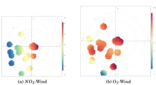
(a) NO2-Wind (b) O3-Wind
Figure 4.8: Wind - O3 and NO2 4.1.3 Ambient Weather Effects
We studied if the concentrations of these gasses had any correlation with respect to temperature and humidity. This was done with the data collected locally at the station and with the weather station data. Studies have shown the relationship between ambient weather and particulate mat-ter and crimat-teria pollutants. On the contrary, the studies have also shown that it only moderately affects the measurements[55], in this study it was inconclusive.
One of the goals we set was to confirm whether weather conditions had any influence in the readings, to carry out this study, only wind was considered[37]. The wind data was collected from the local weather station. Figure 4.8 shows wind and the AQI plotted, hourly mean values were taken of the wind speed. We found that in case of O3, for days with worse air quality, the wind
was mostly south-westerly. We do plan to investigate further into explainable models around wind and AQI.
4.1.4 Traffic Study
Traffic study was done at Stadsteater for 3 days in November - Tuesday, Wednesday and Thursday. Figure 4.9, shows the time-series of NO2, and O3in conjunction with typical traffic.
Wednesdays, and Thursdays happen to be high traffic days, and that does correlate with our derived AQI.
C
HA
PTER
5
C
ONCLUSIONSI
n conclusion, we developed and deployed an end-to-end Air Quality system in city of Uppsala. We fabricated, and installed three air quality nodes in the city of Uppsala along the two main streets Kungstatan and Vaksalagatan, with two gateways to support them. The air quality nodes measured levels of PM, CO, NO2and O3. In addition to the sensing network, twoAir Quality Eggs were collocated for comparison and calibration. The nodes performed per our expectations. The network delivered with 80% efficiency while suffering 20% packet loss, but proved to be insightful in various aspects. The measurements were also found to be comparable to the nearby official air quality monitoring unit.
There were operational concerns to begin with as Uppsala is humid and has high precipitation during the part of the year when the measurements were conducted, but the system proved to be instrumental. In the initial stages, there were issues with instrumentation, and firmware, but after few iterations, the measurements were reliably getting up to the cloud endpoint. In addition, the AQ Nodes withstood precipitation, snowfall, and ambient temperatures in the range of 18 and -4oC. However, we lost one XBee radio because of water damage caused by antenna
slot not sealed properly.
We also undertook a cloud based approach to collect, visualize, and do essential alerting. We laid a foundation to Sensor Bus lane - a highway for sensor data.
We also attested to existing work[56] that density of air quality nodes proves to counter the prevailing issue of sparseness of official monitoring stations.
Lot of enhancements would be valuable to the solution, like routine in-field calibration, over-the-air firmware update, plug-in based sensor approach(new sensors added to existing node without firmware update), and ability to switch between 868 MHz, and WiFi for network. In addition, expanding the network by installing the air quality nodes on bus stops, and data
CHAPTER 5. CONCLUSIONS
collectors on light poles would give diverse insight into pollution sources.
Another foray could be on anomaly detection; sensors are prone to multitude of faults [51], and especially gas sensors which are prone to drift [56]. Cloud infrastructure can be used to evaluate anomaly in measurements [52]. Common fault types [44] can be detected by employing methods encompassing Rule-based/Learning/Estimation/Time-series-analysis [52]. Additionally, with respect to criteria pollutant sensors, faults can be inspected real-time, and related alerting can be implemented. Also, the case of abnormal readings because of faulty calibrations can be auto-corrected using methods like blind calibration [14].
FIGUREA.1. Breakponts for AQI[24].
A
PP EN DI XA
A
PPENDIXA
B
IBLIOGRAPHY[1] Air quality egg.
http://airqualityegg.com. Accessed: 2015-07-30. [2] Digi international. http://www.digi.com. Accessed: 2015-07-30. [3] Epa pm 2.5 graphic. http://www3.epa.gov/airquality/particlepollution/graphics/pm2_5_graphic_lg. jpg. Accessed: 2015-07-30.
[4] Iceweb-principles of gas detection.
http://www.iceweb.com.au/F&g/GasDetect.htm. Accessed: 2015-08-15. [5] pcduino3. http://www.linksprite.com/?page_id=812. Accessed: 2015-08-15. [6] Seeeduino-stalker v3. http://www.seeedstudio.com/wiki/index.php?title=Seeeduino-Stalker_v3&
uselang=en, note = Accessed: 2015-09-30.
[7] Sgx sensortech. http://www.sgxsensortech.com. Accessed: 2015-09-01. [8] Slb-analys. http://slb.nu. Accessed: 2015-08-15. [9] Xbee-pro�868. http://www.digi.com/products/xbee-rf-solutions/modules/xbee-pro-868.
BIBLIOGRAPHY
Accessed: 2015-07-30.
[10] K. ABERER, S. SATHE, D. CHAKRABORTY, A. MARTINOLI, G. BARRENETXEA, B. FALT -INGS,AND L. THIELE, Opensense: open community driven sensing of environment, in
Proceedings of the ACM SIGSPATIAL International Workshop on GeoStreaming, ACM, 2010, pp. 39–42.
[11] U. S. E. P. AGENCY, National Ambient Air Quality Standards (NAAQS).
[12] R. AGRENS, Sensor Network for Real-time Air Quality Measurement, Master’s thesis,
Upp-sala University, Box 256, 751 05 UppUpp-sala, Sweden, 2015.
[13] A. AL-ALI, I. ZUALKERNAN, ANDF. ALOUL, A mobile gprs-sensors array for air pollution
monitoring, Sensors Journal, IEEE, 10 (2010), pp. 1666–1671.
[14] L. BALZANO AND R. NOWAK, Blind calibration of sensor networks, in Proceedings of the
6th international conference on Information processing in sensor networks, ACM, 2007, pp. 79–88.
[15] M. BANZI ANDM. SHILOH, Make: Getting Started with Arduino: The Open Source
Electron-ics Prototyping Platform, Maker Media, Inc., 2014.
[16] B. BISHOI, A Comparative Study of Air Quality Index Based on Factor Analysis and
US-EPA Methods for an Urban Environment, Aerosol and Air Quality Research, 9 (2009), pp. 1–17.
[17] H. BRANTLEY, G. HAGLER, E. KIMBROUGH, R. WILLIAMS, S. MUKERJEE, ANDL. NEAS,
Mobile air monitoring data-processing strategies and effects on spatial air pollution trends, Atmospheric Measurement Techniques, 7 (2014), pp. 2169–2183.
[18] S. BRIENZA, A. GALLI, G. ANASTASI,ANDP. BRUSCHI, A Cooperative Sensing System for
Air Quality Monitoring in Urban Areas, (2014), pp. 1–6.
[19] N. BULUSU ANDS. JHA, Wireless Sensor Network Systems: A Systems Perspective (Artech
House Mems and Sensors Library), Artech House Publishers Hardcove: 326 pages, 2005. [20] CALVERTVENTURESLLC, TerraView - A platform to view, analyze and control your IoT
world., Calvert Ventures LLC, California, USA, 2015.
[21] L. CAPEZZUTO, L. ABBAMONTE, S. D. VITO, E. MASSERA, F. FORMISANO, G. FATTORUSO,
G. D. FRANCIA, A. BUONANNO, E. C. R. PORTICI,ANDP. E. FERMI, A Maker Friendly
Mobile and Social Sensing Approach to Urban Air Quality Monitoring, (2014), pp. 0–4. 36
BIBLIOGRAPHY
[22] W. L. CHENG, Y. S. CHEN, J. ZHANG, T. J. LYONS, J. L. PAI,ANDS. H. CHANG, Comparison
of the Revised Air Quality Index with the PSI and AQI indices, Science of the Total Environment, 382 (2007), pp. 191–198.
[23] P. DUTTA, P. M. AOKI, N. KUMAR, A. MAINWARING, C. MYERS, W. WILLETT, AND
A. WOODRUFF, Common sense: participatory urban sensing using a network of handheld
air quality monitors, in Proceedings of the 7th ACM conference on embedded networked sensor systems, ACM, 2009, pp. 349–350.
[24] EPA OFFICE OFAIRQUALITYPLANNING ANDSTANDARDS, Guideline for reporting of daily
air quality‚Äîair quality index (AQI), Research Triangle Park, NC 27711, 1999. Guideline for reporting of daily air quality‚Äîair quality index (AQI). EPA-454/R-99-010. [25] J. FENGER, Urban air quality, Atmospheric environment, 33 (1999), pp. 4877–4900.
[26] G. GRAMOTNEV AND Z. RISTOVSKI, Experimental investigation of ultra-fine particle size
distribution near a busy road, Atmospheric Environment, 38 (2004), pp. 1767–1776. [27] J. GUTIERREZ, M. NAEVE, E. CALLAWAY, M. BOURGEOIS, V. MITTER, B. HEILE, ET AL.,
Ieee 802.15. 4: a developing standard for low-power low-cost wireless personal area networks, network, IEEE, 15 (2001), pp. 12–19.
[28] X. HAN ANDL. P. NAEHER, A review of traffic-related air pollution exposure assessment
studies in the developing world, Environment international, 32 (2006), pp. 106–120. [29] J. HAO AND L. WANG, Improving urban air quality in china: Beijing case study, Journal of
the Air & Waste Management Association, 55 (2005), pp. 1298–1305.
[30] D. HASENFRATZ, O. SAUKH, S. STURZENEGGER,ANDL. THIELE, Participatory air pollution
monitoring using smartphones, Mobile Sensing, (2012).
[31] I. HOWITT, J. GUTIERREZ,ET AL., Ieee 802.15. 4 low rate-wireless personal area network
coexistence issues, in Wireless Communications and Networking, 2003. WCNC 2003. 2003 IEEE, vol. 3, IEEE, 2003, pp. 1481–1486.
[32] D. INTERNATIONAL, XBEE-PRO 868 Range Validation, Digi White Paper.
[33] W. JIAO, G. S. W. HAGLER, R. W. WILLIAMS, R. N. SHARPE, L. WEINSTOCK,ANDJ. RICE,
Field Assessment of the Village Green Project: An Autonomous Community Air Quality Monitoring System, Environmental Science & Technology, (2015), p. 150505093732005. [34] P. A. JOHN, R. AGREN, Y.-J. CHEN, C. ROHNER,ANDE. NGAI, 868 MHz Wireless Sensor
Network - A Study, in 11th Swedish National Computer Networking Workshop, Karlstad, 2015.
BIBLIOGRAPHY
[35] M. JOVAŠEVI ´C-STOJANOVI ´C, A. BARTONOVA, D. TOPALOVI ´C, I. LAZOVI ´C, B. POKRI ´C, ANDZ. RISTOVSKI, On the use of small and cheaper sensors and devices for indicative
citizen-based monitoring of respirable particulate matter, Environmental Pollution, 206 (2015), pp. 696–704.
[36] N. KÜNZLI, R. KAISER, S. MEDINA, M. STUDNICKA, O. CHANEL, P. FILLIGER, M. HERRY,
F. HORAK, V. PUYBONNIEUX-TEXIER, P. QUÉNEL, ET AL., Public-health impact of
outdoor and traffic-related air pollution: a european assessment, The Lancet, 356 (2000), pp. 795–801.
[37] Z. LING ANDC. LEACH, The effect of relative humidity on the no 2 sensitivity of a sno 2/wo 3
heterojunction gas sensor, Sensors and Actuators B: Chemical, 102 (2004), pp. 102–106. [38] J.-H. LIU, Y.-F. CHEN, T.-S. LIN, D.-W. LAI, T.-H. WEN, C.-H. SUN, J.-Y. JUANG,AND
J.-A. JIANG, Developed urban air quality monitoring system based on wireless sensor
networks, 2011.
[39] X. LIU, S. CHENG, H. LIU, S. HU, D. ZHANG, AND H. NING, A survey on gas sensing
technology, Sensors, 12 (2012), pp. 9635–9665. [40] M. LUTZ, Programming python, vol. 8, O’Reilly, 1996.
[41] M. MASSE, REST API design rulebook, " O’Reilly Media, Inc.", 2011.
[42] R. S. MELNICK, Regulation and the courts: The case of the Clean Air Act, Brookings
Institu-tion Press, 1983.
[43] F. MURENA, Measuring air quality over large urban areas: Development and application of
an air pollution index at the urban area of Naples, Atmospheric Environment, 38 (2004), pp. 6195–6202.
[44] K. NI, N. RAMANATHAN, M. N. H. CHEHADE, L. BALZANO, S. NAIR, S. ZAHEDI,
E. KOHLER, G. POTTIE, M. HANSEN,ANDM. SRIVASTAVA, Sensor network data fault
types, ACM Transactions on Sensor Networks (TOSN), 5 (2009), p. 25. [45] W. H. ORGANIZATION ET AL., Air quality guidelines for europe, (2000).
[46] R. PIEDRAHITA, Y. XIANG, N. MASSON, J. ORTEGA, A. COLLIER, Y. JIANG, K. LI, R. P.
DICK, Q. LV, M. HANNIGAN,ANDL. SHANG, The next generation of low-cost personal
air quality sensors for quantitative exposure monitoring, Atmospheric Measurement Techniques, 7 (2014), pp. 3325–3336.
[47] C. A. POPE III, R. T. BURNETT, M. J. THUN, E. E. CALLE, D. KREWSKI, K. ITO, AND
G. D. THURSTON, Lung cancer, cardiopulmonary mortality, and long-term exposure to
fine particulate air pollution, Jama, 287 (2002), pp. 1132–1141. 38
BIBLIOGRAPHY
[48] C. A. POPE III, M. J. THUN, M. M. NAMBOODIRI, D. W. DOCKERY, J. S. EVANS, F. E.
SPEIZER,ANDC. W. HEATHJR, Particulate air pollution as a predictor of mortality in a
prospective study of us adults, American journal of respiratory and critical care medicine, 151 (1995), pp. 669–674.
[49] R DEVELOPMENTCORETEAM, R: A Language and Environment for Statistical Computing,
R Foundation for Statistical Computing, Vienna, Austria, 2008. ISBN 3-900051-07-0.
[50] B. RITZ, F. YU, S. FRUIN, G. CHAPA, G. M. SHAW,ANDJ. A. HARRIS, Ambient air pollution
and risk of birth defects in southern california, American Journal of Epidemiology, 155 (2002), pp. 17–25.
[51] A. SHARMA, L. GOLUBCHIK, AND R. GOVINDAN, On the prevalence of sensor faults in
real-world deployments, in Sensor, Mesh and Ad Hoc Communications and Networks, 2007. SECON’07. 4th Annual IEEE Communications Society Conference on, IEEE, 2007, pp. 213–222.
[52] A. B. SHARMA, L. GOLUBCHIK, ANDR. GOVINDAN, Sensor faults: Detection methods and
prevalence in real-world datasets, ACM Transactions on Sensor Networks (TOSN), 6 (2010), p. 23.
[53] S. Y. SHIN, S. CHOI, H. S. PARK,ANDW. H. KWON, Lecture notes in computer science: Packet
error rate analysis of ieee 802.15. 4 under ieee 802.11 b interference, in Wired/Wireless Internet Communications, Springer, 2005, pp. 279–288.
[54] I. SIMON, N. BÂRSAN, M. BAUER,ANDU. WEIMAR, Micromachined metal oxide gas sensors:
opportunities to improve sensor performance, Sensors and Actuators B: Chemical, 73 (2001), pp. 1–26.
[55] E. G. SNYDER, T. H. WATKINS, P. A. SOLOMON, E. D. THOMA, R. W. WILLIAMS, G. S. W.
HAGLER, D. SHELOW, D. A. HINDIN, V. J. KILARU,ANDP. W. PREUSS, The changing
paradigm of air pollution monitoring., Environmental Science & Technology, 47 (2013), pp. 11369–11377.
[56] W. TSUJITA, A. YOSHINO, H. ISHIDA, AND T. MORIIZUMI, Gas sensor network for
air-pollution monitoring, Sensors and Actuators, B: Chemical, 110 (2005), pp. 304–311. [57] P. VÖLGYESI, A. NÁDAS, X. KOUTSOUKOS,ANDA. LÉDECZI, Air Quality Monitoring with
SensorMap, (2008), pp. 529–530.
BIBLIOGRAPHY
[59] J. YICK, B. MUKHERJEE, AND D. GHOSAL, Wireless sensor network survey, Computer
networks, 52 (2008), pp. 2292–2330.
[60] P. ZAPPI, E. BALES, J. H. PARK, W. GRISWOLD,ANDT. Š. ROSING, The citisense air quality
monitoring mobile sensor node, in Proceedings of the 11th ACM/IEEE Conference on Information Processing in Sensor Networks, Beijing, China, 2012.
[61] Y. ZHU, W. C. HINDS, S. KIM, S. SHEN, ANDC. SIOUTAS, Study of ultrafine particles near
a major highway with heavy-duty diesel traffic, Atmospheric environment, 36 (2002), pp. 4323–4335.
[62] Y. ZHU, W. C. HINDS, S. KIM, AND C. SIOUTAS, Concentration and size distribution of
ultrafine particles near a major highway, Journal of the air & waste management association, 52 (2002), pp. 1032–1042.