Journal. This paper has been peer-reviewed but does not include the final
publisher proof-corrections or journal pagination.
Citation for the published paper:
Sha, Chao; Ren, Chunhui; Malekian, Reza; Wu, Min; Huang, Haiping; Ye,
Ning. (2019). A Type of Virtual Force based Energy-hole Mitigation Strategy
for Sensor Networks. IEEE Sensors Journal, p. null
URL: https://doi.org/10.1109/JSEN.2019.2945595
Publisher: IEEE
This document has been downloaded from MUEP (https://muep.mah.se) /
DIVA (https://mau.diva-portal.org).
1
Abstract—In the era of Big Data and Mobile Internet, how to
2
ensure the terminal devices (e.g., sensor nodes) work steadily for 3
a long time is one of the key issues to improve the efficiency of 4
the whole network. However, a lot of facts have shown that the 5
unattended equipments are prone to failure due to energy 6
exhaustion, physical damage and other reasons. This may result 7
in the emergence of energy-hole, seriously affecting network 8
performance and shortening its lifetime. To reduce data 9
redundancy and avoid the generation of sensing blind areas, a 10
type of Virtual Force based Energy-hole Mitigation strategy 11
(VFEM) is proposed in this paper. Firstly, the virtual force 12
(gravitation and repulsion) between nodes is introduced that 13
makes nodes distribute as uniformly as possible. Secondly, in 14
order to alleviate the "energy-hole problem", the network is 15
divided into several annuluses with the same width. Then, 16
another type of virtual force, named "virtual gravity generated 17
by annulus", is proposed to further optimize the positions of 18
nodes in each annulus. Finally, with the help of the "data 19
forwarding area", the optimal paths for data uploading can be 20
selected out, which effectively balances energy consumption of 21
nodes. Experiment results show that, VFEM has a relatively 22
good performance on postponing the generation time of 23
energy-holes as well as prolonging the network lifetime 24
compared with other typical energy-hole mitigation methods. 25
26
Index Terms—Sensor Networks, Virtual Force, Energy-hole
27
Mitigation, Path Selection, Node Position Optimization 28
29
I. INTRODUCTION 30
owadays, a large number of intelligent terminals have
31
been widely deployed in our living environment. It
32
seems that the viewpoint, "every grain of sand is a computer",
33
proposed by Mark Weiser [1] is gradually becoming a reality.
34
However, the energy issue is still an important fetter in the
35
whole Internet of Things, especially in the development of
36
Wireless Sensor Networks (WSNs). Since the battery
37
powered nodes are constrained in energy resource, it is crucial
38
to prolong the network lifetime of sensor network [2]. On the
39
Manuscript received February XX, 2019; revised XX XX, 20XX; accepted XX XX, 20XX. Date of publication XX XX, 20XX; date of current version XX XX, 20XX. This work was supported in part by the National Natural Science Foundation of P.R. China (61872194, 61872196), Jiangsu Natural Science Foundation for Excellent Young Scholar (BK20160089), Six Talent Peaks Project of Jiangsu Province (JNHB-095), “ 333 ” Project of Jiangsu Province, Qing Lan Project of Jiangsu Province, Innovation Project for Postgraduate of Jiangsu Province (SJCX18_0295) and 1311 Talents Project of Nanjing University of Posts and Telecommunications.
C. Sha, C. H. Ren, M. Wu, H. P. Huang and N. Ye are with the School of Computer Science, Software and Cyberspace Security, Nanjing University of Posts and Telecommunications, Nanjing, Jiangsu, China, 210003 (e-mail: shac@njupt.edu.cn)
R. Malekian is with the Department of Computer Science and Media Technology, Malmö University, Malmö, 20506, Sweden.
other hand, many important properties of the network such as
40
coverage, connectivity, data fidelity, and lifetime are also
41
affected by the way nodes are deployed [3-4]. In general,
42
nodes are deployed randomly or in a pre-planned manner in
43
an area called ROI (Region Of Interest). Whatever the
44
deployment method is adopted, once the network starts to run,
45
nodes may die due to hardware failures (including physical
46
damage), energy depletion, or even a small embedded
47
software bug, resulting in energy-holes [5]. The so-called
48
"energy-hole" is an area that can no longer be perceived by
49
any node (apparently, the nodes that could have monitored the
50
area are dead). In theory, the generation time and position of
51
energy-holes are often uncertain in a network with randomly
52
deployed nodes. If there are no energy replenishment, the
53
energy-holes will inevitably appear, and their scope will
54
continue to expand.
55
On the other hand, as energy consumption is exponentially
56
increased with the communication distance according to the
57
energy consumption model, multi-hop communication is
58
beneficial to data gathering for energy conservation. However,
59
such a network structure is not without problems. Since the
60
nodes close to the Sink need to forward data from other nodes
61
in the same cluster, they exhaust their energy quickly, leading
62
to an energy-hole around the Sink [6]. In this case, the
63
network will be gradually divided into more and more areas
64
that can not communicate with each other, resulting in rapid
65
failure of the entire system. Wu et al. [7] also proposed that
66
the lifetime of a uniformly deployed sensor network is mainly
67
limited by the availability of nodes around the Sink.
68
No more data can be delivered to the Sink after an
69
energy-hole appears [8-9]. In addition, nodes near these
70
energy-holes are required to bear the data load of those death
71
nodes so that the energy consumption level of them increases
72
more rapidly [10-12]. More importantly, all these phenomena
73
happen earlier than we expected. As a result, when the
74
energy-holes appear, the residual energy of most of the alive
75
nodes is relatively high. How to make full use of these nodes
76
and do everything possible to postpone the generation time of
77
energy-hole as well as to mitigate the adverse effects of it is
78
worth studying. Perillo et al. [13] first analyzed in what
79
condition the energy-holes appears. Olariu et al. [14] then
80
proved that the energy-hole inevitably appear in sensor
81
network. Many researchers regard that most of the
82
energy-holes locate around the Sink [15-16]. So, they have
83
put forward some energy-efficient routing protocols to try to
84
balance work load between nodes. Moreover, energy
85
consumption balance is also a key metrics impacting on the
86
performance of sensor network [17]. One of the most efficient
87
methods to achieve energy balance is to optimize the
88
deployment and configuration of the network. In addition, the
89
n
A Type of Virtual Force based Energy-hole
Mitigation Strategy for Sensor Networks
Chao Sha, Chunhui Ren, Reza Malekian, Senior member, IEEE, Min Wu, Haiping Huang, Member, IEEE, Ning Ye
sleep scheduling and the alternate working strategies for
1
nodes are also effective ways to postpone the generation time
2
of energy-holes and prolong the network lifetime. However, if
3
the distribution of nodes is non-uniform, the implementation
4
effect of the above strategies will be greatly reduced.
5
Therefore, "energy-hole mitigation" is in fact a multi-stage
6
collaborative optimization process.
7
II. RELATEDWORKS 8
With the advent of the era of super-large-scale ubiquitous
9
interaction, how to maximize system lifetime and balance
10
network energy consumption without human intervention has
11
become the most urgent problem in WSN. In order to alleviate
12
the energy-hole problem, scholars have carried out many
13
targeted researches from the following aspects.
14
A. Non-uniform Node Distribution on Mitigating the
15
Energy-hole Problem
16
In WSNs, the energy consumption on transmission is
17
nearly proportional to the fourth power of the hop distance,
18
when it is large. For this reason, Jia et al. proposed an optimal
19
deployment scheme for the relay nodes to solve the problem
20
of excessive energy consumption on long-distance data
21
uploading in large-scale networks [18]. Near the center of the
22
network, the node whose distance from the Sink meets certain
23
criteria was regarded as a relay. When the residual energy of
24
the edge node was lower than the threshold, it chose the most
25
suitable relay node to forward its data. Obviously, the
26
selection strategy of relay nodes directly effects the
27
generation time of energy-holes.
28
In [19], Nguyen et al. accurately calculated out the position
29
and area of the energy-hole. Then, the outer polygon of this
30
energy-hole was constructed, and the active nodes around this
31
polygon all received the message about this energy-hole. As a
32
result, data packets can be transmitted along the periphery of
33
this energy-hole, which minimizes the packet loss rate and
34
maintains the throughput of the network. However, this
35
method increases the data transmission delay.
36
A type of three-layer based network consisting of a static
37
Sink, some static sensor nodes and several proxy nodes was
38
proposed in [20]. In order to achieve energy balance, the
39
initial energy of these two types of nodes was set to different
40
values. With the help of the mobile proxy nodes deployed
41
randomly near the network center, this method effectively
42
postpones the generation time of energy-holes near the static
43
Sink. However, in areas far from the center, there were still
44
many dead nodes. With the deepening of research, people
45
gradually find that the relationship between energy-holes and
46
network coverage scheduling is more obvious. For example,
47
for a static network, its coverage often depends on how to
48
reasonably select several optimal and minimum active node
49
sets. Only the nodes in one of the active node sets need to
50
monitor the network while the rest of them can sleep, which
51
greatly reduces energy consumption of the whole network.
52
Sun et al. pointed out that as long as the node sets are
53
reasonably selected, it can ensure that the energy-holes do not
54
appear for a long time [21].
55
Furthermore, Kacimi et al. discussed the load balancing
56
techniques to mitigate energy-hole problem in large-scale
57
WSNs, and proposed a distributed heuristic solution to
58
balance energy consumption of nodes by adjusting their
59
transmission power [22]. However, it is unrealistic to
60
frequently change the data transmission power of nodes.
61
Moreover, this is also easy to increase the energy
62
consumption of nodes. While Liu et al. pointed out that the
63
deployment density of nodes in the network should be
64
inversely proportional to the distance between them and Sink
65
[23]. On the basis of this theory, they accurately calculated
66
out the First Node Die Time (FNDT) and All Nodes Die Time
67
(ANDT). This is also the basis of the network model proposed
68
by our algorithm.
69
B. Achieving Energy Consumption Balance with the help of
70
Mobile Sink
71
Recently, many studies have shown that the energy-hole
72
problem can be effectively mitigated by using one or more
73
mobile Sinks [24].
74
Zhang et al. [25] proposed an optimal cluster-based
75
strategy to achieve load balancing in data collection with the
76
help of several mobile Sinks. Moreover, the Rendezvous
77
Points (RPs) and Rendezvous Nodes (RNs) were then
78
introduced to further reduce time delay. However, the
79
network topology in this method can never be changed
80
anymore, which is often unrealistic.
81
To enhance the network coverage and minimize the sensing
82
redundancy, Sahoo et al. proposed a distributed energy-hole
83
repair method [26]. According to their locations, nodes were
84
classed into three categories, that were cross triangle node,
85
hidden cross triangle node, and non-cross triangle node.
86
Through the interaction between different types of nodes,
87
high coverage redundancy areas and energy-holes were found
88
out. Subsequently, several nodes located in the high coverage
89
redundant area were moved to the location of the
90
energy-holes to repair them. Obviously, this method can
91
reduce the probability of energy-holes to some extent by
92
adjusting the network topology, but its real-time performance
93
still needs to be improved.
94
In [27], the author tried to solve the energy-hole problem
95
by using some mobile relay nodes. The network is divided
96
into several clusters with different sizes, and each "relay
97
node" is responsible for uploading the sensing data of several
98
clusters to Sink. That is to say, the relay node is a mobile data
99
collector relative to the "sub-region" composed of several
100
clusters. This algorithm is very suitable for event-driven
101
networks or networks that need continuous data transmission.
102
With the help of these "mobile relay nodes", the energy
103
efficiency as well as load balance of the whole network have
104
been greatly improved. However, this method relies too much
105
on "relay nodes". Once these relay nodes fail or their data
106
forwarding efficiency is low, some nodes (especially the
107
cluster header nodes) will prematurely die, resulting in the
108
energy-holes.
109
Abo-zahhad et al. used the clustering mechanism combined
110
with one mobile Sink to alleviate the energy-hole problem
111
[28]. Based on the adaptive immune algorithm of energy
dissipation, they calculated the optimal number of cluster
1
heads. Then, the trajectory of the mobile Sink was also
2
obtained, which can reduce the burden of cluster heads to a
3
certain extent and postpone the generation time of
4
energy-holes. However, this method did not fundamentally
5
solved the problem of unbalanced energy consumption of
6
nodes.
7
In the era of mobile Internet, more and more scholars point
8
out that besides Sink or relay nodes, other nodes should also
9
be able to move in WSNs. They believe that after being
10
deployed, nodes can move freely to the area where the
11
energy-holes appear, so that those holes can be repaired. In
12
this case, how to select out the appropriate nodes to repair the
13
holes and how to move these nodes to the right position are
14
two critical issues. One of the feasible solutions is to use the
15
"virtual force". Adjacent nodes can exert attractive or
16
repulsive force to each other. For non-adjacent nodes, there is
17
no virtual force between them. However, most of the current
18
researches on virtual force are still in the conceptual stage. In
19
these works, the magnitudes of virtual force between nodes
20
are not quantified according to the specific network structure.
21
In this paper, the distance between nodes in specific network
22
structure is fully analyzed, and two kinds of quantification
23
models for the virtual force are described. On this basis, the
24
network topology is optimized that can mitigate the
25
energy-hole problem.
26
C. Mitigating the Energy-hole Problem in Circular Network
27
Although the shape of Wireless Sensor Network is various
28
in real scenarios, it can be abstracted as a circular network
29
whether it is a cluster based structure or a multi-hop network
30
structure. In this section, we introduce the energy-hole
31
mitigation strategies in the circular network.
32
In [29], a circular network is divided into several annuluses
33
at first, and then each annulus is divided into smaller sectors.
34
The authors proved that this logical partition method can
35
reduce the probability of energy-holes. However, this method
36
did not take into account the distance between the node and
37
cluster head in the real scene, which may result in high energy
38
consumption.
39
A type of Wireless Sensor Network Energy Hole Alleviating
40
(WSNEHA) algorithm was proposed in [30]. The network was
41
divided into several annuluses with the same width, as shown
42
in Figure 1. A static Sink was located in the center of the
43
network, and nodes were evenly distributed in each annulus.
44
For each node in the second annulus, according to the
45
real-time energy consumption rate of all its possible
46
successors, the most suitable one was selected as its
47
forwarding node. Thus, the load of each node in the innermost
48
annulus can be balanced. On this basis, Jan et al. [31] further
49
discussed the load balancing problem of nodes in each
50
annulus, and its network structure is shown in Figure 2. In this
51
model, nodes were randomly distributed in each annulus.
52
Based on distance and energy constraints, each node adopted
53
the minimum bit error rate transmission strategy to select its
54
next hop forwarder. However, neither method mentioned
55
above is flexible enough. In the case of dense deployment of
56
nodes, their effect on mitigating energy-holes is not obvious.
57
58
Fig. 1. Network model of WSNEHA [30]. 59
60
Fig. 2. Network model proposed in [31]. 61
Wu et al. [7] pointed out that in a circular network with
62
non-uniform distribution of nodes and constant data
63
uploading rate, the phenomenon of unbalanced energy
64
consumption of nodes is unavoidable. However, if the number
65
of nodes can be increased from the outer annulus to the inner
66
one layer by layer according to geometric series, the
67
energy-hole problem may be avoided to some extent. For this
68
reason, they proposed a non-uniform node deployment
69
strategy and obtained the proportional relationship between
70
the number of nodes in the adjacent annulus. However, there
71
were too many nodes deployed near the network center,
72
which easily causes a lot of coverage redundancy.
73
D. Using Energy Replenishment Technology to Prevent the
74
Appearance of Energy-holes
75
All the methods mentioned above can not fundamentally
76
eliminate the energy-hole, and they can only postpone the
77
time it appears. In recent years, the continuous improvement
78
of Wireless Energy Transfer (WET) technology has made it
79
possible to replenish energy to the ubiquitous sensor nodes by
80
a non-contact way, that is, Wireless Rechargeable Sensor
81
Networks (WRSNs). For most of the energy replenishment
82
strategies, one or more Mobile Wireless Charger (MWC) are
83
often employed to periodically recharge all nodes along some
84
fixed trajectories, or they only recharge the nodes on demand
85
when randomly walking. In this way, as long as the nodes are
86
able to be charged in time before death, the energy-hole can
87
be eliminated theoretically.
88
Wang et al. [32] divided the network into annuluses to
89
alleviate the “energy-hole problem”. The recharging
90
threshold was set for each node depending on its energy
91
consumption rate and the length of the request queue, which is
92
more reasonable for large-scale networks. Moreover, the
93
recharging order of nodes was obtained by constructing a
94
Minimum cost Spanning Tree (MST) covering all nodes in
95
the recharging request queue. In this way, they can achieve a
relatively high recharging profit. However, the recharging
1
threshold in all these preceding works was mainly determined
2
by node’s energy, which failed to intuitively reflect the
3
residual lifetime of a node.
4
Zhu et al. [33] strictly limited the battery capacity of WCV
5
and proposed a type of Node Failure Avoidance Online
6
Charging scheme (NFAOC) based on node’s real-time energy
7
consumption rate. Nodes which cause the smallest number of
8
dead nodes is selected as the next recharging object, thereby
9
assuring high recharging efficiency. It should be pointed out
10
that this strategy tends to fall into local optimum during the
11
path construction phase, which reduces the number of nodes it
12
can serve. Therefore, it can not completely eliminate the
13
energy-hole.
14
In order to make MWC charge more nodes in a limited time,
15
Xu et al. [2] assumed that the actual energy required by the
16
node should be evenly replenished during multiple recharging
17
rounds. That is to say, only a part of energy need to be
18
replenished to node each time. Although this method
19
increases the number of nodes that a MWC can serve, it also
20
accelerates the scheduling frequency as well the energy
21
consumption rate of the MWC.
22
Although WRSN plays a positive role in alleviating the
23
energy-hole problem, it is also undeniable that the cost of the
24
wireless mobile charger is relatively higher and the
25
scheduling algorithm is a little complex. In addition, the
26
moving speed as well as the charging efficiency of WMC are
27
low. All these factors make it impossible for such methods to
28
completely prevent the generation of energy-holes.
29
On the basis of the above researches, we propose an
30
energy-hole mitigation strategy with the help of two kinds of
31
virtual force. Contributions of this paper can be concluded as
32
follows.
33
Firstly, under the action of virtual gravitation and repulsion
34
force, nodes are uniformly distributed in the network which
35
ensures that no blind area of perception appear during a long
36
time.
37
Secondly, position of each node is further optimized with
38
the help of the "virtual gravity generated by annulus". This
39
not only reduces the load of nodes near the center but also
40
ensures the coverage of the whole network.
41
Finally, nodes are classified into two categories, which are
42
responsible for sensing and data forwarding, respectively.
43
The optimal number of each kind of nodes located in each
44
annulus and the weights of all possible data uploading paths
45
in the "data forwarding area" are calculated out for path
46
selection. This further balance energy consumption on data
47
uploading.
48
The remainder of this paper is organized as follows. The
49
related works are described in section II. And the network
50
model as well as the virtual force based energy-hole
51
mitigation method are described in section III. Experimental
52
results of VFEM are shown in section IV and the conclusion
53
is provided in the last section.
54
III. METHOD DESCRIPTION
55
A. Network Model
56
It is assumed that N sensor nodes are randomly deployed in
57
a circular region whose radius is R. The base station B is
58
located at the center of network. According to [7], both the
59
maximum communication radius and maximum sensing
60
radius of each node are the same (the value of them is defined
61
as r). The initial topology after deployment is shown in Figure
62
3, in which the sensing data can be sent to the base station via
63
one-hop or multi-hop transmission.
64
65
Fig. 3. Nodes are randomly deployed in the circular network. 66
Without loss of generality, the energy dissipation model
67
adopted by VFEM is the same as that in [7] and [34], as
68
shown in Figure 4.
69
70
Fig. 4. Energy dissipation model [30]. 71
In formula (1) and (2), Esend and Erec are the energy 72
consumption of one node during its sending and receiving
73
phase. Eelecis the unit energy consumption of the circuit. εfsand 74
εamp are the signal amplifier in the free space and multi-path 75
fading environment, while d'= e efs amp denotes the threshold 76
distance.
77
To transmit a c-bit message a distance d, the radio expends
78 2 4 ' ( , ) ' elec fs send elec amp cE c d d d E c d cE c d d d e e ì + < ï = í + ³ ïî (1) 79
And to receive this message, the radio expends
80
( )
rec elec
E
c
=
cE
(2)81
B. Node Position Adjustment Based on Virtual Force
82
between Sensors
83
Generally speaking, random deployment is easy to realize
84
in sensor network. However, uneven distribution of nodes in
85
the network could easily cause data redundancy and
86
perceptual holes. On the other hand, the long hop distance
87
between nodes may cause unbalanced energy consumption on
88
communication, and this also shorten the network lifetime.
Thus, the primary goal of VFEM is to make nodes distribute
1
as uniformly as possible.
2
According to [28], if sensor nodes can be finally deployed
3
as the structure shown in figure 5, the network is regarded as
4
to achieve a nearly uniform distribution. The black dots are
5
the ideal positions of nodes, while the hexagon in this figure is
6
the actual sensing region of each node when no coverage hole
7
appears. We can see that the area composed by all the regular
8
hexagons cover the whole network. In this case, the density of
9
nodes (defined as ρ) is 2
2 3 3l [28]. l is the length of each
10
regular hexagon and it is not difficult to know that,
11
(
)
2 3 3 1 l=p
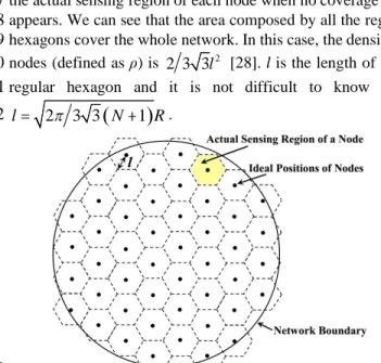
N+ R. 12 13Fig. 5. Nodes are uniformly deployed in the circular network. 14
Nowadays, people have made a lot of efforts on improving
15
both the distribution of nodes in network and optimizing the
16
network topology [7, 13]. Node’s position adjustment with
17
the help of virtual force is one of the effective strategies. The
18
concept of virtual force was first proposed in path planning
19
and barrier avoidance for robots. Then, it was introduced to
20
Wireless Sensor Networks to try to solve the coverage
21
enhancement problem. The basic idea of virtual force is to
22
assume each node as charge so that it will obtain virtual force
23
from other nodes. With the effect of this virtual force, nodes
24
may move to other positions and finally achieve equilibrium
25
on force which ensures full coverage of the network.
26
Thus, in VFEM, it is regarded that one node has virtual force
27
(gravitation and repulsion) with another one when the distance
28
between them meets certain constraints. With the help of these
29
virtual force, nodes can move within the network (there is
30
friction between node and ground) and finally reach to a
31
stationary state in which the distance between two adjacent
32
nodes is nearly equal to l. Here, we take two sensor nodes (Si 33
and Sj) as an example to describe the definition of virtual force 34
in VFEM.
35
1) When
0
3l-d £dij£ 3l, it is assumed that, there is no
36
force between Si and Sj. dij is the Euclidean distance 37
between Si and Sj. Moreover, to avoid nodes’ repeated 38
movement that is caused by virtual force, d0is introduced 39
as the buffering distance and d0Î
(
0,3 2l)
.40
2) If dij< 3l-d0, it is obvious that, the distance between Si 41
and Sj is short. To make the nodes approach the state of 42
uniform distribution as shown in Figure 5, Siand Sjneed to 43
get away from each other. Thus, there is only repulsion
44
force between Siand Sjin this case, and the value of this 45
force is η/dijβ. η is defined as the coefficient of this repulsion 46
and β is an adjustable parameter. Values of η and β are
47
described in the experimental section.
48
3) When 3l<dij<2 3l-d0, the distance between Siand Sj 49
could be considered a little long. Similarly, to make the
50
nodes approach the state of uniform distribution, Siand Sj 51
need to get close to each other. Therefore, there is only
52
gravitation force between Si and Sj in this case, and the 53
value of this it is set to λdijβ. λ is the coefficient of this 54
gravitation.
55
4) If 2 3
ij
d ³ l, it is known that, the distance between Siand 56
Sjis too long. So, there is no force between these two 57
nodes.
58
We use Fji to mark the virtual force from Sj to Si. In 59
summary, we can get
60 0 0 0 3 3 2 3 0 3 3 2 3 ij ij ji ij ij ij ij d d l d F d l d l d l d d l or d l b b h l ì < -ï ï =í < < -ï ï - < £ ³ î (3) 61
It is worth mentioning that, the base station is regarded as a
62
common sensor node, and it generates repulsion and gravitation
63
to other nodes. However, to ensure that the location of B does not
64
get change, we assume that the base station is not acted upon by
65
the virtual force generated by other nodes.
66
What’s more, to avoid nodes moving out of the network,
67
the network boundary exists repulsive force to Si(marked as 68
Fbi) in a certain range. The direction of Fbipoints to the center 69
of network and the value of it is defined as follows.
70
(
)
(
)
(
)
(
)
, 0 , 0 , i i bi i d b S d b S l F d b S l t h ì £ £ D ï = í ï > D î (4) 71In formula (4), d(b,Si) is the shortest distance between Si 72
and the network boundary. Thus, d(b,Si)=R-d(B,Si). (d(B,Si) is 73
the Euclidean distance between base station B and node Si). In 74
addition, Δl is an adjustable distance, and Δl<<l.
75
Moreover, from the above analysis, it is easy to know that,
76
the minimum gravitation and repulsion force between two
77
nodes are l
(
3l)
b and(
3l d0)
bh - , respectively. The
78
minimum repulsion force generated from the network
79
boundary to the node is η/(Δl)τ. Therefore, to make the nodes
80
approach the state of uniform distribution, the friction f ought
81
to be smaller than the minimum value of virtual force. That is,
82
(
)
(
)
( )
(
3 , 3 0 ,)
f <Min l l b h l-d b h Dl t (5) 83
Thus, the resultant force acting on Sicould be expressed as 84 follows. 85
(
)
1, N i ji bi j j i F S F F f = ¹ =å
+ +uuuuuur uur uur ur
(6)
86
So, when the sensor node is deployed in the network, it moves
87
along the direction of the resultant force until the value ofF S
( )
i uuuuuur88
is equal to zero and will not change any more.
C. Optimum Number of Nodes in Each Annulus
1
Although the uniform distributed nodes can ensure that no
2
perceptual blind area appears for a long time, when radius of
3
the network is too big, nodes have no choice but to transmit
4
data to the base station with multi-hop transmission manner.
5
In this case, it will increase the load of the nodes near the
6
center. To relieve the "energy-hole problem", the "virtual
7
gravity generated by annulus" is proposed to further optimize
8
the positions of nodes.
9
Similar to Wu [7] and our previous work [35], in VFEM,
10
the circular network is divided into k annular regions with the
11
same width (marked as dw), as shown in Figure 6. The annular 12
regions from inside to outside are marked as C0, C1…Ck-1. 13
Actually, C0 is a circle whose radius is dw. As mentioned 14
above, nodes near the center may bear more data transmission
15
tasks. So, it is a good choice to allocate different number of
16
nodes in different annular regions to balance energy
17
consumption. However, this may increase the coverage
18
redundancy and the efficiency on data collection may also be
19
reduced. On the other hand, in most data collection and
20
routing methods, nodes are often regarded to be "fully
21
functional", that is, they can act as sensing terminals, relay
22
nodes, or even cluster heads. Nevertheless, the difference on
23
energy consumption between nodes may become larger and
24
larger in this way. Therefore, it is assumed that there are two
25
kinds of nodes exist in the network.
26
Sensing Nodes: These nodes (the white dots in Figure 6)
27
only do the sensing and data uploading tasks, and they can not
28
receive data form other nodes.
29
Relay Nodes: This type of nodes (the grey dots in Figure 6)
30
only receive data sending from nodes in the adjacent outer
31
annulus. Then, they forward these data to the relay nodes
32
located at the adjacent inner annulus so that all the sensing
33
data can finally be transmitted to the base station. It is worth
34
noting that, relay nodes can not perceive information.
35
36
Fig. 6. Network model of VFEM. 37
Moreover, to further enhance the efficiency on sensing and
38
to facilitate the relay nodes finding out the optimal data
39
uploading paths, nodes in the same annulus should be located
40
at the center of this annulus (the dotted line in Figure 6). In
41
this case, the shortest distance from the node to both the outer
42
and inner side of the annulus is dw/2. 43
It is assumed that, in a round of data collection time, each
44
sensing node gets c bits data and forwards them to the
45
next-hop node until to the base station. To avoid the
46
"energy-hole problem", energy consumption rate of each
47
node should be roughly the same with each other. That is,
48
E0′/E0≈E1′/E1≈...Em′/Em...≈Ek-1′/Ek-1. Em′ is defined as the total 49
energy consumption of nodes in Cmduring a round of data 50
gathering time, while Emis the sum of initial energy of all the 51
nodes in Cm. It is also assumed that, Nmsand Nmrrepresent the 52
number of sensing nodes and relay nodes in Cm, respectively. 53 Thus, 54
(
)
(
)
(
)
(
)
(
)
(
)
1 2 1 1 0 1 2 2 0 1 1 2 1 1 0 1 0 1 0 0 0...
'
'
k s s s t k t r i k i t k s s r k k k k s s t t r i i s r k s s t t r i i s r
e N
e
e
N
e N
e N
N
N
e
e N
e
e
N
N
N e
e N
e
e
N
N
N e
-- = -- - -= -=+
+
»
»
+
+
+
»
+
+
+
»
+
å
å
å
(7) 55In formula (7), e0represents the initial energy of each node. 56
etand et′ are the transmission energy consumption of nodes in 57
Cm(m>0) and C0respectively during a round of data collection 58
time. eris the energy consumption on data receiving. That is to 59 say, 60 2 t elec fs
e
=
cE
+
c
e
d
(8) 61(
)
2'
2
t elec fs we
=
cE
+
c
e
d
(9) 62 r elece
=
cE
(10) 63It is necessary to point out that, the parameter d in formula
64
(8) is defined as the expected value of distance between a pair
65
of transmitting and receiving nodes located in adjacent
66
annuluses. The value of it is discussed in the following section.
67
As mentioned before, nodes in C0only need to send data to 68
the base station, so the distance about the last hop is dw/2. 69
From the above analysis, it is known that, the number of the
70
sensing and relay nodes in each annulus are critical for
71
balance of energy consumption. Therefore, the values of Nms 72
and Nmrare discussed as follows. 73
To enhance the efficiency on data collection, sensing nodes
74
should meet the following conditions.
75
1) The sum of sensing regions of all these nodes should
76
cover the whole network. That is to say, there is no blind area
77
on sensing.
78
2) Each sensing node should be able to upload data to at
79
least one relay node in the adjacent inner annulus.
80
3) The proportion of overlapping coverage area in the
81
network should be as small as possible.
82
In order to meet condition 1) and 2), both the sensing radius
83
and communication radius are set to 1.5dw. Meanwhile, to reduce 84
the redundancy on data collection, nodes in each annulus should
85
be uniformly distributed. Moreover, area of the overlapping
86
sensing region should be as small as possible, as shown in Figure
87
7. The red dashed lines in Figure 7 are the perception boundaries
88
of each sensing node in Cm. 89
According to cosine theorem, the relationship between the
90
three sides of△ABC in Figure 7 can be expressed as follows.
(
)
(
(
)
)
(
(
)
)
(
)(
)
2 2 2 2 1.5 0.5 1 2 0.5 1 cos w w w w d m d m d m m da
= + + + - + + (11) 1 Thus, 2(
) (
)
(
2 2)
arccos 2 3 1 2 3 1 s m N m m m mp
é ù ê ú = ê ú + - + + ê ú ê ú (12) 3And the value of Nmrcould also be solved out by formula (7) 4 and (12). 5
(
)
[
]
(
)
1 1 1 11
1,
2
1
'
0
k s r t i m i r m k s r t i ie e
N
m
k
N
e e
N
m
-= + -=ìé
+
ù
Î
-ê
ú
ïê
ú
= í
é
ù
ï
ê
+
ú
=
ê
ú
î
å
å
(13) 6 That is, 7[
]
1 1 2 1 1 2 1 1, 2 4 1 0 4 k s elec i i m elec fs r m k s elec i i elec fs w E N m k E d N E N m E de
e
-= + -= ìéæ ö ù ïêç + ÷ ú Î -ïêç + ÷ ú è ø ïê ú = í éæ ö ù ï êç ÷ ú ï + = êç ÷ ú ï + è ø ê ú îå
å
(14) 8 9Fig. 7. Deployment of nodes with no energy-holes. 10
On the other hand, for the sensing node in Cm(m>0), the 11
shortest and longest distance from this node to its next-hop
12
successor are dwand 1.5dwrespectively. As shown in Figure 7, 13
the next-hop successor of node A (e.g., node D) can only be
14
located at one position on curve ab. The angle value of
15
∠ABD is set to iα/n(i≤n). Thus, by using the cosine theorem,
16
it is easy to know the distance of segment AD, and the length
17
of the single hop distance could also be calculated out by
18 formula (15). 19
(
)
(
)
(
(
)
)
(
)(
)
(
)
2 2 2 1 0.5 0.5 1 lim 2 0.5 0.5 cos n w w n i w m d m d d n m m d ia n ®¥ = æ ö + + -ç ÷ = ç ÷ ç - + - ÷ è øå
(15) 20It is known from formula (12) that, in formula (15),
21
(
)
(
)
(
2 2)
arccos 2m 3m 1 2m 3m 1a
= + - + + (16) 22D. Nodes’ Positions Optimization based on Virtual Force
23
Generated from Annulus
24
As mentioned earlier, only if the number of the sensing and
25
relay nodes in Cmare equal to Nmsand Nmrrespectively, energy 26
consumption of them are nearly the same with each other. Thus,
27
we assume that the curve located in the middle of each annulus
28
(e.g., Cm) can also generate virtual force (marked as F C
(
m)
uuuuuuur
) so
29
that corresponding number of nodes will finally move onto
30
each curve. The final distribution of nodes is shown in Figure 6.
31
Sphere of influence from this virtual force generated by
32
curve in Cm(m>0) is also an annular region whose center is 33
the base station. The inner and outer boundaries of these
34
regions are drawn with the red solid lines in Figure 8, and the
35
width of each region is marked as dF(Cm). So, lengths of the 36
inner and outer diameters of Cm are
( )
1 0 2
å
m=- F i i d C and 37( )
02
å
im= dF Ci , respectively. The influenced area of the 38virtual force generated by the curve located in the middle of
39
C0is a circle whose radius is dF(C0). 40
As mentioned in Section III.B, all nodes have been nearly
41
uniformly distributed in the network with the action of the
42
virtual force between nodes. Now, the virtual force generated
43
by annulus only needs to keep the number of nodes in the
44
sphere of influence approximately equals to Nms+Nmt. That is, 45
(
)
(
)
(
)
2 2 0 0 m m s t F m j j i j d C N R N N p p = = æ ö = + ç ÷ ç ÷ èå
øå
(17) 46 So, 47( )
(
2)
(
)
0 0 = m m s t F m j j i j d C R N N N = = +å
å
(18) 48The value of dF(Cm) can be calculated out by mathematical 49
induction.
50
51
Fig. 8. Virtual force generated from annulus. 52
Due to this kind of virtual force, nodes move onto the curve
53
located in the middle of each annulus. Take Siin Figure 8 as an 54
example. The white dot formed by the dotted line is the
55
position of Siafter the action of the first kind of virtual force. 56
We can see that this position is in the scope of influence of the
57
virtual force generated by the dotted curve in Cm. Hence, Si 58
further moves to the position of the white dot formed by the
59
solid line.
60
Moreover, if nodes are uniformly distributed on the circular
61
arc, the minimum redundancy can be guaranteed. Therefore,
62
position of sensing nodes should be further improved. That is,
63
for two adjacent sensing nodes ( e.g., Si and Sj) in Cm, the 64
value of∠SiBSjshould be 2π/Nms, as the white nodes shown 65
in Figure 6.
In addition, from formula (13), it is not difficult to know
1
that, the number of the sensing nodes located in Cm+1(m>0) 2
and C1satisfy the following constraints. 3
(
)
( )(
)
max 1 Num R avg j jT
TP
t
Num R
=D
=
å
D
(19) 4(
)
1 11
'
1 0 k s s r r t i iN
<
é
ê
ê
+
e e
å
=-N
ù
ú
ú
=
N
(20) 5So, the number of the relay nodes in Cm(k-1>m≥0) must be 6
larger than that of sensing nodes in Cm+1. Thus, these relay 7
nodes should also be uniformly distributed on the curve, as
8
the gray nodes shown in Figure 6. This ensures that each
9
sensing node is able to find out at least one relay node as its
10
next-hop successor, as shown in Figure 7. Sensing nodes in C0 11
straightly send data to the base station without forwarding.
12
Similarly, it is also known from formula (13) that, the
13
number of relay nodes in Cm(k-2>m≥0) is larger than that of 14
relay nodes in Cm+1. That means when the relay nodes are 15
uniformly distributed on each curve, each relay node in Cm+1 16
can certainly find out at least one relay node in Cm as its 17
next-hop successor.
18
Furthermore, with the help of formula (12) and (13), it can
19
also be concluded that, when m is smaller, the value of Nms 20
will be smaller too while the value of Nmrwill be larger. That 21
is, the closer to the base station, the less the number of sensing
22
nodes, but the more the number of relay nodes. In this way,
23
each node has more choices to select the optimal next-hop
24
successor, and the “hotspot problem” can also be alleviated to
25
a certain extent. It is helpful to postpone the generation time
26
of energy-holes.
27
E. Optimal Path for Data Uploading
28
Now, each node has moved onto the middle position of
29
each annulus with the help of the virtual force generated from
30
annulus, as shown in Figure 6. Meanwhile, all the sensing and
31
relay nodes have been uniformly distributed on the curve.
32
Although it is proved that, each node can find out at least one
33
successor for data uploading, if there is no limitation on path
34
selection, the hop distance might be long. As shown in Figure
35
9, the length of each hop is close to or equal to 1.5dw. This not 36
only increases the energy consumption on communication,
37
but also aggravates the burden on some relay nodes (e.g.,
38
node Si). 39
40
Fig. 9. Unreasonable data uploading paths. 41
Therefore, the concept of “data forwarding area” is
42
proposed here. As we know, the boundary of sensing range of
43
node Si in Cm (k>m>0) will intersect with the curve in the 44
middle of Cm-1at two points, such as point a and b in Figure 7. 45
The sector area formed by arc ab, line segment aB and line
46
segment bB is defined as the "data forwarding area" (the
47
sector region in Figure 10). For any sensing node Sj, the 48
next-hop successor of it can only be selected out from the
49
"data forwarding area".
50
51
Fig. 10. Data forwarding area. 52
For one sensing node (e.g., Si) in Cm+1 (k-1>m>0), it is 53
assumed that Sj(located at Cj) and S0(located at C0) are two 54
candidate relay nodes of Siin the "data forwarding area". Thus, 55
"Si→Sj→Sj-1→…→S0→B" can be regarded as one of the 56
possible data uploading paths (marked as pathi). The weight 57
of pathiis defined as follows. 58
(
)
1(
)
2(
)
(
)
2(
)
1 0 0 , , i r j j j r j m W path E S d S S- E S d S B = =å
+ (21) 59In formula (21), Er(Sj) is the residual energy of Sj. d(Sj,Sj-1) 60
is the Euclidean distance between Sjand Sj-1while d(S0,B) is 61
the Euclidean distance between S0 and the base station. 62
Sensing node Sicalculates out all the possible paths’ weights 63
with the help of formula (21), and it then selects out the path
64
with the largest value of weight as the data uploading path
65
(the blue arrow in Figure 11).
66
67
Fig. 11. The optimal data uploading path. 68
Both the residual energy of the relay nodes in "data
69
forwarding area" and the hop distance between nodes are
70
considered in selecting out the optimal data uploading path.
71
For this reason, VFEM can ensure energy consumption
72
balance to a certain extent. However, it is possible for some
sensing nodes to choose the same relay node as the successor
1
in their uploading paths, which greatly increases the energy
2
consumption on some relay nodes (e.g., node S2in Figure 12). 3
In order to solve this problem, each sensing node should
4
monitor the residual energy of all the forwarding nodes in its
5
"data forwarding area" at the end of each round of data
6
uploading. When the residual energy of Sj is lower than its 7
threshold Eror the standard deviation for all the relay nodes in 8
the "data forwarding area" is higher than the threshold δ
9
(definition of δ is shown in formula (22) ), Sjwill select out 10
another data uploading path according to formula (21).
11
Meanwhile, these relay nodes whose residual energy is lower
12
than Erare regard as dead nodes. 13
(
)
(
)
(
)
( )(
)
(
)
( )(
)
2 2 1 1 i i Num S Num S r k r k k k r k i i E S E S D E S Num S Num S = = æ ö ç ÷ ç ÷ = - ç ÷ ç ÷ ç ÷ è øå
å
(22) 14In formula (22), Num(Si) is the total number of relay nodes 15
in the “data forwarding area”.
16
17
Fig. 12. Loads on the relay nodes. 18
It is worth mentioning that, in VFEM, the
19
computation complexity on path selection is not high. Take a
20
circular network which is divided into 5 virtual annuluses as
21
an example, it is not difficult to know that, the number of
22
sensing nodes in C4, C3, C2, C1and C0are 11, 9, 7, 4 and 1. 23
While the number of relay nodes in C3, C2, C1 and C0are 24
⌈11(1+er/et)⌉, ⌈20(1+er/et)⌉, ⌈27(1+er/et)⌉ and ⌈31(1+er/et)⌉, 25
respectively. Due to the fact that the sensing and relay nodes
26
are uniformly distributed in each curve, there won't be too
27
many relay nodes in each "data forwarding area". For
28
example, for any sensing node in C4, the total number of relay 29
nodes in its "data forwarding area" is only⌈11(1+er/et)/11⌉+ 30
⌈20(1+er/et)/11⌉+⌈27(1+er/et)/11⌉+⌈31(1+er/et)/11⌉. Thus, 31
the there are at most ⌈(20×27×31/113)(1+e
r/et)4⌉ possible 32
paths for selection. It is known from [30] that, eris far less 33
than et, so the number of the possible paths for data uploading 34
is only about 13. Thus, computation cost on the optimal path
35
selection algorithm in VFEM is low.
36 37
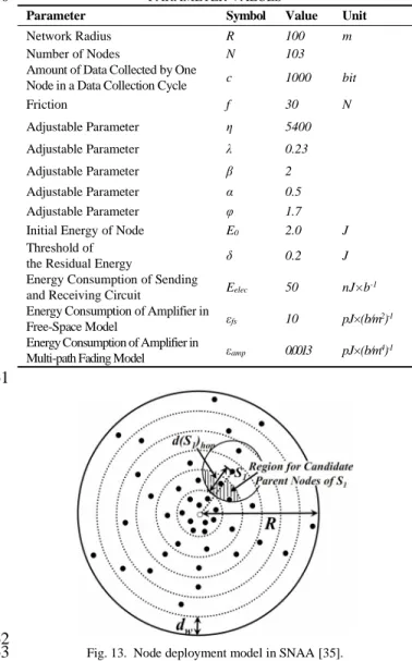
IV. SIMULATION RESULTS AND ANALYSIS
38
Simulation results are carried out with the help of Matlab
39
8.5. All the experiments were carried on a server (the
40
operating system is Win 10) with Intel Xeon (E3-1225V6)
41
3.3GHz CPU, 16GB memory(DDR4, 2400MHZ), 8MB
42
cache and 2TB hard disk. All the algorithms were
43
implemented via Java code. We compare VFEM with SNAA
44
[35] (an energy-hole mitigation strategy proposed by our
45
previous work) and the method proposed by Wu [7]. In
46
SNAA, the circular network is also divided into virtual
47
annuluses with the same width. Nodes are non-uniformly
48
deployed, and the number of them increases in geometric
49
progression from the outer annuluses to the inner ones, which
50
effectively reduces the work load on nodes near the center.
51
Moreover, each node can find its optimal parent by
52
considering the residual energy of each candidate as well as
53
the distance between the two nodes in adjacent annuluses. The
54
node deployment model and the data uploading process in
55
SNAA are shown in Figure 13 and 14. Values of the
56
experimental parameters are shown in Table I. All the data of
57
each experiment were obtained after 100 times of simulations.
58
TABLE I 59
PARAMETER VALUES 60
Parameter Symbol Value Unit
Network Radius R 100 m
Number of Nodes N 103
Amount of Data Collected by One
Node in a Data Collection Cycle c 1000 bit
Friction f 30 N Adjustable Parameter η 5400 Adjustable Parameter λ 0.23 Adjustable Parameter β 2 Adjustable Parameter α 0.5 Adjustable Parameter φ 1.7
Initial Energy of Node E0 2.0 J
Threshold of
the Residual Energy δ 0.2 J
Energy Consumption of Sending
and Receiving Circuit Eelec 50 nJ×b
-1
Energy Consumption of Amplifier in
Free-Space Model εfs 10 pJ×(b/m
2)-1
Energy Consumption of Amplifier in
Multi-path Fading Model εamp 0.0013 pJ×(b/m
4)-1
61
62
Fig. 13. Node deployment model in SNAA [35]. 63
1
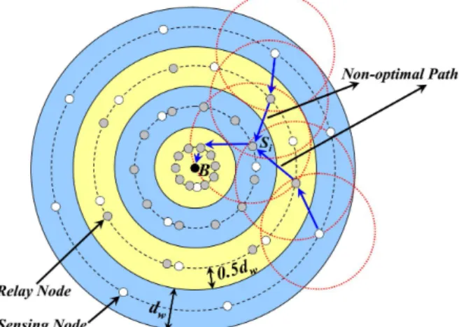
Fig. 14. Data uploading in SNAA [35]. 2
A. Values of the Coefficients of Virtual Force
3
It can be seen from Section III that, the value of λ and η will
4
determine the magnitude of the force to a large extent and
5
ultimately affect the distribution of nodes. Figure 15 shows
6
the results of node distribution with different values of λ and η
7
after the virtual force is applied. Without loss of generality, it
8
is assumed that 103 nodes are initially randomly deployed in
9
the circular network. To better show the nodes’ distribution in
10
different annuluses, boundaries of these annuluses (except the
11
network boundary) are painted with blue lines.
12
It is not difficult to know from figure 15(a) that, when
13
λ=0.4 and η=2000, the nodes’ distribution after virtual force
14
adjustment is not ideal. All nodes are clustered near the base
15
station and are located in the two innermost annuluses.
16
According to formula (3), we can see that the virtual force
17
between nodes in this case is mostly gravitation. The
18
magnitude of the repulsive force is close to or equal to the
19
virtual gravity only when the distance between nodes is very
20
short. Therefore, all nodes are close to the center of the
21
network due to the effect of gravitation. What’s more, when
22
the distance between each of them is short, the values of
23
virtual gravity and repulsion are equalized with each other so
24
that nodes will ultimately stay at or near the base station.
25
It can be seen from Figure 15(b) that the distribution of
26
nodes is relatively uniform in the case of λ=0.02 and η=12000,
27
but it tends to approach to the network boundary. This is
28
because most of the virtual force between nodes in this case
29
are repulsion. Only when the distance between them is short,
30
gravitation is generated (the repulsion is also large).
31
Therefore, nodes begin to stay away from the network center.
32
Since the boundary repulsive force is adopted in VFEM,
33
nodes can not move out of the network, but there are a
34
considerable number of nodes have moved to the vicinity of
35
the boundary.
36
From Section III.C-III.E, it is known that, neither of the
37
above cases can ensure the full coverage of the network. That
38
is, the virtual gravitation coefficient λ cannot be too small and
39
the virtual repulsion coefficient η cannot be too large.
40
By executing a mass of experiments, it is found that,
41
distribution of nodes after virtual force adjustment is ideal
42
when η=5400 and λ=0.23, as shown in Figure 15(c).
43 44 (a) η=2000, λ=0.4 (b) η=12000, λ=0.02 45 46 (c) η=5400, λ=0.23 47
Fig. 15. Distribution of nodes after virtual force adjustment. 48
B. Number of Nodes in Each Annulus
49
The mathematical expectations of the hop distance between
50
two nodes in adjacent annuluses are shown in Table II. Values
51
of these expectations are calculated by formula (15) when
52
R=100 and k takes 4, 5 and 6, respectively. It is not difficult to
53
find that when the value of k is unchanged, the hop distance
54
expectations of nodes are substantially equal to each other
55
except for the innermost annulus. So, for most of the relay
56
nodes, energy consumption on uploading one bit of data to their
57
next-hop successor are nearly the same. Although the closer to
58
the center of the network, the more the amount of data to be
59
uploaded by the relay nodes, the number of relay nodes located
60
in the vicinity of the network center is larger than that located in
61
other annuluses (as shown in Table III and Table IV). So, total
62
energy consumption of nodes in each annulus are basically the
63
same, which is consistent with the requirements of formula (7).
64
TABLE II 65
MATHEMATICAL EXPECTATIONS OF THE HOP DISTANCE 66
BETWEEN TWO NODES IN ADJACENT ANNULUSES 67 k=4 k=5 k=6 d0 12.5 m 10 m 8.3333 m d1 29.8094 m 23.8475 m 19.8729 m d2 29.5595 m 23.6476 m 19.7063 m d3 29.5309 m 23.6247 m 19.6873 m d4 - 23.6171 m 19.6810 m d5 - - 19.6781 m
Experimental results of the number of the sensing and relay
68
nodes in each annulus are shown in Table III and IV. It can be
69
found out that, total number of nodes is increasing from the
70
outermost annulus to the innermost one, but the increasing rate
71
has been slowing down. Total number of nodes in C1is very 72
close to that in C0. So, it can be concluded that VFEM can solve 73
the energy-hole problem by the optimal distribution of nodes
74
based on virtual force generated from annulus. In addition, the
75
number of sensing nodes in each annulus is small, which not
only ensures the full coverage of the whole network but also
1
minimizes the amount of the redundant data.
2
TABLE III 3
TOTAL NUMBER OF SENSING AND RELAY NODES IN EACH 4
ANNULUS (N=103, k=4) 5
Cm Nms Nmr Total number of Nodes
C0 1 35 36 C1 4 30 34 C2 7 17 24 C3 9 0 9 6 TABLE IV 7
TOTAL NUMBER OF SENSING AND RELAY NODES IN EACH 8
ANNULUS (N=200, k=5) 9
Cm Nms Nmr Total number of Nodes
C0 1 57 58
C1 4 52 56
C2 7 38 45
C3 9 21 30
C4 11 0 11
C. Residual Energy of Nodes in Each Annulus
10
Figure 16 and 17 show the residual energy of nodes in each
11
annulus at different network running times. Time of rounds at
12
the end of the network lifetime are 28956 and 34277,
13
respectively. The residual energy of each node in the
14
outermost annulus of the network at the same moment is
15
basically the same in any case. This is because in VFEM,
16
nodes in the outermost annulus are all sensing nodes and they
17
only need to upload their own sensed data to the next-hop
18
neighbor. As mentioned before, nodes in the outermost
19
annulus have the same amount of data to be uploaded in the
20
same period. Furthermore, it can be seen from Section III.E
21
that the lengths of single hop distances between nodes are
22
nearly the same with each other. So, lines in Figure 16(d) and
23
Figure 17(e) are substantially smooth.
24
Similarly, energy consumption of nodes in the innermost
25
annulus are also basically the same. This is because in VFEM,
26
most of nodes in the innermost annulus are relay nodes and the
27
hop distance for data uploading is only dw/2. Moreover, it is 28
known from Section III.D that, these relay nodes are uniformly
29
distributed in the center of the annulus, so it is almost no
30
difference among them on energy consumption.
31
Except for the innermost and the outermost annuluses, the
32
difference on energy consumption of nodes in other annuluses
33
is a little large. Residual energy of some nodes is too small.
34
According to the data collection path establishment method in
35
VFEM, it can be seen that not all nodes with forwarding
36
function are selected as the relay in the data upload path when
37
the network starts to run. Thus, the energy of some nodes can
38
be preserved at the beginning of the network lifetime, which
39
causes that the residual energy of nodes are different with
40
each other. However, it is not difficult to see from Figure
41
16(b), 16(c), 17(b), 17(c) and Figure 17(d) that at the end of
42
the network lifetime, the difference of the residual energy of
43
the nodes in these annuluses is not significant (e.g., the pink
44
lines in these figures). As the difference on energy
45
consumption between nodes continues to increase, some relay
46
nodes are unable to undertake the data uploading task, so the
47
sensing node are likely to reconstruct the routing path
48
according to formula (19). This realizes the energy balance
49
between nodes, and it effectively postpones the generation
50
time of energy-hole.
51
16 (a) 16 (b)
16 (c) 16 (d)
![Fig. 1. Network model of WSNEHA [30].](https://thumb-eu.123doks.com/thumbv2/5dokorg/4194650.91592/4.918.466.806.74.474/fig-network-model-of-wsneha.webp)


![Fig. 14. Data uploading in SNAA [35].](https://thumb-eu.123doks.com/thumbv2/5dokorg/4194650.91592/11.918.467.848.74.446/fig-data-uploading-in-snaa.webp)


