Mapping and assessment of ecosystems and their services

– the Swedish Forest Pilot

The Swedish Environmental Protection Agency Phone: + 46 (0)10-698 10 00, Fax: + 46 (0)10-698 10 99

E-mail: registrator@naturvardsverket.se

Address: Naturvårdsverket, SE-106 48 Stockholm, Sweden Internet: www.naturvardsverket.se

ISBN 978-91-620-6626-0 ISSN 0282-7298 © Naturvårdsverket 2014 Print: Arkitektkopia AB, Bromma 2014

Cover photos: Miljödepartementet

Förord

I denna rapport presenteras resultaten av ett pilotprojekt för kartläggning av ekosystemtjänster i skog inom projektet MAES1_{. Rapporten pekar på vilka}

tillgängliga dataflöden och indikatorer som kan användas för att göra en första bedömning av ekosystemens tillstånd och status avseende olika eko­ systemtjänster samt vilka dataflöden som behöver utökas eller kompletteras. En bedömning av ekosystemtjänster kan göras genom att befintliga data kom­ bineras och integreras med andra miljövariabler. Den svenska delen av studien undersökte därtill en metod för att kartlägga flera ekosystemtjänster i skog på nationell nivå baserat på prediktion med modeller som har passats till fältdata på ekosystemtjänster och befintliga miljövariabler.

Betydelsen av ekosystemtjänster har på senare tid blivit ett allt viktigare sätt för naturvården att visa hur tillståndet i ekosystemen och deras funktioner både direkt och indirekt bidrar till samhället. Mål om säkerställandet av eko system och deras tjänster återfinns både nationellt, på EU­nivå och inter­ nationellt. I Sverige har betydelsen av att säkra ekosystemens förmåga att långsiktigt generera ekosystemtjänster identifierats i både etappmål och i en av generationsmålets strecksatser. För att uppnå målen har det inom MAES projektet genomförts sex pilotstudier i syfte att syntetisera den information som finns på EU­ och medlemsstatnivå för att kartlägga, identifiera, prioritera och bedöma ekosystemtjänster.

MAES projektet visar att det finns en stor potential för att använda data som redan existerar men även att det finns återstående frågor att lösa i framtiden såsom mer forskning om sambanden mellan biologisk mångfald och eko­ systemtjänster. Det är också tydligt att ytterligare modellering och analyser av existerande data behövs innan en komplett kartläggning av ekosystemtjänster kan göras.

Rapporten är författad av Tord Snäll, Jon Moen, Håkan Berglund & Jan Bengtsson på Sveriges lantbruksuniversitet och Umeå universitet. Författarna svarar själva för rapportens innehåll. Den forskningsnära utred­ ningen har finansierats med medel från Naturvårdsverkets miljöforskningsanslag.

Stockholm september 2014

Contents

idEnTiFicATiOn OF dATA FOr EcOSySTEm mAPPing 10

Methods 10

rESulTS 12

Provisioning services 12

Regulating/maintenance services 13

Cultural services 16

Strengths and weaknesses 17

mAPPing mulTiPlE EcOSySTEm SErvicES 18

Aim 18

Materials and Methods 18

Data on ecosystem services from two nation-wide inventories 18

The three ecosystem services 19

Explanatory predictor variables 19

Statistical modelling 20

Results and Discussion 22

Detailed description of the final models for the ecosystem services 24

Identifying synergies, and trade-offs from ecosystem service maps 25

cOncluSiOnS 26

Sammanfattning

De övergripande målen för MAES projektet var att syntetisera den information som finns på EU­ och medlemsstatnivå när det gäller data och indikatorer som kan underlätta medlemsstaternas arbete för att i) identifiera och prioritera vilka ekosystemtjänster man vill kartlägga och bedöma; ii) identifiera vilka data som finns tillgängliga eller behövs; och iii) länka den biologiska mångfalden och ekosystemens tillstånd till ekosystemtjänster och mänskligt välbefinnande.

Det svenska pilotprojektet har bidragit till dessa mål för skogar, men pro­ jektet gick också ett steg längre genom att testa en metod för att kartlägga flera ekosystemtjänster i skog på en nationell nivå. Syftet med denna andra del av pilotstudien var att undersöka möjligheten att kartera ekosystemtjänster baserat på prediktion med modeller som har passats till fältdata på ekosystem­ tjänster och kartlagda miljövariabler som har erhållits genom modellering eller fjärranalys. Vi diskuterar också kort begränsningar när det gäller att identifiera synergier och avvägningar utifrån kartor över ekossystemtjänster.

MAES projektet visar att det finns en stor potential för att använda data som redan existerar och att kombinera dessa uppgifter i en enhetlig och inte­ grerad bedömning av ekosystemtjänster. De olika pilotprojekten har samlat en omfattande lista med indikatorer, som kan användas tillsammans med en typologi och karta av ekosystem, för att göra en första bedömning av eko­ systemens tillstånd och status på olika ekosystemtjänster. Men det finns också flera frågor som återstår att lösa i framtiden. Detta inbegriper mer forskning om sambanden mellan biologisk mångfald och ekosystemtjänster, särskilt för kulturella tjänster. Det är också tydligt att ytterligare modellering och analyser av existerande data behövs innan kartläggning kan göras.

När det gäller delprojektet om kartläggning, belyser detta projekt några av de möjligheter och svårigheter som finns att använda Riksskogstaxeringsdata för kartläggning av ekosystemtjänster på nationell nivå. Man måste bygga modeller för att kunna förutsäga nivån av ekosystemtjänster, där dessa mod­ eller begränsas av tillgången och upplösningen av potentiella förklarande variabler. Men vi bedömer också att kartor över ekosystemtjänster för olika livsmiljöer och för den biologiska mångfalden har potential att öka möjligheten för en ekosystembaserad förvaltning över olika sektorer, och därmed ligga till grund för en dialog mellan olika aktörer som har ett intresse för skog och eko­ systemtjänster i allmänhet. Detta kan vara särskilt viktigt i ett landskapspers­ pektiv, till exempel i samband med diskussioner kring en grön infrastruktur.

Summary

The overall objectives of the MAES (Mapping and Assessment of Ecosystem Services) project was to synthesise what information is available at EU and Member State scales in terms of data and indicators in order to facilitate Member States’ work when i)identifying and prioritising which ecosystems and services to map and assess; ii) identifying what data are available or needed; and iii) linking biodiversity and ecosystem condition to ecosystem services and human well­being.

The Swedish Forest pilot project contributed to these objectives for forests. However, it also went one step further to test an approach for mapping multi­ ple ecosystem services in forests at a national level. The aim of this second part of the pilot study was to investigate the potential to map ecosystem services based on prediction with models that have been fitted to field data on the eco­ system services as a function of mapped environmental variables that that have been obtained by modelling or remote sensing. We also briefly discuss limita­ tions to identify synergies and trade­offs from maps of ecosystem services.

The work undertaken by all the MAES Pilots in 2013 (including forests) shows that there is a big potential for using data that already exists and combining these data into a coherent and integrated ecosystem assessment. The pilots have assembled an extensive list of indicators, which can be used, together with a typology and map of ecosystems to make a first assessment of ecosystem condition and ecosystem services. However, there are also several issues that remain to be resolved in the future. This includes more research on the links between biodiversity and ecosystem services, in particular for cultural services. It is also clear that whereas data may already exist, for instance as NFI data, additional modelling and analyses are needed before mapping can be done.

As for the pilot mapping, this study highlights some of the possibilities, but also some of the difficulties in using NFI data for nation­wide mapping of ecosystem services. Models for the prediction of ecosystem services need to be built. These models are constrained by the availability and resolution of potential predictor variables that also have to be available on a national scale. However, ecosystem service maps for different habitats and for biodiversity provide opportunities to increase the potential for the management of ecosys­ tems and their services across sectors, and thus to form a basis for a dialogue for actors that have an interest in forest and ecosystem services in general. This could be especially important in landscape management, for instance in building a green infrastructure.

Background

Action 5 of the Biodiversity Strategy foresees that Member States will, with the assistance of the Commission, map and assess the state of ecosystems and their services in their national territory by 2014, assess the economic value of such services, and promote the integration of these values into accounting and reporting systems at EU and national level by 2020.

Based on this, the Working Group on Mapping and Assessment on Ecosystems and their Services (MAES) was mandated to coordinate and oversee Action 5. In 2012, the working group developed ideas for a coherent analytical framework to ensure consistent approaches are used. The report adopted in April 2013 proposed a conceptual framework linking biodiversity, ecosystem condition and ecosystem services to human well­being. Furthermore, it developed a typology for ecosystems in Europe and promoted the CICES classification for ecosystem services (ES henceforth).

Following the adoption of the analytical framework, the Working Group MAES decided to test it and in order to do so set up six thematic pilots. Four of the pilots focused on the main ecosystem types: agro­ecosystems (cropland and grassland), forest ecosystems, freshwater ecosystems (rivers, lakes, groundwater and wetlands), and marine ecosystems (transitional waters and marine inlets, coastal ecosystems, the shelf, the open ocean). Sweden, together with Portugal and the EU Joint Research Centre in Italy, took the lead of the forest pilot.

Forests cover around 40% of the EU land surface. The many interlinked roles of forest, from biodiversity conservation to timber provision, create multi­ sectoral and multi­objective characteristics of forest policies. There is a long history of EU measures supporting forest­related activities contributing to imple­ menting sustainable forest management, whereas coordination with Member States is developed mainly through the Standing Forestry Committee (SFC).

In September 2013, a new EU Forest Strategy for forest and the forest­based sector was presented with a new framework and wider scope in which forest protection, biodiversity conservation and the sustainable use and delivery of forest ecosystem services are addressed. Under the Strategy, sustainable forest management (SFM) is defined following MCPFE criteria: “SFM means using forests and forest land in a way, and at a rate, that maintains their biodiversity, productivity, regeneration capacity, vitality and their potential to fulfil, now and in the future, relevant ecological, economic and social functions, at local, national, and global levels, and that does not cause damage to other ecosystems”. SFM addresses current pressures on European forests from two different angles. Firstly, threats from environmental changes are expected to increase in the next years and decades, such as increasing water scarcity and pests, spread of invasive alien species, habitat loss, increased risk of forest fires, etc. Secondly, human­induced pressures such as forest fragmentation and over­exploitation of forest resources could impact negatively the provision, health and vitality of forest ecosystems. With this in mind the new Forest Strategy promotes

a coherent and holistic approach of forest management covering i) the multiple benefits and services of forests; ii) internal and external forest­policy issues and iii) the complete forest value­chain. From this perspective assessing, mapping and accounting of forest ecosystem services as foreseen under MAES, provides an integrated and systemic view of the forest system and the interlinked effects of the different pressures on forests. Ensuring forest protection and the delivery of forest ecosystem services is the overarching aim of the Strategy.

Objectives

The overall objectives of the MAES project was to synthesise what information is available at EU and Member State scales in terms of data and indicators in order to facilitate Member States’ work when:

• identifying and prioritising which ecosystems and services to map and assess;

• identifying what data are available or needed;

• making optimal use of EU environmental reporting streams;

• helping implement other actions of the EU 2020 Biodiversity Strategy; • guiding the use of information on ecosystem services in impact assess­

ments or in other policies;

• linking biodiversity and ecosystem condition to ecosystem services and human well­being.

The Swedish Forest pilot project contributed to these objectives for forests. However, it also went one step further to test an approach for mapping multi­ ple ecosystem services in forests at a national level. Specifically, the aim of this second part of the pilot study was to investigate the potential to map ecosystem services based on prediction with models that have been fitted to field data on the ecosystem services as a function of mapped environmental variables that that have been obtained by modelling or remote sensing. We also briefly dis­ cuss the limitations to identify synergies and trade­offs from maps of ecosystem services. We will describe both of these objectives in this report. A more com­ prehensive report on the identification of data for ecosystem mapping can be found in Maes et al. (2014).

Identification of data for

ecosystem mapping

All habitat pilots used a common typology for ecosystem mapping based on the key databases available at EU level. This typology should also allow for integration of assessments on national or sub­national levels based on more detailed classifications. The mapping of ecosystems is largely dependent on the availability of land­cover/land­use datasets at various spatial resolutions. The most comprehensive dataset for terrestrial and freshwater ecosystems at EU level is Corine Land Cover (CLC). However, the CLC data does not have the resolution needed for a more detailed ES mapping at the operational level, such as the one developed in this report. Also, ecosystem mapping should be based on the best available data from sub­national and national data sources at appropriate scales, to provide coherent information about ecosystems and their characteristics additional to EU level data.

Methods

The four thematic pilots followed a coordinated approach for information gathering, review and compiling of indicator lists. The approach was structured around four main steps.

Firstly, the Pilot leaders applied a table (referred to hereafter as the “MAES matrix”) including all ecosystem services using CICES v4.3 as baseline classi­ fication. An EU­wide MAES matrix of ecosystem services was populated from a literature review and assessing data and indicators available in the European data centres. After completion and agreement with the Pilot leaders, this matrix was sent to participating Commission services and stakeholders for review, addition of further data and agreement.

In a second step, participant MS and stakeholders from international and national organisations were requested to populate a country­level MAES matrix with relevant data and indicators available in their country. The resulting MAES matrices are available in CIRCABC (the European Commission Information Platform; https://circabc.europa.eu/).

The high level of detail and wide scope of the pilots yielded MAES matrices that required a supplementary level of synthesis for better access and readability. Thus, in a third step a series of “MAES cards” were implemented representing a synthesis of the information collected by the European and country­level MAES matrices. Each card focused on one service at a time and includes information on four aspects: reporting body, data availability of the indicator (six levels), units of measurement and compiling agency. The cards are more accessible and “readable” than the information included in the MAES matrices. The cards of the ecosystem pilots are included in a separate supplement to this report and could be used as a screening tool for deciding what indicators

are available for mapping and assessing biodiversity, ecosystem condition and ecosystem services. The cards were reviewed and agreed in a technical work­ shop held at the JRC in Ispra on 18 and 19 November 2013. The workshop brought together Member States, stakeholders and experts, members of the pilots, who contributed in several technical working sessions to the further refinement and agreement on the information included in the cards.

A fourth step of synthesis is included in the “MAES summary tables”, which are provided in this report as final outcomes of the pilots. The summary tables are built from the outcomes of the MAES cards and synthesized infor­ mation from the MAES matrices. The summary table is seen as the entry point for information regarding ecosystem services and potential indicators, proxies and datasets. It combines information provided by Member States and EU­level experts alike. The table is designed following the CICES classification and includes a colour key classifying indicators into four types:

Green: indicator for which harmonised, spatially­explicit data at the European scale is available and which is easily understood by policy makers or non­technical audiences.

Yellow: indicator for which either harmonised, spatially­explicit data at the European scale is unavailable, or which is used more than once in an ecosystem assessment which could possibly result in difficult interpretations by the user.

Red: indicator for which no harmonised, spatially­explicit data at the European scale is available and which only provides information at an aggregated level and which requires additional clarification to non­technical audiences.

Grey: indicators with unknown availability of reliable data and/or unknown ability to convey information to the policy making and implementation processes

The overview of data for forests (Maes et al. 2014), were produced by the Swedish team (Jan Bengtsson, Jon Moen and Tord Snäll) in cooperation with members of the MAES working group and research officers at JRC Ispra during several meetings between June 2013 and May 2014. In May 2014 Tord Snäll presented the Swedish work at High­level conference on mapping and assessment of ecosystems and their services in Europe, Brussels. The Forest pilot study was co­lead by Jose Barredo JRC, Ispra, Italy and Jan Bengtsson.

Results

In the following, we present the indicators for the forest services. The full tables for all habitats can be found in the MAES final report. The summary tables below are structured in three main sections of forest ecosystem services (FES) i.e. provisioning, regulating/maintenance and cultural services.

Provisioning services

The provisioning section (Table 1) includes the services related to forest produc­ tion of biomass, water and energy. In this section there are a reasonably large number of indicators in the green category. Most of these services are related to forest biomass supply and several available indicators are derived from data collected by National Forest Inventories (NFI) and from the European Forest Data Centre (EFDAC) for European level datasets. For these services, using data from NFI either as baseline for further assessment and/or mapping OR using it as data for model calibration/validation is the recommended option. Therefore, MS should use data from their NFI for mapping and assessment of Forest eco­ system services (FES) in this category. Other sources of information for forest biomass provision are remote sensing derived indicators that would in any case require ground information from NFI for model fitting and validation of results. Within the provisioning FES the situation regarding water­related services seems more problematic since no plug­ and­play indicators were identified and/ or addition of hydrological modelling techniques would be required for proper assessments. A few indicators were included for this category, most of them in the red category and only modelling­related indicators are green. Regarding provisioning services derived from plants and animals, most of the relevant indicators are in the yellow category, indicating a relatively good option for mapping and assessment, but requiring further work to be operational.

Table 1. indicators for provisioning services delivered by forests.

regulating/maintenance services

is because in this case the area of forest is a qualitative indicator from the per­ spective that it is able to indicate forested areas, but is unable to account for quantitative information about the supply of the service. Consequently the area of forest is considered to be a coarse indicator unable to convey relevant information to end­users and policy­makers. Therefore, further refined and/or local level assessments should be used for verifying the information provided by this type of indicator. This is applicable to other FES indicators coded in red in the summary table. Regarding the Division “Mediation of flows” green indicators are those derived from modelling exercises. In this case, more robust information can be provided. However, there is a need for the implementation of specific modelling approaches integrating different spatial datasets usually in a GIS environment or coupled with hydrological models, in particular for erosion protection, water supply and water flow maintenance. There is wide variability in the indicators identified in the Division “Maintenance of physical, chemical, biological conditions”. Four indicators are coded in green repre­ senting the most reliable sources of information for assessment and mapping. A closer look shows that for instance “abundance of pollinators” is an indica­ tor that should be streamlined with the agriculture pilot of MAES considering the strong links of these two ecosystems regarding pollinators. It is also notice­ able that for a number of indicators included in the red category more accurate local­level assessments could provide more reliable information to end­users and policy makers. One of the important services provided by forests regarding “global climate regulation” is carbon storage (and carbon sequestration). Indicators for this service could be computed from available proxy datasets derived from remote sensing imagery. See also the pilot mapping study below. Indicators for this service are coded in green and there is good availability of data at European and at country level.

cultural services

Forest cultural services include the non­material outputs of forest ecosystems. In this report cultural services should be regarded as the physical settings, locations or situations that produce benefits in the physical, intellectual or spiritual state of people. They can involve individual species, forest habitats and whole ecosystems. Forest cultural services are may be computed using multivariable analysis techniques in a GIS environment or using the modelling approach presented in this report. These techniques provide a cost­effective option for integration of a large number of explanatory variables into useful, spatially­explicit indicators. Further refined analyses computing the economic value of the recreational services provided by forests are feasible using value­ transfer and meta­analysis techniques. Some indicators included in the sum­ mary table (Table 3) are useful baseline data for further GIS­ or model­based analyses and/or recreational services quantification. Nevertheless, the indica­ tors on their own have a relatively low capacity for conveying relevant infor­ mation to end­users. This is shown in the summary table by the number of indicators identified in red. Another important aspect for cultural indicators is the availability and access of readily available data on, for instance, number of visitors, data on distribution of wildlife, number of hunters, etc. as well as the availability of GIS maps usually needed for computing spatial indicators such as accessibility to forested areas.

Strengths and weaknesses

Here we assess the strengths and weaknesses of the indicators included in the forest summary tables and propose some options for dealing with data gaps and the handling of red­coloured indicators.

The set of “green” indicators in the three tables are those for which information is readily available and that are able to convey valuable infor­ mation for end­users and policy­makers. These indicators are available at pan­ European and at country level and are considered reliable sources of information for the mapping and assessment of FES. Clearly, the indicators at pan­European level are usually coarser in spatial resolution (grid size of around 1 km) in comparison to country­level indicators where finer spatial resolution and higher accuracy of the measured variable is expected e.g. forest biomass provision. This is also necessary for the planning at the local, opera­ tional level.

NFI data should play an important role in the assessment and mapping of FES, as exemplified below in this report. NFIs are the main sources of forest information at country level and of the harmonized data collections held by EFDAC (FISE). Therefore, their use is the suggested option for first hand data and indicators of forests services. In some cases further refinement and analysis should be implemented using NFI data for building indicators of FES, other­ wise they can be used as baseline data for calibrating and validating models used for implementing FES indicators.

Among the main limitations of the indicators in the summary table it is necessary to consider the opportunity for the proper use of “red” indicators. In many cases they are qualitative indicators (e.g. forest/non forest maps) and are not adequate for allowing an estimation of the supply of services, which should be based on quantitative information. The alternative of using quali­ tative indicators for measuring supply or stock of a given service is a limited option for providing information to the policy­makers. Quantitative validated indicators are the suggested option for this purpose. This is an aspect that should be carefully considered in the methodological step of the implementa­ tion of mapping and assessment of FES.

In the following we present an approach for mapping FES that have been measured by the Swedish National Forest Inventory. It allows mapping the FES at the operational scale at which local decision making takes place.

Mapping multiple ecosystem services

Aim

The aim of this part of the pilot study is to investigate whether there are sig­ nificant relationships between field measurements on ecosystem services and mapped environmental variables that that have been obtained by modelling or remote sensing. If significant relationships to the mapped variables are found, then regression modelling and prediction should be a superior approach for ecosystem service mapping compared to spatial interpolation of the field measurements on the services. Finally, we briefly discuss the limitations to identify synergies, and trade­offs from maps of ecosystem services.

Materials and Methods

data on ecosystem services from two nation-wide inventories

We used a nation­wide forest data set from the National Forest Inventory and the Survey of Forest Soils and Vegetation, covering an area of 400,000 km2

of production forests. Hereafter the inventories are referred to as the NFI. The inventory uses a randomly planned regular sampling grid covering the whole country (Axelsson et al. 2010), and includes around 4,500 permanent tracts with each tract being surveyed once every 5 years. The tracts, which are rectangular in shape and are of different dimensions in different parts of the country, consists of 8 (in the north) to 4 (in the south) circular sample plots (each plot 314 m2_{). Tree biomass and production are measured in all plots}

whereas soil data and the cover of bilberry are recorded in about half of the plots. We only used plots from which we had data on the respective response variable and all explanatory variables, leading to different sample sizes for the ecosystem services (Table 4). From the NFI database we extracted data from 1999 to 2002, which represents one complete survey. We used only plots on “productive forest” (average production of standing volume, stem volume over bark >1 m3 _ha–1 _year–1_{), which had not been harvested, cleared,}

or thinned during the previous five years before the survey. The previous time period of five years was also used for calculating biomass production. To be included in our analyses, the plots had to be located on only forest land, i.e. not including any river, road, grassland, etc. We excluded plots where the bio­ mass production of any of the focal tree species was greater than the 99% per­ centile (which is standard procedure in analyses of data from the NFI). This procedure excluded plots with unrealistically high values of production.

The three ecosystem services

Tree biomass production was estimated as the yearly change in tree biomass

(kg m–2 _year–1_{), calculated over a period of 5 years, and for all tree individuals}

higher than 1.3 m. For plots visited in the years 1999–2002, the baseline for biomass production was thus the years 1994–1997. Biomass was calculated with biomass functions (Marklund 1988, Petersson and Ståhl 2006) and was the sum of the biomass from the stem, twigs and branches, the stump and roots. For deciduous tree species, there is only a function for Betula spp., and this function was applied for all other deciduous tree species. The function for Pinus sylvestris was applied for Larix decidua and Pinus contorta. Even though this creates a slight tree species bias, it has minor effects on our pro­ duction estimates since we compared the biomass of the trees at two points in time. The sample size was 3,900 plots distributed across 798 tracts (Table 1).

Soil carbon storage was measured as the amount of carbon (g m–2_{) in the}

topsoil, which consisted of either purely organic horizons, i.e. mor layers (63%) or peat layers (21%), or less frequently of minerogenic A­horizons (16%). This is the part of the soil most affected by the current above­ground biota. To compensate for the conceptual difference in topsoil types, mean soil carbon stocks were set equal for purely organic soils (measured in the organic horizon down to a maximum depth of 30 cm) and minerogenic topsoils (measured in the top 10 cm horizon). The soil fraction <2 mm was analyzed. Soil sampling was carried out on around 50% of the inventory plots (Table 1). Data were log­transformed.

Bilberry production was measured as the percentage of each plot covered

by bilberry, Vaccinium myrtillus. The cover of V. myrtillus is strongly corre­ lated to annual production. Bilberry is one of the economically most important wild berry species in Northern Europe (Miina et al. 2008). Bilberry sampling was carried out on around 50% of the inventory plots (Table 4). Data were converted to proportions and arcsine transformed, after correcting for the area where berries could not grow, e.g. the area of stems and boulders.

Explanatory predictor variables

Since the overall aim of the modelling was to map the ecosystem services by making model predictions, we used only explanatory variables for which we had nation­wide mapped data. The set of variables chosen was based on Gamfeldt et al. (2013). There we used a more extensive set that had been measured on the plots, but since not all variables in Gamfeldt et al. (2013) have been mapped throughout the landscape, we could not use all of them in the current modelling and model prediction mapping.

sent models was set to four, specifically when the volume was >0 of each of spruce, pine, birch and other broad­leaved tree species. Finally, we used altitude and a soil moisture index as explanatory variables.

The climate variables were calculated based on the gridded dataset

“PTHBV” produced by the Swedish Meteorological and Hydrological Institute (SMHI). The dataset includes daily precipitation and daily mean temperature from 1961–2010 and has a resolution of 4 km all over Sweden. The cell values are estimated based on meteorological observations using an optimum interpolation procedure (Johansson 2000; Johansson and Chen 2003; 2005). The values of the forest stand variables were based on estimates combining satellite images and field data from the NFI from 2000, and has a resolution of 25 m, ‘kNN­Sweden 2000’ (http://skogskarta.slu.se/, Reese et al. 2002). The altitude was obtained from a digital topographic map with a cell size of 50 m (Geografiska Sverigedata 2010). The soil moisture index was calculated according to Stein (1994) using the digital topographic map.

Statistical modelling

We modelled the three ecosystem services by linear mixed­effects modelling (Bates et al. 2013). The effect of the climate variables were modelled at the tract scale (random effects), while the effect of the remaining variables were modelled at the plot scale (fixed effects).

Prior to the modelling we transformed bilberry cover and soil carbon stor­ age (see above). We also centred and standardized the explanatory variables (subtracted the mean and divided by standard deviation, Table 5). Thus, the size of the parameter estimate for each explanatory variable (Table 4) can con­ sidered an estimate of the relative importance of the variable (effect­size). Note, however, that when a variable is squared or is included in an interaction term, the interpretation of the relative importance of the variable, as well as whether the relationship with the variable is positive or negative may be difficult.

Table 4. Explanatory predictor variables, standardized estimates of parameters (standard errors) and diagnostics for mixed-effect regression models for three ecosystem services on productive forest land. Predictor variable Wood production Bilberry cover Soil carbon storage

Intercept 0.575 (0.007) 18.7 (0.393) 7.87 (0.020)

Length of vegetation period (LVP) a _{–0.028 (0.007) –3.13 (0.439) 0.10 (0.031)}

Summed precipitation April–October (Precip.) 0.877 (0.343) 0.11 (0.025)

Stand age (years) –0.167 (0.009) 2.013 (0.388)

Spruce b _{0.254 (0.010) –0.662 (0.357)}

Pine b _{0.066 (0.008) 2.94 (0.377)}

Birch b _{0.037 (0.006) 0.577 (0.284) 0.07 (0.019)}

Other broad-leaved trees b _{0.020 (0.006) –1.144 (0.278)}

Species richness c _{0.028 (0.006) 0.684 (0.294)}

Altitude (m) 1.288 (0.379) –0.10 (0.027)

Soil moisture –1.623 (0.303) 0.16 (0.019)

Soil moisture2 _{0.380 (0.169)}

Spruce x Stand age –0.179 (0.008) 0.873 (0.310)

Pine x Stand age –0.060 (0.006) –1.427 (0.301)

Birch x Stand age –0.033 (0.008)

LVP x Spruce –0.075 (0.007)

LVP x Birch –0.017 (0.005) –0.617 (0.251)

Precip. x Spruce –0.488 (0.249)

Tract standard deviation 0.05 4.11 0.20

Residual standard deviation 0.31 9.71 0.76

Deviance 2,095.1 14,390.3 4,080.0

AIC d _{2,234 14,439 4,131}

Number of plots 3,900 1,915 1,742

Number of tracts 798 698 679

Plot-level (marginal) R2 e _{0.35 0.27 0.13}

Full model (conditional) R2 e _{0.37 0.38 0.18}

a _{Number of days between the fourth day in the first four-day period with a 24 hours mean temperature}

of +5° C and the last day with this mean temperature.

b _m3_/ha.

c _{Maximum four, when the volume of spruce, pine, birch and other deciduous trees are all >0.} d _{Akaike’s Information Criterion.}

e _{according to Nakagawa and Schielzeth (2013).}

Table 5. mean and standard deviation of the explanatory predictor variables included in the final models for three ecosystem services (Table 4).

Predictor variable mean Standard deviation

Length of vegetation period a _{214.5 44.0}

Summed precipitation April–October 473.9 93.1

Stand age (years) 58.5 35.1

Spruce b _{62.8 78.1}

Pine b _{53.5 51.4}

We built the final models based on Akaike’s Information Criterion (AIC; Akaike 1974), on the estimates of the effect­size parameters, on knowledge of the biological system studied, and on Gamfeldt et al. (2013). We first assessed the predictive power of each explanatory variable based on AIC and on the effect­size parameters. Next, we fitted a multiple model containing the retained explanatory variables, biologically reasonable squared terms and interactions. Finally, we simplified this multiple model by excluding and again including earlier excluded variables in a stepwise procedure.

We quantified the predictive ability of each model by R2_{, i.e. the variance}

explained by the model. The estimator R2 _{for mixed­effect models according to}

Nakagawa and Schielzeth (2013) was applied. It allows separating plot­level (marginal, fixed effects) R2 _{from full model (conditional, i.e. including also}

the tract level (random) effects) R2_{. The models were fitted using the statistics}

software R 3.0.1 (R Development Core Team 2013) and library lmer4 (Bates et al. 2013).

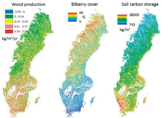
Figure 1. Mapped ecosystem services based on regression modelling of field measurements on eco-system services on productive forest land and mapped environmental variables that that have been obtained by modelling or remote sensing. The regression models used are presented in Table 4.

Results and Discussion

Our final models are similar to the models that resulted from using NFI field measurements on also the explanatory variables (Gamfeldt et al. 2013). More specifically, for each ecosystem service the explanatory variables included in the final model were similar to the variables in Gamfeldt et al. (2013).

Also the qualitative relationships (positive/negative), the non­linearities, and the interactions between the explanatory variables were similar to Gamfeldt et al. (2013). However, in the current study fewer relationships were signifi­ cant. The probable explanation is the less accurate data on the explanatory variables, which in the present case had been obtained by modelling or remote sensing.

The national­scale mapping of the ecosystem services are biologically rea­ sonable (Fig. 1), as detailed below. The mapping is also similar to preceding national mappings of these services (Lind 2001, Skogsdata 2011, Sveriges Nationalatlas 2011). These preceding mappings are based on interpolating the NFI plot­level measurements on the ecosystem services. That is, in the mapping they do not utilize information on the environmental conditions between the NFI plots that affect the ecosystem service levels. In the current study we utilize such information, specifically the mapped explanatory varia­ bles. This means that the current study should provide more accurate mapping of the ecosystem services than the preceding mappings.

Although our regression modelling and prediction approach is advocated for ecosystem service mapping (Martinez­Harms and Balvanera 2012), the predicted magnitude of the ecosystem services at the smallest spatial scale, 25 m × 25 m, is imprecise. Specifically, the variance explained by the models (R2_{) is not high – 35–40% for wood production and bilberry cover and 18%}

for soil carbon storage (Table 4). However, as described above the models are similar to models that have utilized field measurements on the explanatory variables (Gamfeldt et al. 2013). Moreover, as developed in the detailed description below, the models are biologically reasonable.

There are many ways to improve the predictive ability of these models, or in other words, to increase the variance explained by the models. First, addi­ tional explanatory variables can be included in the model building. The models in Gamfeldt et al. (2013) include about twice the number of explanatory vari­ ables that we utilized. Additional and more mechanistically important climate variables can be added. Also variables on soil conditions can be added. For example, Gamfeldt et al. (2013) found difference in soil carbon storage between plots on peat and on non­peat soils, and if we add this variable to the current model, the variance explained (R2_{) increases from 18 to 32% (not shown). Also,}

more accurate data on the explanatory variables can be used. For example, the Swedish Meteorological and Hydrological Institute is currently producing maps on climate variables with higher spatial resolution and accuracy than the maps that we have used. The algorithm used for the soil moisture index can be improved. The mapped kNN forest variables that we have used are known to have low accuracy at the level of pixels (Reese et al. 2003), and it may be better

data from 2000 to today, representing the whole period for which kNN­data on the forest variables are available (every fifth year since 2000). However, given the limited budget for the modelling in the current pilot study, using these additional or alternative data was not possible.

detailed description of the final models for the ecosystem services

There was a clear latitudinal gradient in wood production with high levels in the south (Fig. 1). Nevertheless, the relationships between wood production and length of the vegetation period are negative (Table 4). The likely explanation is that the variable is included in interactions with the volume of the different tree species. As mentioned in Statistical modelling above, the interpretation of the relationship with a variable that is also included in a interaction term may be difficult. Wood production increased with increasing tree volumes (the estimates are positive) but the strengths of these relationships decreased with increasing length of the vegetation period (the interaction is negative). Moreover, the positive relationship with the volumes decreased with increasing stand age. The relationship between wood production and the main effect stand age was also negative. Finally, production increased with increasing tree species richness. Potential mechanisms behind positive relationships between production and species richness are discussed in Gamfeldt et al. (2013).

There was a clear latitudinal gradient also in bilberry cover with lowest cover in the south (Fig. 1), where the field layer is more commonly dominated by herbs and grasses rather than by Ericaceae species such as bilberry (Skogsdata 2011). More specifically, bilberry cover generally increased with increasing altitude and precipitation, and decreased with the length of the vegetation period (Table 4). The positive relationship with precipitation was reduced as the spruce volume increased (the interaction is negative). The likely explana­ tion is that the field layer in the southern regions with high spruce volume and precipitation is usually dominated by herbs or grasses. The negative relation­ ship to length of the vegetation with increasing birch volume (the interaction is negative) probably reflects that the field­layer also in the birch forests in the south is dominated by herbs or grasses. Bilberry cover also increased with increasing stand age. The increase with age was particularly high when also the spruce volume increased (positive interaction), probably reflecting the gen­ eral pattern that bilberry shows low cover in young spruce forest. In contrast, bilberry cover decreased with increasingly older pine forest (negative interac­ tion). Finally, there was a negative, non­linear relationship with soil moisture.

Also the soil carbon storage showed a clear latitudinal gradient with high­ est levels in the south (Fig. 1). The soil carbon storage increased with increas­ ing length of the vegetation period and precipitation, while it decreased with altitude (Table 4). At the local scale it increased with increasing birch biomass and particularly with soil moisture. The strong positive effect of increasing soil moisture (large effect­size, Table 4) probably partly reflects the substan­ tially higher carbon storage on peat (high soil moisture) than on non­peat plots (lower soil moisture) (see above and Gamfeldt et al. 2013).

identifying synergies, and trade-offs from ecosystem service maps

Maps of ecosystem services can be used to identify sites with high or low levels of focal services (hotspots and coldspots, respectively), sites with high levels of a specific service or sites with intermediate levels of the services. However, the maps have limitations concerning identifying synergies, trade­offs or conflicts. A hotspot site may indicate a synergy if the extraction of one service does not decrease the level of the other service, i.e. if they are independent. In con­ trast, it may indicate a possible conflict if the management for one service (including extraction) decreases the level of the other one. The underlying mechanisms may be direct in the form of changed interactions between the services, or indirect resulting from changed environmental conditions. Here, a dialogue on trade­offs between the groups representing the services is neces­ sary for appropriate management.

Also the mechanisms explaining a site with low (coldspot) or intermediate levels of the ecosystem services are difficult to identify. At a coldspot the natural environmental conditions may be poor for both services. These natural envi­ ronmental conditions may or may not be possible to change with management. Another mechanism explaining a coldspot site of focal services may be inter­ actions with another unmeasured service or driver. This interaction may be natural or result from management for the unknown service. It is also possible, but less likely, that low levels of both services result from negative interactions between them.

High levels of one service but not of another on a particular site may also be explained by natural environmental conditions, negative interactions or management benefitting only one of the services. However, at these sites we observe the result of these processes or conditions having had their effect, and further analyses are necessary to elucidate the reasons behind the observations.

Conclusions

The work undertaken by all the MAES Pilots in 2013 shows that there is a big potential for using data that already exists and combining these data into a coherent and integrated ecosystem assessment. The pilots have assembled an extensive list of indicators, which can be used, together with a typology and map of ecosystems to make a first assessment of ecosystem condition and ecosystem services. However, there are also several issues that remain to be resolved in the future. This includes more research on the links between biodi­ versity and ecosystem services, in particular for cultural services, the relations between forests and water services, and how to understand and manage syner­ gies, trade­offs among services. It is also clear that whereas data may already exist, for instance as NFI data, additional modelling and analyses are needed before mapping can be done.

As for the pilot mapping, this study highlights some of the possibilities, but also some of the difficulties in using NFI data for nation­wide mapping of ecosystem services. Models for the prediction of ecosystem services need to be built. These models are constrained by the availability and resolution of potential predictor variables that also have to be available in mapped format. There are also limitations concerning identifying sites of synergy or trade­off. Nevertheless, ES maps for different habitats and for biodiversity have the potential to increase the potential for the management of ecosystems and their services across sectors, and thus to form a basis for a dialogue for actors that have an interest in forest and ecosystem services in general. This could be especially important in landscape management, for instance in building a green infrastructure (Snäll et al. in review).

References

Akaike, H. 1974. A new look at statistical model identification. IEEE Transactions on Automatic Control AC, 19, 716–722.

Axelsson, A.­L., Ståhl, G., Söderberg, U., Petersson, H., Fridman, J., and Lundström, A. 2010. In National Forest Inventories—Pathways for Common Reporting. (eds Tomppo, E., Gschwantner, Th., Lawrence, M. & McRoberts, R. E.) 541–553, Springer.

Bates, D., Maechler, M., and Bolker, B. 2013. lme4: Linear Mixed­Effects Models Using S4 Classes. R package version 1.1­6,

URL http://CRAN.R­project.org/package=lme4.

Gamfeldt, L., Snäll, T., Bagchi, R., Jonsson, M., Gustafsson, L., Kjellander, P., Ruiz­Jaen, M.C., Fröberg, M., Stendahl, J., Philipson, C.D., Mikusiński, G., Andersson, E., Westerlund, B., Andrén, H., Moberg, F., Moen, J. and Bengtsson, J. More diverse forests support higher levels of ecosystem services and functions. Nature Communications, 4, 1340.

Geografiska Sverigedata. 2010. GSD­Höjddata, grid 50+. Lantmäteriet. Johansson, B. 2000. Areal Precipitation and Temperature in the Swedish Mountains. An evaluation from a hydrological perspective. Nordic Hydrology, 31, 207–228.

Johansson, B. and Chen, D. 2003. The influence of wind and topography on precipitation distribution in Sweden: Statistical analysis and modelling. International Journal of Climatology, 23, 1523–1535.

Johansson, B. and Chen, D. 2005. Estimation of areal precipitation for runoff modelling using wind data: a case study in Sweden. Climate Research, 29, 53–61.

Lind, T. 2001. Kolinnehåll i skog och mark i Sverige – Baserat på

Riksskogstaxeringens data. Arbetsrapport 86. Institutionen för skoglig resurs­ hushållning och geomatik, Sveriges lantbruksuniversitet. ISSN 1401–1204. Maes, J., Teller, A., Erhard, M., Murphy, P., Paracchini, M.L., Barredo, J.I., Grizzetti, B., Cardoso, A., Somma, F., Petersen, J.­E., Meiner, A., Gelabert, E.R., Zal, N., Kristensen, P., Bastrup­Birk, A., Biala, K., Romao, C., Piroddi, C., Egoh, B., Fiorina, C., Santos, F., Naruševičius, V., Verboven, J., Pereira, H., Bengtsson, J., Kremena, G., Marta­Pedroso, C., Snäll, T., Estreguil, C., San Miguel, J., Braat, L., Grêt­Regamey, A., Perez­Soba, M., Degeorges, P.,

Marklund, L.G. 1988. Biomass Functions for Pine, Spruce and Birch in Sweden (Department of Forest Survey, SLU).

Martinez­Harms, M.J. and Balvanera, P. 2012. Methods for mapping eco­ system service supply: a review. International Journal of Biodiversity Science Ecosystem Services Management, 8, 17–25.

Miina, J., Hotanen, J. P. and Salo, K. 2009. Modelling the abundance and temporal variation in the production of bilberry (Vaccinium myrtillus L.) in Finnish mineral soil forests. Silva Fennica, 43, 577–593.

Nakagawa, S. and Schielzeth, H. 2013. A general and simple method for obtaining R2 _{from generalized linear mixed­effects models. Methods in}

Ecology and Evolution, 4, 133–142.

Petersson, H. and Ståhl, G. 2006. Functions for Below­Ground Biomass of Pinus Sylvestris, Picea Abies, Betula Pendula and Betula Pubescens in Sweden (Department of Forest Resource Management and Geomatics, SLU).

R Development Core Team. 2013. R: A language and environment for statistical computing. R Foundation for Statistical Computing, Vienna.

Reese, H., Nilsson, M., Granqvist Pahlén, T., Hagner, O., Joyce, S., Tingelöf, U., Egberth, M. and Olsson, H. 2003. Countrywide Estimates of Forest Variables Using Satellite Data and Field Data from the National Forest Inventory. Ambio, 32, 542–548.

Reese, H., Nilsson, M., Sandström, P. and Olsson, H. 2002. Applications using estimates of forest parameters derived from satellite and forest inventory data Computers and Electronics in Agriculture, 37, 37–55.

Skogsdata. 2011. Aktuella uppgifter om de svenska skogarna från

Riksskogstaxeringen Tema: Fält­ och bottenskiktsvegetation i Sveriges skogar. Institutionen för skoglig resurshushållning, SLU.

Skogsstatistik. 2014. http://www.slu.se/sv/centrumbildningar­och­projekt/ riksskogstaxeringen/tjanster­och­produkter/interaktiva­tjanster/slu­skogskarta/ Snäll,T., Lehtomäki, J., Arponen, A., Elith, J. and Moilanen, A. In review. Green infrastructure design based on spatial conservation prioritization and modeling of citizen science data and ecosystem services.

Stein, J.L. 1994. Unpublished Arc/Info aml based on original Fortran code by M.F. Hutchinson, B.G. Mackey and J.A. Stein, Fenner School of Environment and Society, Australian National University, Canberra, ACT.

Sveriges Nationalatlas. 2011. Jordbruk och skogsbruk i Sverige sedan år 1900: studier av de areella näringarnas geografi och historia. SNA.

The authors assume sole responsibility for the con-tents of this report, which

therefore cannot be cited as representing the views of the Swedish EPA.

KUNSKAP DRIVER MILJÖARBETET FRAMÅT

ISSN 0282-7298

TORD SNÄLL, JON MOEN,

HÅKAN BERGLUND & JAN BENGTSSON

This report provides an introduction to possible approaches for mapping and assessment of forest ecosystem services based on spatial information and indicators. Criteria for mapping Europe’s ecosystems and their services are explored through several pilot studies within the project MAES. An approach for mapping and identifying synergies and trade-offs of multiple ecosystem services was tested, aiming to investigate the potential to map ecosystem services based on prediction with models. Mapping and assessment of ecosystem services will generally be possible by combining currently available ecosystem data with environment variables, however some constrains still remain. Ecosystem services provides a framework that links human societies and their well-being with the environment, and knowledge relating to ecosystems their functioning, status and trends, and the consequences of their loss must constantly be improved. The MAES working group is part of the implementation of the EU Biodiversity Strategy to 2020. The aim is to support and contribute to a consistent mapping and assessment of ecosystems within the EU. The study was financed by the Swedish Environmental Protection Agency.

their services

The Swedish Forest Pilot

HÅKAN BERGLUND & JAN BENGTSSON

Mapping and assessment

of ecosystems and

their services

The Swedish Forest Pilot

rEPOrt 6626 • OCTOBER 2014 3. 4. 5. 6. 12. 15. 14. 11. 4. 5 15 3. 4 6. 12. 14. 111.1..