Passive control of mechanical systems

Full text

(1)TRITA-MEK ISSN 0348-467X ISRN KTH/MEK/TR--01/06--SE. Passive Control of Mechanical Systems Bipedal Walking and Autobalancing by Jesper Adolfsson. May 2001 Technical Reports from Royal Institute of Technology Department of Mechanics S-100 44 Stockholm, Sweden.

(2) Akademisk avhandling som med tillstånd av Kungliga Tekniska Högskolan i Stockholm framlägges till offentlig granskning för avläggande av teknologie doktorsexamen fredagen den 11:e maj 2001 kl 11.00 i hörsal M3, Brinellvägen 64, Kungliga Tekniska Högskolan, Stockholm. ãJesper Adolfsson 2001.

(3) Passive Control of Mechanical Systems: Bipedal Walking and Autobalancing Jesper Adolfsson 2001. Department of Mechanics, Royal Institute of Technology S-100 44 Stockholm, Sweden. Abstract. This thesis explores the dynamics of two mechanical systems capable of performing their tasks without the use of active control. The first system is an autobalancer, which can continuously balance rotating machinery. This is accomplished by using compensating masses that move in a viscous media about the axis of rotation. The second system is a passive bipedal walker, capable of human like gait in the absence of external active control. Since there is no control system to suppress errors in the mechanisms it is important to have a detailed knowledge of how parameters influence on these systems. The dynamics of mechanical models, such as the three dimensional passive walker and autobalancer, are explored and understood using standard dynamical systems methods. This includes calculating the stability of equilibrium positions and limit cycles and creating bifurcation diagrams as parameters of the system are varied. In the case of the autobalancer it is possible to analytically solve for the equilibrium positions. In the passive walker the stability of limit cycles, which corresponds to periodic gaits, are studied. To find these limit cycles a Newton-Raphson root solving scheme is implemented. The model for the autobalancer results in a smooth dynamical system whereas the passive walker includes different kinds of discontinuities. These discontinuities are taken care of by introducing suitable mappings. Results for the autobalancer include suggestions on how to choose parameters of the systems and how to avoid possible dangerous parameter combinations. It also explains some experimentally observed limit cycles. In the case of the passive walker, it is shown how the planar passive walker extended into a fully three dimensional walker having dynamics in all directions. Many parameter studies are reported which give an insight dynamics of the system. The thesis ends with an report on the search implementable passive walker.. can be spatial to the for an. The methods introduced in this thesis are not limited to the study of autobalancing and passive bipedal walking but are applicable to many mechanical systems with or without discontinuities. Descriptors: autobalancing, bipedal walking, multibody systems, nonlinear dynamics, stability, bifurcations, limit cycles, variational equations, discontinuities.

(4)

(5) Preface This thesis present studies, made on two di¤erent passive mechanical systems, the Autobalancer, capable of passively balancing rotating unbalance and the passive walker, capable of human like bipedal gait without using active control. This thesis includes modeling assumptions, simulations, and analysis performed on these systems. It is based on the following papers; Paper 1 Adolfsson, J.: 1997 ‘A Study of Stability in Autobalancing Systems using Multiple Correction Masses’, Technical Report, KTH, Department of Mechanics Paper 2 Adolfsson, J.: 2000 ‘A short introduction to walking’, Technical Report, KTH, Department of Mechanics Paper 3 Adolfsson, J. & Nordmark, A.: 2000 ‘Planar Passive Walkers: Code Implementation Issues’, Technical Report, KTH, Department of Mechanics Paper 4 Adolfsson, J., Dankowicz H., & Nordmark, A.: 1998 ‘3-D Stable Gait in Passive Bipedal Mechanisms’, In Proceedings of Euromech 375, Biology and Technology of Walking, pp 253-259 Paper 5 Adolfsson, J., Dankowicz H., & Nordmark, A.: 2000 ‘3D Passive Walkers: Finding Periodic Gaits in the Presence of Discontinuities’, In Nonlinear Dynamics, Volume 24, Number 2, February 2001, pp. 205-229 Paper 6 Dankowicz H., Adolfsson, J., & Nordmark, A.: 1998 ‘Existence of Stable 3D-Gait in Passive Bipedal Mechanisms’, In Journal of Biomechanical Engineering, Volume 123, Number 1, February 2001, pp. 40-46 Paper 7 Adolfsson, J.: 2000 ‘3D Passive walkers: Code Implementation Issues’, Technical Report, KTH, Department of Mechanics Paper 8 Adolfsson, J.: 2000 ‘Finding an Implementable 3D Passive Walker using Continuation Methods’, Technical Report, KTH, Department of Mechanics The papers are here re-set in the present used thesis format. Some of them are published as indicated above..

(6)

(7) Contents 1 Introduction. 1. 2 AutoBalancing 2.1 Background . . . . . . . . . . . . . . . . . . . . . . . . . . . . . . 2.2 AutoBalancer . . . . . . . . . . . . . . . . . . . . . . . . . . . . . 2.3 Conclusion . . . . . . . . . . . . . . . . . . . . . . . . . . . . . .. 3 3 4 7. 3 3D 3.1 3.2 3.3 3.4 3.5. Passive Walking Background . . . . . . . . . . 3D passive walker . . . . . . . Numerical simulation . . . . . Finding an implementable 3D Conclusion . . . . . . . . . .. . . . . . . . . . . . . . . . . . . . . . . . . . . . passive walker . . . . . . . . .. . . . . .. . . . . .. . . . . .. . . . . .. . . . . .. . . . . .. . . . . .. . . . . .. . . . . .. . . . . .. . . . . .. 9 9 11 12 13 14. 4 Mechanics 15 4.1 Sophia . . . . . . . . . . . . . . . . . . . . . . . . . . . . . . . . . 18 5 Analysis methods 5.1 Nonlinear dynamics . . . . . . . . . . . 5.1.1 Flow . . . . . . . . . . . . . . . . 5.1.2 Limit cycles . . . . . . . . . . . . 5.1.3 Stability of the dynamical system 5.1.4 Stability of limit cycles . . . . . 5.1.5 Finding limit cycles . . . . . . . 5.1.6 Variational equations . . . . . . . 5.1.7 Discontinuities . . . . . . . . . . 5.2 Bifurcations . . . . . . . . . . . . . . . . 5.2.1 Saddle-node bifurcations . . . . . 5.2.2 Pitchfork bifurcations . . . . . . 5.2.3 Hopf bifurcations . . . . . . . . . 5.2.4 Period doubling . . . . . . . . . . 5.3 Conclusion . . . . . . . . . . . . . . . . 6 Acknowledgements. . . . . . . . . . . . . . .. . . . . . . . . . . . . . .. . . . . . . . . . . . . . .. . . . . . . . . . . . . . .. . . . . . . . . . . . . . .. . . . . . . . . . . . . . .. . . . . . . . . . . . . . .. . . . . . . . . . . . . . .. . . . . . . . . . . . . . .. . . . . . . . . . . . . . .. . . . . . . . . . . . . . .. . . . . . . . . . . . . . .. . . . . . . . . . . . . . .. . . . . . . . . . . . . . .. 21 21 21 22 22 23 24 25 25 26 27 27 27 28 28 31.

(8)

(9) Chapter 1. Introduction In our everyday life, we are surrounded by mechanisms, which perform many di¤erent tasks. The operation of most of these mechanisms can be understood intuitively by just looking at them. Examples of such mechanisms are wheels, pulleys, chains, link mechanisms, and even devices such as automotive vehicles. At the time of their invention, most of them have been made to work by cleverness and ingenuity, without a need for deeper theoretical understanding. As the theory of Newtonian mechanics was developed by Newton in 1666, it became possible to re…ne and optimize their operation by making theoretical models of the mechanisms. These theoretical models could now answer questions about the mechanism without constantly having to build new prototype mechanisms. Thus, greatly enhancing the understanding of the mechanism and thereby increasing the speed of development. However, it was not until the possibility of numerical calculations on modern computers that the major revolution came. Today, most mechanisms found around us have gone through many theoretical considerations. For example, it is not uncommon that a mechanism design has gone though one or more of the following steps; CAD system, simulation in a dynamics program, solid-mechanics / thermal / magnetic analysis by a …nite element program, and ‡uid dynamics analysis before emerging as a …nal product. Today, all these steps are available through commercial or free computer programs running on standard computers. So how does this relate to the two mechanisms studied in this thesis? Here, we will study two mechanical systems, which have greatly bene…ted from modeling, simulation, and analysis of the dynamics using computers. The two mechanical systems are the autobalancer, capable of continuously balancing rotating unbalances, and the passive bipedal walker, capable of humanlike gait without external control. Both these systems have in common that they are passive by design, thus neither of them requires any active control to function. Since no control systems can suppress errors in the mechanism it is important to have a detailed knowledge of parameters in‡uence on the system. The goal of the two studies is to …nd parameters that are suitable for implementation. However, in this thesis di¤erent approaches have been taken to reach this goal. The autobalancer, which at least dates back to 1.

(10) 2. CHAPTER 1. INTRODUCTION. the 1930’s, was an existing mechanical system that needed better understanding as to how parameters in‡uence the system. Thus, the goal was reached by developing a working mechanism using theoretical modeling, simulation, and analysis. In the case of passive bipedal walking, previous walkers had been constrained to walk in a plane so as to prevent lateral dynamics. Here, the goal was reached by …rst extending previous models into three dimensions having dynamics in all spatial directions using theoretical modeling, simulation, and analysis. When this had been accomplished and implementable parameters had been found, a prototype was to be built to verify the theoretical results. Thus, in the case of the passive walker we did not a priori know that it should work, but relied on advanced mathematical methods to …nd a possible implementation. The three dimensional passive walker can therefore be seen as an experiment in ultimate virtual prototyping where the functionality was developed theoretically. However, only the simulated walker succeeded in walking passively. The implemented walker had some of the dynamics found in simulations but not all. It is believed that given enough time and resources, an actual three dimensional passive walker should succeed in walking. This thesis can therefore be viewed as the study of two systems where the …rst is an example of traditional analysis, where the system under investigation already exists and works reasonably well and another where we develop a mechanical system from pure theoretical considerations. In the following chapters short introductions to the autobalancing system and the three dimensional passive walking system will be given. A discussion is then given of the theoretical background and the mathematical methods used to analyze these two mechanical systems..

(11) Chapter 2. AutoBalancing 2.1. Background. In 1994, Electrolux wanted to reduce vibrations during spin-drying in washing machines, due to the uneven distribution of wash. The company contacted the Department of Mechanics at KTH to get some help with the theoretical modeling of such a system. It was known that a Japanese manufacturer of home appliance had, a decade earlier, …led a patent for using autobalancing in washing machines. However, it was not known if any products had been manufactured using this technology. In 1994, there was no widespread use of autobalancers in washing machines and since this application had already been tried, some concerns were raised that there existed some ”hidden” problems with the system. After the initial success to model the system it was decided to continue with the project. It was decided that a more advanced theoretical model should be developed simultaneously with building a prototype washing machine at Electrolux Wascator. Due to design issues, it was also decided that a small experimental autobalancer should be built, see Figure 2.1. This experimental autobalancer was to be used to verify the theoretical model. Autobalancing is not limited to washing machines. Other …elds where it has been used or have been tested are; ² Grinding machines, the Atlas Copco Grinder GTG 40 can be equipped with a SKF autobalancing unit. Vibrations levels have been reduced so that the operator now can use the machine without time restrictions. ² Turning lathes ² Fans, dirt attaches to the blades during operation ² Refrigerator compressors, to reduce noise from piston movements ² Computer CD drives, to reduce vibrations from unbalanced CD’s operating at much higher rotational speeds than originally intended for CDs 3.

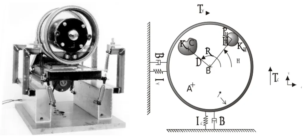
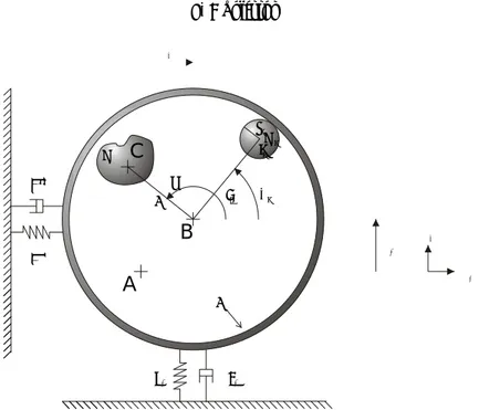
(12) CHAPTER 2. AUTOBALANCING. 4. x2 ri ii. mC c2. e. ωt. mi li αi. B k2. x1. n2 n1. A. M k1. c1. Figure 2.1: The left picture shows the experimental autobalancer equipped with two balance rings. Two balance rings are required to balance dynamic unbalance. Two compensating masses and the viscous media can also be seen. The right illustration shows the model used to analyze the autobalancer. By only using one balance ring placed at an approriate location on the axis, the experimental autobalancer is well described by the mathematical model found in equations 2.1-2.3.. The history of autobalancing is quite interesting in itself since it is not clear who the original inventor of the mechanism is. The person who is usually believed to be the inventor is E.L. Thearle, who …led a patent in 1934 describing its use to dynamically balance machine tools, see [38]. However, it has been told that this technique was used at the end of the eighteenth century to balance rotating parts in combustion engines. This was supposedly abandoned since it later became possible to manufacture rotating parts with little inherent imbalance.. 2.2. AutoBalancer. The cooperation between Electrolux and the Department of Mechanics resulted in a Master Thesis, see Adolfsson [1], where it is shown that good agreement between the theoretical model and experimental model is possible. Thus, it was decided to continue with the more speci…c parameter investigations. A detailed description of the theory behind autobalancing can be found in Adolfsson [2] (paper 1). In short, the idea is to have compensating masses, free to move in a circular path about the axis of rotation. At high enough rotational speed, these compensating masses will move to a position so as to reduce the vibration levels.

(13) 2.2. AUTOBALANCER. 5. in the system. The equations of motion used in all parameter studies are, i=n z }| { X M 0x Ä1 + c1 x_ 1 + k1 x1 = me!2 cos(!t) + mi li (Ä ®i sin(®i ) + ®_ 2i cos(®i )); (2.1) i=1. i=n }| { X z M 0x Ä2 + c2 x_ 2 + k2 x2 = me! 2 sin(!t) + mi li (Ä ®i cos(®i ) ¡ ®_ 2i sin(®i )); (2.2) i=1. (mi +. Ii )l ® Ä ri2 i i. + li (± i +. °i )(®_ i ri2. ¡ !) = mi (Ä x1 sin(®i ) ¡ x Ä2 cos(®i )). (2.3). i = 1; : : : ; n;. where the parts corresponding to a simple rotating unbalance are identi…ed, see Figure 2.1 or Table 1 and 2 for a description of the parameters and state variables. Table 1. Description of the parameters found in the autobalancing system. Parameter. M0 k1;2 c1;2 m e mi Ii ri li ±i °i !. Description Total mass of the system Spring constant in vertical and horizontal direction Viscous damping constant in vertical and horizontal direction Mass of unbalance Distance from axis of rotation to c.m. of unbalance Mass of compensating mass Moment of inertia of compensating mass Radius of the compensating mass Distance from axis of rotation to c.m. position of compensating mass Viscous damping constant - translation of compensating mass Viscous damping constant - rotation of compensating mass Angular velocity of the rotation system. Table 2. Description of the states found in the autobalancing system. State. x1;2 x_ 1;2 x Ä1;2 ®i ®_ i ® Äi. Description Horizontal and vertical position of the axis of rotation Horizontal and vertical velocity of the axis of rotation Horizontal and vertical acceleration of the axis of rotation Angular position of c.m. of compensating mass, measured relative to unbalance Angular velocity of compensating mass Angular acceleration of compensating mass.

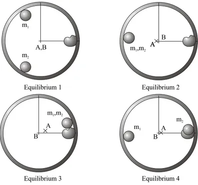
(14) 6. CHAPTER 2. AUTOBALANCING. Many of the questions answered in Adolfsson [2] (paper 1) are a result from phenomena discovered when working with the experimental autobalancer, and talking with the persons who built the autobalanced washing machine at Electrolux Wascator. For example, the operation of autobalancers requires some viscous media, typically oil, to operate. Due to varying temperature in washing machines, this oil might change its viscosity, potentially resulting in a failure of the autobalancer. Therefore, many of the parameter studies deals with studying the e¤ects of varying the parameters sensitive to temperature changes. Another important questions is what happens when the autobalancer is anisotropically suspended. Typically, a washing machine is suspended in a way that results in di¤erent sti¤ness in the horizontal and vertical directions. For example, it is shown that given enough separation in the horizontal and vertical natural frequency, autobalancing operation is possible in regions between these two frequencies. Generally, autobalancers require at least two compensating masses to function at varying amounts of unbalance. When using metal balls in a race the con…guration where all metal balls are lined up side by side corresponds to the maximum imbalance load that the system is capable of balancing. By …lling half the race with metal balls the maximum imbalance load is maximized. Adding an additional metal ball will only compensate for an already present metal ball. Thus, using only two metal balls in a race is usually not volume e¢cient since there is always the possibillity of using many smaller metal balls, which will reduce the volume occupied by the race. However, using more than two compensating masses complicates the parameter studies, since a family of equilibriums will result. Hence, the stability of the family of equilibrium positions have to be scanned for safe operation. Fitting an autobalancer on a rigidly mounted ‡exible shaft will result in equal sti¤ness in all directions. In this isotropic case, it is shown that the equations of motion 2.1-2.3 can be transformed to a time independent form, thus reducing the complexity of stability calculations and reducing the computational cost. Most studies on the autobalancer were carried out by linearizing the equations of motion about the di¤erent equilibrium positions existing in the system. This was done to …nd out their stability characteristics. For safe and robust operation it is important that the equilibrium, corresponding to a balanced system, is globally attractive. Since the autobalancer is capable of continuously adjusting to di¤erent imbalance loads, it is important that all imbalance loads result in stable equilibriums. However, this is not always case, and could lead to a problem if not all imbalance loads are tested in a real system. After it has been established that all imbalance loads result in a stable balanced equilibrium, it is important to investigate that these equilibriums are globally attractive. This was checked in three di¤erent systems by performing 30000 simulations, with random initial conditions and random imbalance load. The investigated systems have the same capacity, in terms of imbalance load, but are con…gured di¤erently. The …rst system have heavy compensating masses close to the axis of rotation and the last two have lighter compesating masses far from the axis. Histograms are presented showing the number of revolutions before the system.

(15) 2.3. CONCLUSION. 7. is satisfactorily balanced. The general result indicates that when the desired equilibrium positions are stable, they are also globally attractive. However, the system with the heavy compensating masses close to the axis balance the system faster than the other two. The local stability of the three systems are also compared and it appears like the local stability can be used as reasonable guide to optimize the system. Other studies on autobalancing systems have been done by for example Hedaya et al. [12], which report similar stability results when internal and external damping are varied. These studies have been performed on a system similar to a washing machine. Friction e¤ects and a study of the e¤ects of the eccentricity of the race have been done by Majewski [25] and [26]. In reference [9], Bövik et al. shows that it is possible to have autobalancing in non-plane rotors by using multiple scale techniques. It is also interesting to note that some early theoretical studies, using simpli…ed models, had come to certain conclusions regarding stability and rotational speed. These result do not seem to agree with experiments and more advanced models, see Kravchenko [18],[20], and [19].. 2.3. Conclusion. There still isn’t any widespread use of autobalancing technology, which might be explained by the one big disadvantage of autobalancers. Namely, that they don’t work at rotational speeds lower than the lowest natural frequency of the system, see Adolfsson [2] (paper 1). Sometimes, it can even be disadvantageous to have an autobalancing system at low rotational speeds. Many devices have been developed to overcome this problem, such as clamping the compensating masses at low speeds, only releasing them at high speeds. However, introducing these locking devices removes the attractive simplicity of the mechanism and certainly increase its cost. Despite this, SKF, with its long history of making ball bearings, have developed autobalancing into a commercial product named DynaSpin, see [36]. They envisage use in washing machines, grinders, centrifuges, and optical storage devices. It will be interesting to see if they succeed in making autobalancing a successful commercial product..

(16) 8. CHAPTER 2. AUTOBALANCING.

(17) Chapter 3. 3D Passive Walking 3.1. Background. The activity of normal walking is something we perceive as requiring very little conscious e¤ort. While on a higher level it is clear that some sort of control is necessary, such as that required for negotiating rough terrain and recovering from large disturbances, on a lower level it has been shown that the ability to walk is largely a consequence of the inertial and geometrical makeup of bipedal mechanisms, see Basmajian and Tuttle [8] and McGeer [28], [27], [29]. The models studied in this paper are usually referred to as passive walkers, see McGeer [28], since the source of energy is gravity alone and no external active control is applied. Sustained gait is realized by letting the walker descend an inclined plane to counteract the energy dissipated in collisions with the ground and in the knees. To accomplish walking on level ground, actuation would be needed. Di¤erent schemes for actuation have been thought of using for example a leaning torso as to provide a torque on the upper legs, see Howell and Baillieul [14] or impulsive pushing of the hind legs, see McGeer [30]. Most of the previous studied passive walkers have been constrained to move in a plane to prevent lateral dynamics. However, to be successful in a life like environment it is evident that a fully three dimensional walker is needed. Many successful attempts have been made to build active walking mechanisms. The most successful up to date is the Honda Biped [13]. This walker is capable of walking in relatively life like environments, such as climbing stairs. The P1 version weighs about 210kg and can operate for about 10 minutes on its own battery pack. The position of limbs are controlled using electrical direct drive servos. Since electrical motors usually have low torque and high speed, some sort of gearing is necessary. This gearing both ampli…es inertia and friction, thus making it hard to control the actual force output on the limbs. Instead, it is most common to control the position and angle of di¤erent joints. The drawback of this is that it makes it hard to use the natural dynamics available to the mechanism, such as the natural pendulum motion of a swinging leg. In light 9.

(18) CHAPTER 3. 3D PASSIVE WALKING. 10. Rolling foot to point foot. Extending the toe point to a line toe. Separating the hip. No overlap in the feet. Figure 3.1: The steps taken to extend the planar passive walker into a 3D passive walker. of this, we decided to try to extend the planar passive walker into a fully three dimensional passive walker, having dynamics in all spatial directions. The idea was to slowly extend previous found planar walkers into a three dimensional con…guration, see Figure 3.1. The planar passive walker, originally devised by McGeer [27], had large radius feet and attempts to directly extend this con…guration into three dimensions had resulted in unstable dynamics of the system, McGeer [30]. Other attempts had succeeded, albeit outside the passive category by using active control to stabilize the swaying motion, Kuo [21]. The …rst successful experimental attempt was the passive and knee-less Tinkertoy walker, see Coleman et al. [10], which was later modeled and shown stable, Mombaur et al. [10] [32]. However, it requires masses to be put on extended booms as to obtain the necessary moments of inertia. The path taken here was to add an extra contact point to the foot. This was made possible after realizing that the foot radius could be shrunk to zero, see Adolfsson and Nordmark [5] (paper 3). By starting with very wide feet, see Figure 3.1, the dynamics would essentially resemble those of the planar walkers. Thus initial conditions and parameters from the planar walker could be utilized. The extension into three dimensions resulted in a lot of new dynamics such as gaits heading obliquely down the plane, see Dankowicz et al. [11] (paper 6) and Piiroinen et al. [33] [34]. The initial extension was made using direct numerical simulation. Thus, the convergence to periodic gaits were slow. Therefore, a root …nding algorithm was developed to locate periodic gaits, see Adolfsson et al. [6] (paper 5) and Adolfsson [3] (paper 7). This also made it possible to locate unstable periodic gaits. The reason for studying unstable gaits is that they can turn into stable gaits as parameters of the system are varied. Potentially, …nding new stable gaits, which would have been hard or impossible to locate using direct numerical.

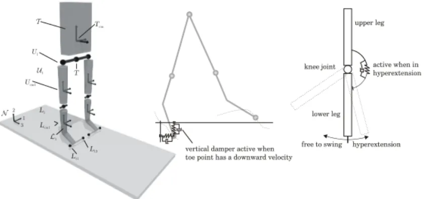
(19) 3.2. 3D PASSIVE WALKER. T. 11. upper leg. Tcm. U1 U1. knee joint. T. active when in hyperextension. Ucm1. N. L1. 2 1 3. lower leg. Lcm1 L1 L12 L11. vertical damper active when toe point has a downward velocity. free to swing. hyperextension. Figure 3.2: The di¤erent bodies of the 3D passive walker. Continuous impact dynamics are used in knee and ground plane. simulation. Initial attempts with the root …nding algorithm looked promising and work started on …nding a 3D passive walker having no overlap in the feet and a geometry resembling a human, see Adolfsson [4] (paper 8).. 3.2. 3D passive walker. The mechanical model of the walker consists of …ve rigid bodies connected by hinge joints, as depicted in Figure 3.2. The bodies are the torso, the upper legs, and the lower legs. The walker makes regular contact with the ground plane through its four toe points. The 3D passive walker is modeled as a continuous system, where the impact laws used for the planar walker have been replaced by springs and dampers. These are activated based on the state the walker is in, such as knee-lock and contact with ground, thus avoiding the complexity of treating di¤erent impact sequences. A problem that could occur if impact models were used is that the toe points, representing the contact cylinder, could bounce between its ends in…nitely many times in a …nite time. To handle this would require some extra conditions on the impact models. Thus, the interaction between walker and ground plane is through springs and dampers attached from the initial toe contact point to the toe points. These springs/dampers are active as long as the toe point is below the ground plane, see right pane of Figure 3.2. In human walking, the stance-leg knee is never overstretched. Instead muscles prevent the knee from collapsing, see Inman et al. [15]. To prevent a collapse of the knee in our model, the knee has to be in hyperextension where it rests against a torsional spring/damper. For a detailed description on geometry, kinematics, and forces/torques acting on the walker see Adolfsson et al. [6] (paper 5) and Adolfsson [3] (paper 7)..

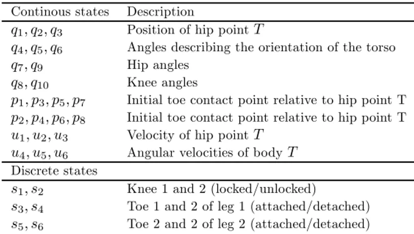
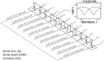
(20) CHAPTER 3. 3D PASSIVE WALKING. 12. Table 3. Continous and discrete state variables.used in the 3D passive walker Continous states. q1 ; q2 ; q3 q4 ; q5 ; q6 q7 ; q9 q8 ; q10 p1 ; p3 ; p5 ; p7 p2 ; p4 ; p6 ; p8 u1 ; u2 ; u3 u4 ; u5 ; u6. Description Position of hip point T Angles describing the orientation of the torso Hip angles Knee angles Initial toe contact point relative to hip point T Initial toe contact point relative to hip point T Velocity of hip point T Angular velocities of body T. Discrete states. s1 ; s2 s3 ; s4 s5 ; s6. Knee 1 and 2 (locked/unlocked) Toe 1 and 2 of leg 1 (attached/detached) Toe 2 and 2 of leg 2 (attached/detached). Table 4. Description of the parametrization of the 3D walker. Body Torso Upper legs Lower legs Hip joints Knee joints Toe points Knee dynamics Hip damping Ground plane Inclination. 3.3. Parameter description Described by a center of mass position, a mass, and six moments of inertia See above See above Position on hip line Relative to hip joint in upper leg direction Each toe point is described by three coordinates, two toe points on each leg A angular knee sti¤ness and damping To resist rotations of the torso Sti¤ness and damping in three directions Inclination of the ground plane Total. nr. 10 10 10 1 1 6 2 1 6 1 48. Numerical simulation. In Figure 3.3, a stick animation of the 3D walker is shown, sampled at the di¤erent events for twelve consecutive gait cycles. This particular walker has an overlap in the feet of 0.1m. The walker is started just after the impact of the right leg’s toe points. The events for each toe of the legs are combined into one stick …gure, since the time interval between the successive impacts or successive releases is very short. The event percentage is de…ned relative to the stride.

(21) 3.4. FINDING AN IMPLEMENTABLE 3D PASSIVE WALKER. 13. Hip center motion. Height (m). 0.67. 0.64 -0.02. 0. 0.02. Lateral deflection (m). Stride time 1.6s Stride length 0.69m Inclination 4.6°. Figure 3.3: Stick animation of an stable periodic gait of the 3D walker. Toe clearance refers to the con…guration having a nonzero local minimum in distance between toe points and the ground plane. time. With methods described in Adolfsson et al. [6] (paper 5) it can be shown that this choice of parameters and initial conditions result in an stable periodic gait.The butter‡y-shaped orbit of the center of the hip, as displayed in Figure 3.3, shows a similarity with results reported in Rose and Gamble [35].. 3.4. Finding an implementable 3D passive walker. Initial attempts to reduce the foot overlap to zero resulted in unstable periodic gaits, see Adolfsson et al. [6] (paper 5). Thus, an extensive parameter search was undertaken to …nd a walker without an overlap. The 3D passive walker is described by 28 state variables and approximately 80 parameters. If the left and right side of the walker are mirrored in the sagittal plane, the number of parameters will be reduced to 48, see Table 4. The sheer number of parameters makes it hard to draw any reasonable conclusions about a particular parameter variation. Typically, the conclusion drawn from a one parameter variation might not hold if one changes the value of another parameter. This emphasizes the importance of having a very clear goal when performing parameter studies, such as …nding an implementable 3D passive walker. Below are the requirements set up for an implementable 3D passive walker. ² The mass distribution should be realizable, thus masses should not have to be placed in awkward positions, such as on long extended booms, to get the required moment of inertia. ² Required friction between toe points and ground plane should be reasonable..

(22) CHAPTER 3. 3D PASSIVE WALKING. 14. ² There should be an anthropomorphic (human like) look of the 3D passive walker. This means that geometrical measures of the experimental walker should have similar ratios as a human. For example, the ratio of leg length to hip width should be close to the values found in humans. ² No overlap of the feet. ² Insensitive to parameter changes. This is especially important when the parameters are hard to control or measure in an experimental walker. For example, the actual force between ground and toe points might be very hard to model. Thus, a stable gait should exist for reasonable intervals in the parameters associated with the ground plane. ² Initial conditions that is possible to realize and have a reasonable basin of attraction. The latter might be hard to investigate due to the number of states of the walker. ² Be able to carry some payload, however not necessarily with an upright torso, which most likely would require active control. ² Knee mechanism should be possible to implement passively. The current design requires quite large angular motions of the lower legs during the locked state of the knees. The search to ful…ll these requirements and a presentation of the implemented 3D walker are given in Adolfsson [4] (paper 9).. 3.5. Conclusion. It is believed that most of these requirements were ful…lled during the parameter search. However, we were not able to achieve a stable working walker in the laboratory. There are two possible reasons for this, the parameters of the experimental walker didn’t match the parameters used in simulation or the walker was not started in the basin of attraction of found stable gaits. It could also be that it was a combination of these two reasons. But due to the lack of adequate measuring equipment, such as 3D motion measuring system, it is hard to know why it failed. For a more thorough discussion on why it failed and possible suggestions to make it work, see Adolfsson [4] (paper 9). Despite this, it is believed that the results presented here still support the assumption that human gait is largely a consequence of geometry and mass characteristics..

(23) Chapter 4. Mechanics To calculate the motion of a rigid body we use Newton’s equation or the linear momentum principle N. d (mv) = F; dt. (4.1). where N is the inertial reference frame where the time derivative is taken, v is the body center of mass velocity given in the inertial reference frame N , and F is the external force acting on the body. Together with the mass center motion, we also need to know how the orientation of the body evolves in time, which is governed by the angular momentum principle N. d (L) = T; dt. (4.2). where L is the angular momentum of the body and T is the torque acting on the body. Its interesting to note that equation 4.1 and 4.2 does not contain any explicit dependence on the actual position or orientation of the body. This is obvious in equation 4.1, and can be seen in the latter equation by carrying out the di¤erentiation of the angular momentum N. N B d d d (L) = (I!) = ! £ I! + I (!); dt dt dt. where both the angular velocity vector ! and the moment of inertia dyad I are expressed in the reference frame B attached to the body. However, most forces and torques acting on bodies depends on both position and orientation. Some of these forces might be a result of constraints applied to the body. Constraint forces/torques play an important role since they can be viewed as control systems, operating on a much smaller time scale than the rest of the system as to maintain the constraints. Constraints can typically be divided into position/orientation constraints and velocity constraints. All position/orientation constraints (holonomic constraints) can be turned into velocity constraints through di¤erentiation, however not all velocity constraints 15.

(24) CHAPTER 4. MECHANICS. 16. can be turned into coordinate constraints. These, non-integrable constraints are called non-holonomic constraints. Examples of holonomic constraints are; hinges, joints, and guides. Examples of non-holonomic constraints are a skate on ice or a sphere rolling on a plane. Constraints on a mechanism results in forces/torques, therefore one usually divide the right hand side of equations 4.1 and 4.2 into F = FC + FA and T = TC + TA. (4.3). where the division between constraint and applied forces/torques has been made. Various methods have been developed to either remove or calculate these constraint forces from the equations of motion, such as for example Lagrange’s method and Kane’s method which removes the constraint forces/torques and di¤erential algebraic formulations which calculates them. Naturally, all these techniques result in the same dynamics. However, Kane’s method has proven to be practical in deriving equations of motions for engineering systems where the number of bodies and constraints are not too high. The method of …nding the equations of motion and stating the constraint forces can be viewed as a two step process. We start by describing the position and orientation of our bodies using generalized coordinates qi : For free and unconstrained bodies this would require six generalized coordinates for each body. If we have simple constraints, such as hinges, joints and guides and the mechanism does not have any closed loops, it is usually possible to describe the con…guration by using a minimum set of generalized coordinates. Since this is not always possible the second step is therefore to state the additional contraints as relations between the generalized coordinates or its time derivative, the generalized velocities. Thus, by using generalized coordinates qi we can express the position xj and orientation Rj of our bodies as xj Rj. = xj (q) and = Rj (q). (4.4). where the index j runs over the bodies. By di¤erentiation of these relations we obtain a linear relation between our generalized velocities q_i and the physical velocities vj and !j ; 2 T 3 v1 6 ! T1 7 _ (4.5) 5 = A(q)q: 4 .. . where the columns of A is a set of basis vectors for the possible motions of the system. D’Alembert’s principle of ideal constraints now says that the forces/torques acting on the bodies can be written as 1 0 ¢ ¢ ¢ ¹1 b1 ¢ ¢ ¢ C X B [Fb1 ; Tb1 ; ¢ ¢ ¢ ] = @ ¢ ¢ ¢ ¹2 b2 ¢ ¢ ¢ A = ¹i bi = ¹B; .. i ..

(25) 17 where B should satisify BA = 0 and the scalars ¹i (t) can be determined. The additional constraints we might have can be described as relations between the generalized coordinates of the mechanism. Thus they can be written as fi (q) = 0: By di¤erentiating these constraints with respect to 0 ¢¢¢ X @fi @fi B ¢¢¢ q_k = 0; Cik = =@ @qk @qk k. time, we get, 1 c1 ¢ ¢ ¢ c2 ¢ ¢ ¢ C A: .. .. If we have additional velocity constraints, they can also be added to Cij . The null space of matrix Cij now represents a subspace of possible motions of the system. A set of basis vectors of this subspace is usually referred to as the tangent vectors ¿ i , 1 0 .. .. . . C B C C(q)¿ (q) = 0; where, ¿ = B @ ¿ 1; ¿ 2; ¢ ¢ ¢ A : .. .. . . The velocity con…guration of the mechanism can be written in the tangent base as, q_ = ui ¿ i. (4.6). where the scalars ui are the coordinates in this base and are named generalized speeds. Our physical tangent vectors ¯i can be written as ¯i = A¿ i by using equation 4.5 in 4.6. D’Alembert’s principle now states that the projection on A of the constraint forces/torques resulting from these constraints can be written as X ¸i ci = ¸C [Fc1 ; Tc1 ; ¢ ¢ ¢ ] A = i. where ¸i (t) are scalars. Taking the dot product between our physical tangent vectors ¯i and the constraint forces/torques will result in ¢ £ C C ¤ ¡£ b b ¤ F1 ; T1 ; ¢ ¢ ¢ ¯ = F1 ; T1 ; ¢ ¢ ¢ + [Fc1 ; Tc1 ; ¢ ¢ ¢ ] ¯ = ([¢ ¢ ¢ ] + [¢ ¢ ¢ ]) A¿ = (¹BA + ¸C)¿ = 0:. Thus, by making the division between applied and constraint forces/torques in the right hand side of Newton’s equation and the angular momentum principle we get N. d C A c b (mj vj ) = FA j + Fj = Fj + Fj + Fj and dt N d C A c b (Ij !j ) = TA j + Tj = Tj + Tj + Tj : dt. (4.7) (4.8).

(26) CHAPTER 4. MECHANICS. 18. Now, the dot product between the constraint forces/torques and the physical tangent vectors will vanish. Thus, we can take the dot product on the right hand side and left hand side of equation 4.7 and 4.8 to get rid of the constraint forces/torques ·µ N ¶ µN ¶ ¸ d d A A (m1 v1 ) ¡ F1 ; (I1 !1 ) ¡ T1 ; ¢ ¢ ¢ ¢ ¯i = 0; dt dt which result in one equation for each ¯i .. 4.1. Sophia. Sophia is a tool for deriving equations of motion and follows Kane’s method; see Kane & Levinson [17]. Sophia, originally developed by Lesser [24] and [23], runs in computer algebra programs such as Maple and Mathematica. It contains tools for handling reference frames, rotations, frame-based di¤erentiation, computing tangent vectors, and an implementation of Kane’s method. An export utility, exmex has been developed by Lennartsson [22], which provides functionality for exporting equations of motion for numeric integration in Matlab. It also provides support for forming and exporting variational equations of dynamical systems, which can be used in stability calculations. The extension to multi-body dynamics is done via a construct called Kvectors, which is a list of ordinary vectors. The velocity con…guration K-vector contains the center of mass velocities and angular velocities of each body, 2 3 v<1 6 ! <1 7 6 7 6 7 v< = 6 ... 7 6 7 4 v<K 5 ! <K. A similar construct is used to hold the corresponding applied forces/torques on each body in the system, 2 3 F<1 6 T<1 7 6 7 6 .. 7 R< = 6 7: a 6 . 7 4 F<K 5 T<K. By expressing the system velocity con…guration v< using a minimum set of generalized speeds ui , it is possible to extract the tangent vectors, since v< can be written as X < ui ¯< v< = i + ¯ (t): i.

(27) 4.1. SOPHIA. 19. Momentum and angular momentum is obtained by multiplying each row in v< by either the mass mi or the moment of inertia dyad Ii ; 2 3 m1 v<1 6 I1 ! <1 7 6 7 6 7 .. P< = 6 7; . 6 7 4 mK v<K 5 IK ! <K. where K is the number of bodies. Using D’Alembert’s principle it is now possible < to get rid of the constraint forces/torques since R< c ² ¯ i = 0, where the fat dot product is an operation where the ordinary dot product between vectors is performed between each row and the result is summed up. By using these tangent vectors on Newton’s equations and the angular momentum principle one gets < _ < ¡ R< (P a ) ² ¯ i = 0;. which results in as many equations as there are ¯< i ’s. These equations, together with the KDE’s, usually on the form q_i = Wij (q)uj ; can be retained on an implicit form or can put on a …rst order form, q_i u_ i. = gi (q; u); = hi (q; u; t);. since the equations motion are linear in all derivatives. These …rst order form equations are suitable for numerical integration in standard ODE packages..

(28) 20. CHAPTER 4. MECHANICS.

(29) Chapter 5. Analysis methods 5.1. Nonlinear dynamics. Generally, it is not possible to analytically solve nonlinear ordinary di¤erential equations (nonlinear ODEs). We therefore have to resort to numerical methods. Today, it exists many robust integrators, capable of handling di¤erent types of ODE’s. In this thesis, all integration has been performed using Matlab’s ODE suite, which range from non-sti¤ to sti¤, low-order to high-order, and variableorder integrators. A general nonlinear dynamical system is described by a set of di¤erential equations having a nonlinear driving function, this can be written as x_ = f (x):. (5.1). If the system doesn’t explicitly depend on time it is said to be autonomous, otherwise it is said to be non-autonomous. Points x¤ for which f (x¤ ) = 0 are called equilibrium points of the system. If the system is started at an equilibrium point, it will stay there and x(t) = x¤ for all times. If all neighboring points are attracted to this point, it is said to be stable. If some neighboring points are repelled, it is said to be unstable, see Figure 5.3 for an illustration of this. Depending on the complexity of the equations of motion, it can sometimes be convenient to put the equations of motion in the form: M (x; t)x_ = g(x; t); where f = M ¡1 g:. (5.2). This is useful when an explicit inversion of M(x; t) is cumbersome.. 5.1.1. Flow. Although it is not possible to generally write a closed form solution to equation 5.1, we can, given the initial condition x(0) = x0 , formally de…ne the ‡ow of 21.

(30) CHAPTER 5. ANALYSIS METHODS. 22. solutions x(t) = ©(x0 ; t) where © satis…es @© = F (©) and @t ©(x0 ; 0) = x0 :. 5.1.2. Limit cycles. In nonlinear systems, self-sustained oscillations can occur, such as the famous Van der Pol oscillator, see José and Soletan [16]. These self-sustained oscillations are called limit cycles and are isolated and closed trajectories of the dynamical system. Thus, in terms of the ‡ow a limit cycle has to ful…ll ©(x; t) = ©(x; t + T ); where T 6= 0 is the period time of the limit cycle. The periodic gait of the passive walker is a limit cycle, since the walker returns to the same con…guration, having the same velocities, after one stride. Stable limit cycles attract neighboring trajectories, thus if the stable limit cycle is slightly perturbed, the system will asymptotically return to the original limit cycle. Conversely, unstable limit cycles repel some neighboring trajectories.. 5.1.3. Stability of the dynamical system. Stability of the equilibrium point x¤ can be calculated by linearizing the nonlinear dynamical system found in equation 5.1 about the equilibrium point. For a proof that linearization works for hyperbolic equilibrium points, Strogatz [37] gives a reference to Andronov et al. [7]. Introduce a small displacement 4x from x¤ and Taylor expand the right hand side of equation 5.1 _ = f (x¤ ) + (x_ ¤ + 4x). @f 4x + O(j4xj2 ): @x. However, for an equilibrium point x_ ¤ = f (x¤ ) = 0 and we are left with 4x_ =. @f 4x; @x. neglecting higher order terms. The matrix @f =@x is called the Jacobian of the system and controls how small disturbances about the …x point evolve in time. The general solution to this linear di¤erential equation is (assuming no repeated eigenvalues of the Jacobian) X 4x(t) = ®i vi e¸i t i. where ¸i are the eigenvalues of the Jacobian, vi are the corresponding eigenvectors, and ®i are determined by 4x(0). Hence, 4x(t) will tend to zero if the real part of all ¸i s are less than zero. Thus, the equilibrium point is stable if all eigenvalues have a real part less than zero..

(31) 5.1. NONLINEAR DYNAMICS. 23. xk xk+1. xk+2 x*. Figure 5.1: Consecutive intersections of the Poincaré section H(x) = 0 by a trajectory of the dynamical system: The limit cycle starts and ends in the same point x¤ of the Poincaré section.. 5.1.4. Stability of limit cycles. This method is …ne as long as we have equilibrium points of the dynamical system, but what about limit cycles? To study their stability we introduce a Poincaré surface/section H(x) = 0 into the ‡ow that the limit cycle intersects transversely, see Figure 5.1. Thus, we can now look at the consecutive points of intersection of this surface. This is called a Poincaré map, xk+1 = f (xk );. (5.3). if all xk belongs to the surface and the intersection xk of this surface is followed by the intersection xk+1 . If we start with a point on the limit cycle and in the Poincaré section, the same point will be intersected turn after turn, x¤ = f (x¤ ), x¤ is said to be a …xed point of the Poincaré map. We are now interested to see how points close to this …xed point map. Introduce a small disturbance d0 and Taylor expand the right hand side of equation 5.3 about the …xed point, x¤ + d1 = f (x¤ + d0 ) = f (x¤ ) +. @f d0 + O(jd0 j2 ): @x. However, x¤ = f (x¤ ); since x¤ is a …xed point, and the result is, d1 =. @f d0 ; @x. or more generally, dk+1 =. @f dk : @x.

(32) CHAPTER 5. ANALYSIS METHODS. 24. In a similar fashion to the vector …eld case, @f =@x is said to be the Jacobian of the linearized Poincaré map for the …x point x¤ . Asymptotic decay to x¤ of all neighboring points is assured as long as the eigenvalues of the Jacobian are all inside the unit circle. This stability criterion can easily be seen if we assume that Jacobian has no repeated eigenvalues. If so, we can express the initial disturbance d0 using the eigenvectors of the Jacobian, X d0 = ®i vi : i. Inserting this into the linearized Poincaré map we get, d1 =. @f X ®i vi : @x i. Since the vi ’s are the eigenvectors of Jacobian and therefore @f =@xvi = ¸i vi . This results in X (¸i )k ®i vi ; dk = i. and as long as all j¸i j < 1; dk will tend to zero as k goes to in…nity.. 5.1.5. Finding limit cycles. Much of the work relating to …nding an implementable 3D passive walker has been focused on …nding periodic gaits. Since periodic gaits of the walker correspond to limit cycles of the dynamical system a method of locating limit cycles has been implemented. The problem of …nding limit cycles can be stated as that of …nding x0 and T0 6= 0 satisfying ©(x0 ; T0 ) ¡ x0 = 0:. (5.4). However, the number of unknowns exceeds the number of equations by one (all points on the limit cycle ful…ll equation 5.4 above), so a Poincaré section is used to make the solution locally unique, H(x0 ) = 0: If we now have a good initial approximation (x0 ; T0 ) to the solution of the above we can calculate an update (4x; 4T ) that will take us closer to the solution by using the Newton-Raphson method, ¸ ¸· · ¸ · ¢x ©(x0 ; T0 ) ¡ x0 @x ©(x0 ; T0 ) ¡ I @t ©(x0 ; T0 ) =¡ (5.5) ¢T @x H(x0 ) 0 H(x0 ) where I is the identity matrix, see Adolfsson [6] (paper 6)..

(33) 5.2. BIFURCATIONS. 5.1.6. 25. Variational equations. The derivative of the ‡ow @x ©(x0 ; T0 ); found in equation 5.5, can be obtained through the standard variational equations, see Adolfsson et al. [6] (paper 6). Forming and exporting the variational equations to Matlab code is supported by the exmex package, see Lennartsson [22]. This includes support for using implicit formulations, as in equation 5.2, or explicit formulations, as in equation 5.1.. 5.1.7. Discontinuities. Di¤erent types of discontinues can be encountered in engineering systems. For example, force discontinues occur if the Coulomb friction model is used or if a particle goes from one media to another, such as a particle impacting with a water surface. Discontinuities involve the sudden change of state variables and/or their derivatives. This typically occurs in standard impact models, where velocities of the system change discretely according to some impact model. In the 3D passive walker, force discontinues occur when the knee locks or when the foot impacts with the ground. Sudden change of state variables also occur, since the initial foot contact point is stored as a state of the system. Thus, it is discontinuously updated at each foot impact. The standard use of variational equations has to be suitably modi…ed at a discontinuity. Although a little bit intricate to derive, see Müller [31] or Adolfsson et al. [6] (paper 6), the resulting discrete Jacobian correction has a simple form ª = @x G +. (Fa ¡ @x GFb )@x N ; @x N Fb. where Gi!j is the discrete change in state variables, Fa and Fb is the vector …eld of the dynamical system just after and just before the discontinuity, and @x N is the normal of the impact surface, see Figure 5.2 for an illustration. Applying this discrete Jacobian correction to the derivative of the ‡ow just before the discontinuity will yield the derivative of the ‡ow just after the discontinuity, @x ©after = ª@x ©before :. 5.2. (5.6). Bifurcations. Bifurcations occur when the stability type of the system is changed. The stability type of the system might change as parameters are varied. The parameter value where the system changes stability type is called a bifurcation point. Here, we assume that the crossing occurs transversely. Thus, if we are looking at the variation of a parameter ¹; we assume that ¯ @ Re(¸) ¯¯ 6= 0 @¹ ¯Re(¸)=0.

(34) CHAPTER 5. ANALYSIS METHODS. 26. N(x)=0 G(x). ©(x,t) Nx. Fb. Fb. Figure 5.2: A trajectory of the dynamical system intersects a discontinuity surface N (x) = 0 where the state variables are updated to a new position in state space by the function G(x): The vector …eld is given by Fb at the intersection of the discontinuity surface and Fa at the new updated position. unstable equilibrium. no equilibrium. unstable equilibrium. stable equilibrium stable equilibrium. stable equilibrium. stable equilibrium. Figure 5.3: A bifurcation occurs when a system changes its stability type. Assume that the spheres move on a surface that is lowered into some viscous media. The equilibrium position of the left bowl will be stable. If the bowl is gradually transformed into the right bowl, the middle position will loose its stabillity and two new stable equilibrium positions are created. This is called a pitchfork bifurcation. The incline illustrates a saddle node bifurcation. No equilibrium exist in the left incline and as it is gradually changed into the right incline, one stable and one unstable equilibrium is created.. for an equilibrium point in a dynamical system and that ¯ @ j¸j ¯¯ 6= 0 @¹ ¯j¸j=1. for a …xed point of the Poincaré map. Two di¤erent types of bifurcations are illustrated in Figure 5.3, where the stability of a small particle on an incline and in a bowl are shown. The two bifurcations that are illustrated are the saddle-node bifurcation and a super-critical pitchfork bifurcation, however there exists other bifurcations. The bifurcations occurring in the two studied systems are described below. Since stability criterions are di¤erent for equilibrium points of the dynamical system and …xed points of the Poincaré map, they are listed separately..

(35) 5.2. BIFURCATIONS. 5.2.1. 27. Saddle-node bifurcations. Saddle-node bifurcations occur in the passive walker system as the inclination is decreased. At some inclination one stable and one unstable branch are created. This bifurcation also occur in the autobalancer, for some of the equilibrium positions, as the rotational speed is varied. Flow: A real valued eigenvalue starts at 0 and either goes to the left half plane (stable branch) or goes to right half plane (unstable branch). Poincaré map: A real valued eigenvalue starts at 1 and either becomes less than 1 (stable branch) or greater than 1 (unstable branch).. 5.2.2. Pitchfork bifurcations. These bifurcations usually occur in systems with symmetry. The 3D walker has a right and left symmetry with respect to the legs. It is the super critical pitchfork bifurcation that usually occurs in the 3D walker. Typically, the gait heading straight down the plane becomes unstable and two oblique gaits emerge. These two oblique gaits are mirrored in each other, see Piiroinen et al. [33]. This bifurcation has not been observed in the autobalancer due to the lack of symmetry. Flow: A real valued eigenvalue crosses the border between the right and left half plane. Poincaré map: A real valued positive eigenvalue goes through the unit circle. If the two forked solutions are stable, a super critical pitchfork bifurcation is said to occur, if the two forked solutions are unstable a sub critical pitchfork bifurcation is said to occur. The forked stable solutions always occur on the unstable side and vice versa.. 5.2.3. Hopf bifurcations. Hopf bifurcation occurs both in the autobalancer and the 3D walker system. A super critical Hopf bifurcation occurs in the autobalancer if the damping on the compensating masses is decreased or if the suspension damping is increased. The result is small oscillations of the compensating masses. Flow: A complex conjugate eigenvalue pair crosses the border between the right half plane and left half plane. Poincaré map: An eigenvalue pair crosses the unit circle. If there exist a small stable limit cycle on the unstable side, a super-critical Hopf bifurcation is said to occur, the amplitude of this oscillation is proportional to the square root of the distance from the bifurcation point. The sub-critical Hopf bifurcation occurs if there exist a small unstable limit cycle at the stable side. In engineering the sub-critical bifurcation is the most dangerous of the two types, since no stable limit cycle is available after the bifurcation has occurred..

(36) CHAPTER 5. ANALYSIS METHODS. 28. 5.2.4. Period doubling. Period doubling sequences occur in both systems analyzed in this thesis. In the autobalancer the previous mentioned limit cycles goes through a series of period doublings, eventually resulting in chaotic motion of the compensating masses. This occurs when the damping on the compensating masses are further decreased or if the suspension damping is further increased. In the 3D passive walker this sometimes occurs when varying the inclination of the plane. It always occurs after a pitchfork bifurcation has occurred, creating oblique gaits. Just after the period doubling has occurred, the limit cycle will take twice the time to return to the same point in the Poincaré map compared to before the period doubling. In the planar walker, a sequence of period doublings is typically followed by chaotic regions. Poincaré map: An eigenvalue goes through ¡1.. 5.3. Conclusion. In this thesis, the dynamics of two di¤erent mechanical models are explored using standard dynamical systems methods. The mechanical models are the autobalancer and the three dimensional passive walker. The two models differ in complexity and details but the analysis methods are similar. The model for the autobalancer results in a smooth dynamical system whereas the passive walker includes di¤erent kinds of discontinuities. These discontinuities are taken care of by introducing suitable mappings. In the case of the autobalancer it is possible to analytically solve for the time independent equilibrium positions. The equations of motion are then linearized about the equilibrium positions and stability can be assessed. It is not possible to analytically solve for the periodic gaits of the passive three dimensional walker. Hence, a Newton-Raphson root solving scheme for locating periodic gaits was implemented. Periodic gaits correspond to limit cycles of the dynamical system. Since this scheme involves integrating the variational equations of the ‡ow, stability is easily assessed after the root solving scheme has converged to an equilibrium point. The process of deriving analytical expressions for the equations of motion and the variational equations would not have been practical without symbolical manipulation programs. For example, the compiled C code for calculating the equations of motion of the passive walker are about 90kb and the variational equations is about 300kb. The methods described in this thesis are not limited to the study of autobalancing and passive bipedal walking but are applicable to many mechanical systems with or without discontinuities..

(37) 5.3. CONCLUSION. state. 29. saddle node pitchfork (super critical) pitchfork (sub critical) stable. hopf (super critical) unstable. hopf (sub critical) period doubling bifurcation point. parameter. Figure 5.4: Illustration of bifurcations occuring in the autobalancing system and the 3D passive walker system. The saddle node bifurcation is characterized by the sudden birth of two solutions, one stable and one unstable. The pitchfork bifurcation is characterized by the creation of two forked solutions at the bifurcation point. Pitchfork bifurcations come in two ‡avors, super- and sub-critical. Hopf bifurcations occur when small limit cycles are born at the bifurcation point. This type of bifurcation can also be sub- or super-critical. The …nal bifurcation discussed here is the period doubling. These might occur when limit cycles changes their stability in a certain way..

(38) 30. CHAPTER 5. ANALYSIS METHODS.

(39) Chapter 6. Acknowledgements I would like to express my gratitude to the people at the Department of Mechanics who have made it possible for me write this thesis. First o¤ all I would like to thank my advisor, Professor Martin Lesser for his support and advice. I would also like to thank Dr. Arne Nordmark for sharing his knowledge and insights in the …eld of dynamics and mechanics, Dr. Harry Dankowicz for awakening my interest in passive walking and the many valuable and insightful discussions about interpreting research results, and Dr. Anders Lennartsson is gratefully acknowledged for his export routines. It has also been a pleasure to work with Dr. Hanno Essén, Tekn. Lic. Petri Piiroinen, Dr. Mats Fredriksson, Gitte Ekdahl, my room-mate Per J. Olsson, and the colleagues and friends at the Department of Mechanics. Finally, I thank the members of my family and Helena, for their support.. Partial …nancial support from Volvo Research Foundation is gratefully acknowledged.. 31.

(40) 32. CHAPTER 6. ACKNOWLEDGEMENTS.

(41) Bibliography [1] Adolfsson, J.: 1995, ‘Self Balancing of Rotating Machines: An Experimental and Theoretical Study’. Master’s thesis, KTH, Department of Mechanics. [2] Adolfsson, J.: 1997, ‘A Study of Stability in Autobalancing Systems using Multiple Correction Masses’. Technical report, KTH, Department of Mechanics. [3] Adolfsson, J.: 2000a, ‘3D Passive walkers: Code Implementation Issues’. Technical report, KTH, Department of Mechanics. [4] Adolfsson, J.: 2000b, ‘Finding an Implementable 3D Passive Walker using Continuation Methods’. Technical report, KTH, Department of Mechanics. [5] Adolfsson, J.: 2000c, ‘Planar Passive Walkers: Code Implementation Issues’. Technical report, KTH, Department of Mechanics. [6] Adolfsson, J., H. Dankowicz, and A. Nordmark: 2001, ‘3D Passive Walkers: Finding Periodic Gaits in the Presence of Discontinuities’. Nonlinear Dynamics 24(2), 205–229. [7] Andronov, A. A., E. A. Leontovich, I. I. Gordon, and A. G. Maier: 1973, Qualitative Theory of Second-Order Dynamic Systems. Wiley. [8] Basmajian, J. V. and R. Tuttle: 1973, ‘EMG of Locomotion in Gorilla and Man’. Control of Posture and Locomotion pp. 599–609. [9] Bövik, P. and C. Högfors: 1986, ‘Autobalancing of rotors’. Journal of Sound and Vibration 111(3), 429–440. [10] Coleman, M. and A. Ruina: 1998, ‘An Uncontrolled Toy That Can Walk But Cannot Stand Still’. Physical Review Letters 80(16), 3658–3661. [11] Dankowicz, H., J. Adolfsson, and A. Nordmark: 2001, ‘Existence of Stable 3D-Gait in Passive Bipedal Mechanisms’. Journal of Biomechanical Engineering 123(1), 40–46. [12] Hedaya, M. T. and R. S. Sharp: 1977, ‘An analysis of a new type of automatic balancer’. Journal Mechanical Engineering Science 19(5), 221–226. 33.

(42) 34. BIBLIOGRAPHY. [13] Honda, ‘Honda Bipedal Robot’. http://world.honda.com/robot/. [14] Howell, G. W. and J. Baillieul: 1998, ‘Simple Controllable Walking Mechanism which Exhibit Bifurcations’. In: IEEE Conf. on Decision and Control, December 16-18, Tampa, FL. pp. 3027–3032. [15] Inman, V. T., H. J. Ralston, and F. Todd: 1994, Human Walking, Chapt. 1. Williams & Wilkins. [16] José, V. J. and E. J. Saletan: 1998, Classical Dynamics: A Contemporary Approach. Cambridge University Press. [17] Kane and Levinson: 1985, Dynamics: Theory and Applications. McGrawHill. [18] Kravchenko, V. I.: 1983, ‘Stability analysis of a row-type counterbalance’. Mashinovedenie (1), 25–27. [19] Kravchenko, V. I.: 1986a, ‘Automatic balancing of rotor of multi-mass system with row-type automatic ball balancer’. Mashinovedenie (2), 95– 99. [20] Kravchenko, V. I.: 1986b, ‘Improving the dynamic reliability of loaded machinery elements by self balancing’. Tyazheloe Mashinostoenie (5), 19– 21. [21] Kuo, A. D.: 1999, ‘Stabilization of Lateral Motion in Passive Dynamic Walking’. The International Journal of Robotics Research 18(9), 917–930. [22] Lennartsson, A.: 1999, ‘E¢cient Multibody Dynamics’. Ph.D. thesis, KTH, Department of Mechanics. [23] Lesser, M.: 1992, ‘A geometrical interpretation of Kane’s equations’. Proc. R. Soc. Lond. A, 69–87. [24] Lesser, M.: 1995, The Analysis of Complex Nonlinear Mechanical Systems. World Scienti…c Publishing Co. Pte. Ltd. [25] Majewski, T.: 1985, ‘Position error occurrence in self balancers used on rigid rotors of rotating machinery’. Mech. Mach. Theory 23(9), 71–78. [26] Majewski, T.: 1987, ‘Synchronous vibration eliminator for an object having one degree of freedom’. Journal of Sound and Vibration 112(3), 401–413. [27] McGeer, T.: 1990a, ‘Passive Bipedal Running’. In: Proceedings of the Royal Society of London: Biological Sciences, Vol. 240. pp. 107–134. [28] McGeer, T.: 1990b, ‘Passive Dynamic Walking’. International Journal of Robotics Research 9, 62–82. [29] McGeer, T.: 1990c, ‘Passive Walking with Knees’. In: Proceedings of the IEEE Conference on Robotics and Automation, Vol. 2. pp. 1640–1645..

(43) BIBLIOGRAPHY. 35. [30] McGeer, T.: 1993, ‘Dynamics and Control of Bipedal Locomotion’. Journal of Theoretical Biology 163, 277–314. [31] Müller, P. C.: 1995, ‘Calculations of Lyapunov exponents for dynamic systems with discontiuities’. Chaos, Solitons and Fractals 5, 1671–1681. [32] Mombaur, K., M. J. Coleman, M. Garcia, and A. Ruina: 2000, ‘Prediction of Stable Walking for a Toy That Cannot Stand’. submitted for publication in PRL. [33] Piiroinen, P., H. Dankowicz, and A. Nordmark: 2000, ‘Breaking Symmetries and Constraints: Transitions from 2D to 3D in Passive Walkers’. submitted for publication. [34] Piiroinen, P., H. Dankowicz, and A. Nordmark: 2001, ‘On a Normal-Form Analysis for a Class of Passive Bipedal Walkers’. International Journal of Bifurcation and Chaos (11). accepted for publication. [35] Rose, J. and J. G. Gamble (eds.): 1994, Human Walking. Williams & Wilkins. [36] SKF: 2000, ‘DynaSpin’. http://dynaspin.skf.com/. [37] Strogatz, S. H.: 1994, Nonlinear Dynamics and Chaos. Addison-Wesley Publishing Company. [38] Thearle, E. L.: 1934, ‘US Patent: Means for dynamically balancing machine tools’..

(44)

(45) Paper 1. P1.

(46)

(47) A Study of Stability in AutoBalancing Systems using Multiple Correction Masses Jesper Adolfsson Royal Institute of Technology Department of Mechanics S-100 44 STOCKHOLM SWEDEN. January, 1997. Abstract. The stability of an autobalancing system is investigated. This work is divided into three parts. The …rst part is concerned with the stability in an isotropic two correction mass autobalancer. By isotropic it is meant that the system has the same sti¤ness and damping in the horizontal and vertical direction. It is shown that the equations of motion can be transformed, in the isotropic case, to a time independat form. This transformation reduces the complexity of the stability computations. The equilibrium positions are calculated. Linear stability analysis is done about these equilibriums. The in‡uence of di¤erent parameters are investigated, such as the rotational speed, the suspension sti¤ness and damping, internal damping acting on the compensating masses and di¤erent mass con…gurations. It is shown that instability can occur when the rotational speed is above the natural frequency of the system. It is also shown that stabillity can depend on the amount of imbalance load in the system. When the internal damping acting on the correction masses is reduced, a super critical hopf bifurcation occurs. The second part is concerned with the anisotropic autobalancer, i.e. with di¤erent sti¤ness and damping in horizontal and vertical directions. In this case the equations of motions are time dependant and stability analysis is performed by integrating the variational equations over one half period. It is shown that given enough separation in the horizontal and vertical natural frequency, regions of stability occur when the rotational speed is varied. It is also shown that some of the phenomena occuring in the isotropic autobalancer also occurs in the anisotropic autobalancer. The third part studies the case when more than two compensating masses are used. This adds some complexity to the stability calculations since using three compensating masses gives a family of equilibrium positions. This means that the stability has to be calculated for all possible equilibrium con…gurations..

(48) J. Adolfsson. 1. Introduction. Autobalancing of rotating machines using moving correction masses is best accomplished where one wants to correct imbalanced rotation varying in time. The type of imbalance can be both static, dynamic or a combination of both. Depending on the design of the autobalancers continuously or discrete balancing can be achieved. The discrete balancing usually involves some sort of locking mechanism of the correction masses. The need of a locking mechanism is due to the fact that continuous balancing can only be achieved when certain system parameters are chosen correctly. The most noticeable system parameter, regarding continuous balancing, is the rotary speed. The term auto in autobalancing refers to the fact that it is a passive system. By passive it is meant that no active forces are needed to move the correction masses. Therefore no controllers are needed in the system. The idea behind autobalancers is old and the …rst patents are from the 1930’s. There is not a widespread use of autobalance although there exist many di¤erent patents on the subject, mostly regarding the design of locking mechanism of the moving correction masses. Why autobalancers have not been used more widely depends on several things. For example the forces that move the correction masses to their proper location is small compared to the normal forces. The normal forces tend to be very high in practical applications which also require high surface …nish and high precision in balance rings and correction masses. However this is not a serious obstacle since ball bearing manufactures have mastered these skills. It therefore seems that the most likely manufacturer of autobalancers will be the ball bearing industry. Another serious drawback is that it does not work at all rotary speeds, and this is here analyzed in greater detail. This means that for some systems, operating at rotary speeds which are not in the autobalancing regime, it is not possible to use this technique. In some system it might still be possible to use it with a locking mechanism of the correction masses. Locking mechanisms have been tested in turning lathes and stationary grinding machines. During normal operation the spindle is rigidly connected to the machine and the correction masses are locked. When imbalance occur one can release the spindle so it is suspended with springs. This allows the machine to enter the autobalancing regime and consequently the corrections masses are released. After autobalancing has occurred the correction masses are locked and the spindle is rigidly connected to the machine again. The locking mechanism is usually a mechanical device but other types exist. For example ‡uids with a melting point so that it is possible to have it solid when the correction masses are locked and melted when they move. The heating needed is usually accomplished by electrical means. Another important aspect of the problem is how system parameters should be chosen to achieve satisfactory autobalancing. It is commonly believed that the only criterion for autobalancing is that the rotary speed is above the natural 2.

No results found