Inventory Control at AQ Electric Suzhou

(1)

Inventory Control at AQ Electric Suzhou

Sebastian Boklund & Frej Lindblad

Lund University Faculty of Engineering

Department of Industrial Management & Logistics Spring 2013

(2)

1

Abstract

This report details the process and result of developing a mathematical inventory control model to be use by AQ Electric Suzhou. The mathematical model was written in Microsoft Excels inherent programming language Visual Basic and utilizes printouts such as sales history, bill of materials, component data etc. from AQ Electric Suzhous ERP system Monitor to derive a demand history for each component. Each component is then given a compound Poisson lead time demand distribution with an optimization of reorder point in a (R,Q) continuous review inventory system with regards to service level and maximum inventory constraints. The results were that AQ Electric Suzhou would find it difficult to achieve the target on time delivery and target inventory turn rate simultaneously without changing input parameters such as minimum order quantities and lead times.

(3)

2

We would like to thank the people at AQ Electric Suzhou, specifically Marcus Olsson and James Ahrgren for providing us with this opportunity and for their enthusiastic support during our stay in Suzhou. Our supervisor Peter Berling is also deserving of our gratitude for his counsel during the course of the project.

(4)

3

The electrical cabinets are based on modules with options and as a result many of the components are used in multiple products. Most of their production is determined by takt agreements with the takt defining the number of days between slots. At each of these slots the customer may place an order for production which results in a picking order, consisting of order lines for components and materials, from inventory that that is then delivered to production. If an order is placed AQ Electric Suzhou needs to have the capacity and capability to being to assemble and deliver that order immediately. The takt itself may be increased or decreased in increments by the customer, as specified by the takt agreement, but the change of takt is not implemented until 4 weeks after it is announced. Despite the prevalence of measures to reduce the variance of demand they have had difficulties in managing their inventory leading to inventory levels for individual components that are frequently too high and occasionally too low. Since their customers and suppliers are primarily located in America, Europe and Asia the problem is exacerbated by the geographical distances between them. Since the ability to deliver on time is dependent on the availability of all the components that are required in assembly they have been reliant on additional delivery services such as DHL. These delivery services have been utilized to acquire components that are missing or deliver products that are delayed which has resulted in high delivery costs in addition to the high holding costs. In addition, since the cost of labor is relatively low while the cost of components and materials is relatively high there is an emphasis in AQ Electric Suzhou on managing inventory.

It is apparent that the problems of AQ Electric Suzhou are related to the management of their inventory and the focus of the project will be on the dimensioning and structuring of their ordering policies to account for the uncertainty of demand due to changes of takt and usage of slots. Based on discussions with AQ Electric Suzhou regarding their operations the products will be assembled and delivered on time provided that the necessary components and materials are available when assembly

(7)

6

is scheduled to begin. On time delivery is then defined as the fraction of products that can be delivered in accordance with the takt and is considered to be dependent only on the management of inventory. Based on these discussions the objective is to ensure that AQ Electric Suzhou is able to deliver on time in accordance with their targets while reducing the inventory on hand by periodically reviewing the calculated reorder points based on historical data. This will be accomplished through the use of inventory control theory to develop a program that aggregates and analyzes available component data and calculates reorder points and service levels while remaining simple to update and maintain by AQ Electric Suzhou. The program will then be applied on all components used in the products that are provided to Tetra Pak and a comparison between the expected inventory value and the average inventory value will be performed for each component. This will serve as a basis for the analysis and evaluation of the benefits that can result from using the program.

Develop a program in Excel using Visual Basic which, based on historical data, calculates optimal reorder points in regard to specified on time delivery and turn rate/maximum inventory.

2 Methodology

Since the project was reliant on statistical analysis and mathematical modeling our methodology bears a resemblance to the Six Sigma methodology of Define, Measure, Analyze, Improve and Control or DMAIC as seen below.

(8)

7

Define refers to the business, their processes and their issues. It’s about defining who the customers are and what the requirements are for the products and/or services being provided. It clarifies where the project begins and ends and usually involves mapping the processes in order to determine the factors that define the problem. (DMAIC, 2013-05-13)

Measure refers to the performance of the processes in the business and involves identifying metrics, developing a plan for the collection of data, collecting the data and aggregating the data for analysis.

Analyze refers to the analysis of the data that was collected in order to determine the causes of the issue(s) and opportunities for improvement. Specifically identifying differences between current performance and target performance while prioritizing opportunities to improve with the resources that are available.

Improves refers to the implementation of alternate methods or technology in order to alleviate the issues associated with the processes. It consists of the development and implementation of an action plan based on the opportunities that were previously identified and prioritized.

Control refers to the monitoring of the methods or technology that was implemented in order to ensure that the improvements were realized and are maintained. It consists of an ongoing development and documentation of the processes that were directly or indirectly affected by the project.

The methodology is reliant on a synthesis between induction and deduction where empirical data serves as basis for induction from where deductions are made to construct a model and calculate results. Specifically induction is used to hypothesize that the demand for components follow a distribution and mathematical models and results are then deduced from the induction(s) and a set of assumptions. Should either the induction(s) or assumptions prove inaccurate or incorrect then the models and results would also be invalid. There is also an element of induction in the sense that the code in the program is assumed to be correct when it doesn’t yield inaccurate or incorrect results which is not necessarily true. There may be errors that are present but have not yet been revealed through the use of the program.

In general there has been a reliance on the use of quantitative methods which is due to the choice of using a mathematical model based on empirical data. There have been situations where qualitative methods have been used as a basis for quantitative methods such as in the choice of distributions or deeming what complexity of calculations was acceptable.

3 Theory

The objective of inventory control is to determine when to order and what quantities to order. These parameters are typically optimized as to fulfill one or more constraints, e.g. minimizing tied up capital in inventory while maintaining a certain service level.

(9)

8

Since real world inventory systems differ in structure, logic and complexity several different methods have been developed such as lot sizing, simulation models, traditional mathematical models etc. Since a continuous review (R,Q) inventory system, a traditional mathematical model, was found to be the most appropriate option the theory part of this paper will describe this type of model.

An inventory system using a (R,Q)-policy can be described with two state variables, inventory position and inventory level:

Inventory position (IP) = Stock on hand +Outstanding orders – Backorders Inventory level (IL) = Stock on hand – Backorders

Three additional parameters describe the order placement process: R = Reorder point

Q = Order quantity L = Lead time

For an (R,Q) inventory system an order of Q units is placed when the inventory position reaches a level of R units or less. This order of Q units arrives at the inventory after L units of time have passed since the order was placed. In the case of a continuous review policy the order is placed immediately whereas a periodic review policy places orders at specific times or periods.

The inventory serves one or several customers, internal or external, directly from inventory. In the event the inventory level is lower than the customers demand size the difference in inventory level and customer demand is backordered, i.e. the inventory level becomes negative.

In order to derive stationary probabilities for inventory position, if any exist, and level the customer demand during an arbitrary time t must be described mathematically by a probability distribution. If the demand during time t can be described with a compound Poisson a simple relationship between the stationary probabilities of the inventory position, inventory level and lead time demand can be derived. Thus it is suitable to define and describe the compound Poisson distribution.

Since the purpose of the inventory system is to satisfy customer demand several different

measurements of how much of the demand can be satisfied from stock on hand can be used in order to compare the effectiveness (service levels) of the inventory system with its efficiency (tied up capital, holding costs etc.). Service level is usually denoted as “S” with different index depending on what definition of service level one uses.

For more information on inventory control see (Axsäter,2006) and (Silver, E. A. ; Pyke, D. F. ; Peterson, R., 2001)

4 Define

The first step was to define the problem, what causes AQ Electric Suzhou to have excess inventory while occasionally being unable to deliver on time? What order policies do they currently use? Is the system resembled by periodic review or continuous review? How do they currently set reorder points

(10)

9

and order quantities? Should the order policy be optimized in regard to costs or service? Which measurements are indicative of performance?

AQ is currently using a system resembling a combination of occasionally using (R,Q)-policy or an (s,S)-policy1 albeit with seemingly arbitrary policies for determining R or S. At least once every day in conjunction with picking from inventory the inventory positions for each component are inspected and noted in the ERP system Monitor. Since inspection occurs frequently after picking the system will be modeled as a continuous review (R, Q)-policy.

A method for optimizing inventory systems is determining all relevant cost parameters for a set of components. They are typically: Holding cost per unit and unit of time, backorder cost per unit and unit of time (and/or backorder cost per unit) and order cost.

Holding cost per unit and unit of time is simply the cost for storing and handling the component as well as the opportunity cost for the tied up capital (although different interpretations and definitions exist). Holding costs can usually be calculated from component price, direct costs and by distributing overhead costs according to e.g. activity based costing.

The two backorder cost definitions represent the cost of shortages such as having expensive leased machinery standing still, exempt customer orders and express deliveries. These factors can be hard to quantify and translate to monetary costs (e.g. the cost of an unsatisfied customer).

The order cost is simply the cost of placing an order.

During discussions with AQ Electric Suzhou it was deemed that the process of determining order, holding and backorder costs would be difficult, inaccurate and inconsistent. The order cost would be insignificantly low since the primary cost drivers are the wages associated with the employees in purchasing which would then be divided by the number of orders. The result would be that the order quantities for each component would default to the minimum order quantity. The backorder cost would be difficult to determine as the primary cost drivers for backorder costs would be the additional delivery services, such as DHL, that would have to be utilized to ensure that they delivery is on time. They would be significantly higher than the holding costs resulting in a system that would optimize for service levels anyway and since AQ Electric Suzhou does not have any flexibility in regard to the amount of deliveries that are not on time due the takt agreements a decision was made to utilize minimum order quantities, target service levels, target turn rates and maximum inventory levels as constraints for optimization. All of these figures were available and were tied to strategic goals for both AQ Electric Suzhou and their customers.

The purpose of holding stock is to be able to satisfy demand from customers, both internal and external, reliably. While increasing the amount of stock typically increases the fraction of demand that can be satisfied directly from stock, it also increases costs of holding inventory (holding costs) and increases tied up capital. Thus it is only to find a suitable balance between low inventory levels and high service levels for each inventory system.

(11)

10

There are several different measurements for service level such as probability of no stock-out per order cycle (S1), fraction of demand that can be satisfied directly from stock on hand (S2), fraction of time with positive inventory levels (S3) etc. The choice of one or several service level measurements is dependent on what the overarching purpose of the inventory system is. In the case at hand one of the objectives is to fulfill a certain target goal of on time delivery. While a multitude of processes can be considered to contribute to whether a delivery is on time such as order processing, assembly, inventory and production capacity planning, during discussion with AQ Electric Suzhou the consensus was that an order was almost always completed on time if the necessary components were in stock in the required amount. Due to this reason on time delivery can be considered to be approximately dependent on the inventory system solely. Thus it is only natural to find a suitable measurement of service level to equate with on time delivery.

In this particular case a suitable service level definition can be found in order fill rate which is defined as the fraction of full orders that can be completely satisfied directly from stock. Since each product consists of a set of underlying components one can breakdown an order for a particular product into an order for a set of components and use this set for the sake of determining the order fill rate. This definition of service level, however, presents great difficulties in computing analytically. Since several different kinds of components are required for each order the lead time demand for these components cannot always be considered to be independent. This can lead to correlations unequal to 0 between the inventory levels of the different components which increases the complexity of calculating different probability levels. This issue has been studied by several authors:

Jing-Sheng Song developed a model for calculating order fill rate analytically (Song, 1998) under the assumption of compound Poisson demand. The relevance of the results are however not readily translatable for the inventory system currently under scrutiny since the model developed only

considers base-stock policies. The sizes of the orders that AQ Electric Suzhou can place are frequently limited by minimum order quantities. As such, order sizes which the base-stock policy requests are not always feasible. In the course of the article two bounds on the order fill rate is also developed. A lower bound is calculated by considering the demand for each component to be independent of all other components. This assumption leads to all the components’ inventory levels being independent in regards to each other and as such the probability of fulfilling an entire order is simply the product of each components respective item fill rate (if several units of one component are required to complete the order the argument can be extended to include order line fill rate). The upper is simply taken as the minimum item fill rate (or order line fill rate where applicable). The range between upper and lower bound unfortunately increases with the number of different components that the order consists of. Consider for example a set of 300 components each with the item fill rate of 99% except for one component with an item fill rate of 98%. The order fill rate is then bounded by the lower bound ( and upper ( bound:

This range is far too wide to be of use as an indicator of order fill rate. These boundaries are later augmented in the thesis later with a discussion regarding the dependence between the different components. If the correlations between the different components’ demands are limited the lower bound is found to work acceptably well, whereas should the correlation be high none of the bounds are very accurate but the higher bound is more suitable.

Another prospective source of order fill rate approximation method has been developed by K.M.R. Hoen; R. Güllü; G.J. van Houtum; I.M.H. Vliegen. Their model considers an assemble-to-order

(12)

11

situation similar to that of AQ Electric Suzhou. The applicability of this model however suffers from several key differences: The components used at AQ Electric Suzhou can seldom be reduced to unique modules since certain components are used for more than one module, the model considers a base stock policy and the lead times are assumed to follow exponential distributions (It is however shown that the order fill rate, as calculated by the model, is almost insensitive to the distribution of the component lead times in the same article).

After extensive perusal of several article databases these two articles were found to be the most relevant for developing a method for calculating order fill rate. Their results are however unfortunately not applicable due to listed reasons and this in conjunction with the complexity of developing one independently it was decided that on time delivery would have to be limited to an approximation of order line fill rate (fraction of order lines that can be completely satisfied directly from stock) instead. This means that a target goal of on time delivery for a product or group of products is taken to be achieved approximately by setting all underlying components’ order line fill rates to the same fraction as the on time delivery target. This is motivated by the fact that orders for components can only be in a limited amount of different types since they must correspond to a particular products components. Thus it is natural to assume that the demand for components that a particular product consists of is positively correlated and the upper bound proposed previously (Song, 1998) is taken as an

approximation for order fill rate and thus on time delivery.

The order line fill rate is analytically calculated for an individual component from the following expression

(1)

∑

Most of the products at AQ Electric Suzhou are sold according to a so called TAKT agreement. The TAKT agreements have their origin in a supply chain initiative from Tetra Pak as an attempt to reduce the amount of tied up capital in inventories and work in progress. The customer is obliged to

compensate the supplier, up to a certain level, for obsolete stock due to phased out components and/or products. TAKT agreements can briefly be described by the following points

 The customer agrees to only place orders at certain time slots, where one unit of a product can be ordered, with a fixed number of days in between them as decided by the takt. A takt of 5 would thus allow one slot per work week and a takt of 1 would allow 5 slots per work week. Customers do not have to place an order at a slot, but seldom chose not to.  The takt can be changed at the customers wish. There is however a four work week

implementation period immediately after this decision during which the old takt still holds. There is a minimum of one workweek between takt change decisions.

 The takt must be changed in accordance to a takt flexibility matrix. This prevents the customer from changing from the highest takt to the lowest and vice versa as the takt can only change by a limited amount of steps at a time.

(13)

12

One of the main benefits of this type of contract is that one knows the demand during a period of four weeks2 from the current date. As such components with a lead time shorter than four weeks do not have to be kept in stock due to uncertain demand in theory. However, due to minimum order quantities exceeding the demand occasionally several units of components will usually be have to kept in

inventory. If the component is prone to break a safety stock might be merited for this reason as well. Components with a lead time longer than four weeks also see great benefit from this type of contract. Since the demand is known four weeks beforehand the inventory position can also be determined four weeks before. This enables one to place an order four weeks earlier than otherwise which means that the period of time during which the inventory has to satisfy demand after having exceeded the reorder point is the difference between lead time and the takt changeover time of four weeks.

2_{The takt change time}

(14)

13 Figure 2: Demand uncertainty without takt

Figure 3: Demand uncertainty with takt

Thus for calculation purposes one can consider the difference between lead time and change over time as the effective lead time, assuming that the component is only used in products with similar takt changeover times.

An issue with mathematically modeling demand can arise due to the demand being correlated with itself, i.e. the demand during an arbitrarily chosen week is not correlated with the previous weeks demand3. One could expect that the demand history of the components would form series of sequences with similar weekly demand due to the nature of the takt agreements. After reviewing a selection of components it was found that this was not the case, the weekly demand for those

components did not correlate with themselves during a period of a year. An explanation can be found in that the takt is relatively frequently changed and several of the components are only used in certain product variations. Since product families consist of several variations and most of these are

demanded relatively infrequently and irregularly there was no correlation between the demand from one week to another. For the variations that are demanded frequently and regularly demand was stable

3

If the demand is correlated with itself then one has to use much more complicated models for representing the demand.

(15)

14

and did not change much from one week to another regardless of takt. Takt was seemingly used mostly to regulate the assembly and delivery of the infrequent and irregular variations.

Since the majority of demand originates in accordance with the takt agreements one could propose analyzing the system with other methods than a traditional (R,Q) policy. One could for example attempt to describe the system with a series of series of stochastic variables representing each the takt of each combination of customer and product with a corresponding series of state transition probability matrices. This method however suffers difficulties during the in-data analysis as the type of data and the amount thereof is not readily available in this particular case. There is simply not enough

documentation available on the time a certain customer spent at a particular takt and how many times they transitioned to another.

5 Measure

The second step was to retrieve data that could be aggregated and analyzed, partially to determine the current performance but also to identify what the structure of demand was. How many products are being assembled and delivered? Which components and materials are required for those products? How is the demand of components and materials distributed over time?

The basis for all measurements resides in AQ Electric Suzhou’s ERP system Monitor. Historically there have been issues with the accuracy of data provided by Monitor, specifically in regard to

inaccurate inventory levels due to unregistered picks. There have been efforts to improve the processes and routines for handling additional picks and the view is that the reliability of data has been

(16)

15

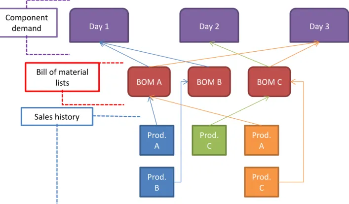
Since data of component picks is not readily available from AQ Electric Suzhou’s ERP system it was decided that component demand would have to be constructed by combining a sales list for all products with the relevant bill of material lists for these products. For each component a list of product(s) that the component is included in (as specified by the BOMs) is created. The list of product(s) is referenced to the sales history and for each day the in the sales history where the

product(s) has been sold the quantity of the component required for the assembly of that product(s) (as specified by the BOMs) is added to the demand of the component for that day. This process is

repeated for each component.

By deriving the component demand in this manner one avoids issues of incorrectly documented picking due to human error in the ERP-employee interface. At the same time, one loses visibility of factors such as component breakage and missing components. These issues were however found to be negligible according to AQ Electric Suzhou and the method can as such be considered viable.

The resulting measurement is the demand for each component per day over the period covered by the sales history (and forecast)4, which is then divided into weeks, with a corresponding estimated mean and standard deviation

4_{The period typically extends over one year.}

Prod.

A

Prod.

C

Prod.

A

Prod.

B

Prod.

C

BOM A

BOM B

BOM C

Day 1

Day 2

Day 3

Sales history

Bill of material

lists

Component

demand

(17)

16

6 Analyze

The third step was to analyze the data, determine distributions of demand for components and materials that were suitable, and derive distributions of inventory levels. This was simultaneously developed and integrated with the program.

Two methods for representing the demand for a certain component over a period of time have been considered; an empirical demand table with estimated frequencies and standard probability

distributions with estimated parameters. The empirical table consists of a set of demand sizes where the probability of each demand size would correspond to the relative frequency of said demand size, solely based on what has occurred previously. A probability distribution with estimated parameters attempts to match the distribution of demand with an estimated mean and standard deviation but allows for demand sizes that have not previously occurred.

There are two main issues with empirical demand tables for this application:

 The possibilities for future demand are rigid, if a demand size has not occurred previously then it cannot occur based on an empirical demand table even though it may be actually be possible.

 The mathematical methods are limited, analytical models are based on probability

distributions which mean that simulation models may have to be used. These models would be complex and difficult to standardize for individual components. In addition, it would not be feasible to perform a simulation for each component when there are thousands of components to consider.

As such estimated probability distributions were deemed to be the most suitable alternative.

Several components are used in high quantities in their respective products. At the same time most product types are seldom sold in higher quantities than 3-5 per week. This leads to a situation where the demands for many components can only assume a relatively small number of values. This ‘lumpiness’ in demand is difficult to capture with many probability distributions. One of the more intuitive ways to capture this lumpiness is through the compound Poisson distribution. If the orders arrive according to a Poisson process one can use an empirical compounding distribution (based on the size and frequency of individual orders) to derive the demand distribution.

If the demand is smoother one can consider the usage of the negative binomial distribution. If the customer can demand non-integer quantities a normal distribution may be more appropriate. Since the negative binomial distribution is a compound Poisson distribution with a logarithmic compounding distribution the variance must be greater than the mean as has been previously shown. The normal distribution has no such limitation on the relationship between mean and variance. However, the greater the variance the greater is the probability of negative demand. A similar relationship between inventory position, inventory level and lead time as for the compound Poisson case can be derived for the normal distribution (Axsäter, 2006), but since it rests upon an approximation that the probability for negative demand is insignificant attempts to represent stochastic demand with relatively high

(18)

17

variance in comparison to mean can yield poor results. The negative binomial distribution however, due to consisting of a Poisson process with a strictly positive compounding distribution, has no probability of negative demand.

Figure 5: Example of a negative binomial distribution (dots) and a normal distribution (curve), both with a mean of 5 and a variance of 10.

There are several other probability distributions that could be used to represent lead time demand, though these were found to be the most appropriate. The compound Poisson distribution lends itself well to describe the lead time demand in this case since the customer demand sizes are generally discrete and a limited amount of customer arrivals during the lead time. The normal distribution could be used in the cases when high numbers of customers arrive demanding small quantities due to the central limit theorem (as long as the variance is sufficiently small in comparison to the mean).

A compound Poisson distribution is similar to a Poisson distribution in that arrivals occur according to a Poisson process with a certain intensity λ. For a compound Poisson distribution however, the

cumulative stochastic variable is the sum of all arrivals multiplied by their respective compounding factor. This compounding factor follows a stochastic probability distribution and its range is usually taken to consist of integers (1, 2, 3,….) for simplicity’s sake.

For a Poisson process the probability of x arrivals during time t equals the following expression:

(19)

18

The expression for the stochastic variable YP(X=j) after t units of time following a compound Poisson distribution is similar to the above expression with the difference that the compounding factor must be taken into consideration. To that end let denote the probability that a stochastic variable from the compounding distribution is equal to j. Similarly, let denote the probability that the sum of k stochastic variables following an identical compounding distribution (k arrivals) yield a sum of j. Since

And

An expression for can be achieved through convolution:

∑

It then follows that

(2)

∑

Let

During one unit of time (t = 1). We then have:

With equality if Y follows a Poisson distribution, i.e. . (Axsäter, 2006). This imposes an explicit limitation on the relationship between the variance and the mean of j.

In the case that the lead time demand follows a negative binomial distribution it can be shown(Axsäter 2006) that the following is true for the lead time demand , .

(3)

k = 0,1,2,3…

Where Γ is the gamma function and r and p are parameter estimated from the mean and standard deviation of the lead time demand ( and respectively) in the following manner:

(20)

19

Let D(L) denote the demand during the lead time which follows a compound Poisson distribution. The following expression can then be used in order to determine the stationary probabilities for the

inventory levels for a continuous review (R,Q) inventory system (Axsäter, 2006):

(4)

∑

After deriving the component demand per day as per the method explained previously several goodness-of-fit tests were performed on all components’ historical data, on a level of significance of 5%.

The first test was for determining whether customer arrivals follow an exponential distribution with a mean estimated from aforementioned historical data. The test series was derived by finding the time between customer arrivals (in workdays): Let be the date at which customer i arrives and be the inter-arrival time for customer i and a total of n customer arrivals. and are then calculated from the following expressions:

∑

The second test was for determining if the demand per week followed a normal distribution with a mean and standard deviation estimated from the historical data. Demand per week was chosen as a basis for the test instead of lead time due to the lead time occasionally being long in comparison to the period of the historical data (e.g. 90 work days of lead time and a year of historical data available). The mean and standard deviation was the estimated through the following expressions:

Let be the demand during week i, with a total of n weeks.

(21)

20

√∑

In order to gauge how the weekly demand for the components could be represented Pearson’s goodness-of-fit test was used (for more information see Blom, Enger, Englund,Grandell, Holst). The first test showed that about half of the components’ customer arrivals could be described as following exponential distributions with estimated means. The second test however failed all the components. Since the vast majority of the components had a variance-to –mean ratio yielding relatively high probabilities for negative demand 5 it was decided that the normal distribution would have to be discarded.

Since the first test showed that a significant number of components’ customer arrivals could be

considered to follow exponential distributions it was decided that Poisson processes would be the most appropriate distributions for representing lead time demand. Since standard deviation for customer arrivals was higher than the mean in several cases (for the exponential distribution mean and standard deviation are equal) the overall variance in demand for these components will be underestimated or overestimated should the opposite be the case. This was considered an acceptable drawback since the Poisson process in conjunction with a compound distribution represented the logic of the order arrival and customer demand size well. Still, if the difference between measured standard deviation in lead time demand and the standard deviation of lead time demand according to a compound Poisson process with empirical compounding distribution be high6 a negative binomial distribution with correct mean and standard deviation will be chosen instead. In addition, should the overestimated variance prove too much of a burden the service level could be lowered to compensate.

Using a Poisson process with an empirical compounding distribution can however be computationally taxing due to the amount of combinatorial calculations needed when convoluting. Since more possible combinations also lead to a smoother demand distribution the negative binomial distribution is not only faster but also a suitable approximation in the aforementioned case.

As such it was decided that the negative binomial distribution was a suitable replacement in those cases.

Thus, it was decided that the program should represent the demand for the components with either  A Poisson process with estimated arrival times

 A compound Poisson process with an empirical compounding distribution and estimated arrival times

 A negative binomial distribution with estimated mean and variance

5_{1% chance or greater, which would contradict the approximation of continuously distributed inventory} positions.

(22)

21

7 Improve

The fourth step refers to the implementation of the program and the utilization of the program to identify and prioritize possible improvements that can be applied to the management of inventory at AQ Electric Suzhou. This is accomplished through the development of a system that is structured and simple to use. It mathematically models the metrics that serve as the targets in their operations, such as inventory levels, inventory value and turn rates, and optimizes reorder points based on these targets.

The average stock on hand, is obtained from the following expression:

(5)

∑

For a particular component the average tied up capital, in inventory is taken as the average level of stock on hand multiplied with the standard price, p, of the component:

(6)

∑

Let be the mean weekly demand. The number of times per year that the average inventory is turned is then calculated as the following:

(7)

⁄

1. Determine a lead time demand distribution

a. Use either (2) or (3) depending on choice of distribution, see appendix C 2. Find the smallest R that satisfies the service level constraint

a. Use the minimum order quantity as Q b. Use (1) as target function

c. Use a half-interval search to find an optimal R, see appendix C

3. Confirm that the found R fulfills the requirements of maximum inventory and turn rate a. Calculate a maximum allowed R by comparing the R from 2.c with the turn rate from

(7) and the maximum allowed inventory level7

7

The maximum allowed inventory level is a target parameter from the Excel file set for each component. The maximum R from this constraint is given by subtracting Q from the desired value

(23)

22

b. If the maximum R is lower than the R given in 2.c perform another half interval search using (7) as a target function. This alternative R will complement the R from 2.c and serve as a basis for comparison.

4. Print data

A typical approach to finding an optimal pair of Q and R is to begin with a fixed Q determined by economic order quantity or some form of restriction such as minimum order quantity. After an

appropriate Q has been found R is later optimized in regards to the objective function. Although a joint optimization of Q and R is also possible it is generally sufficient to proceed with the method above (Axsäter, 2006) During a discussion with AQ Electric Suzhou it was found that the order cost was bordering to insignificantly small and that there were no readily available figures for holding costs. As such it was concluded that finding a suitable Q by applying the economic order quantity would not yield accurate or particularly trustworthy results. Since the results from the economic order quantity formula would still be subject to the minimum order quantities it was then decided that the minimum order quantity would be used as Q.

The next step is to determine the R that fulfills either a target service level or a maximum average stock on hand. The service level function has a lower bound in , which will yield a service level of 0, but in theory has no upper bound since the theoretical distributions also lack an upper bound. This is handled in practicality by setting an artificial boundary on the demand distribution functions at a sufficiently high value, in this case the limit was set at the value which yields a cumulative probability of 0.999. This speeds up calculations significantly since the vectors do not have to be infinite. Now that the demand distribution has an upper bound the service level also has an upper bound in .

An exhaustive search of all values for R in the interval [-Q, Max[D(L)] ] is however far too

computationally taxing to perform for several hundred components whose spans can well contain up to several thousands of values. As such, a half-interval search is employed to find the optimal R by using fewer calculations since the algorithm only has to calculate current lower bound, middle element and upper bound for a limited number of iterations. A prerequisite for this algorithm to be viable is that all the elements in the array to be searched have been sorted from lowest to highest. Due to the Poisson process with full backordering assumption a higher R will always yield a higher service, the turn rate will similarly strictly decrease with R. As such the algorithm can be used without risk of yielding incorrect results.

The calculations were performed by the program on the components used in the electrical cabinets provided to Tetra Pak in order to determine the benefits that can be attained from using it. Since AQ Electric Suzhou focuses on service levels and turn rates of 98% and 16 times a year respectively these were the target parameters that were set for optimization.

The components that were chosen for this comparison were those that were used for AQ Electric Suzhou’s highest volume product families, since these components have the most reliable historical data available and the results are therefore more representative.

(24)

23

Average Inventory Value Average Turn Rate Average Service Level Min Service Level Max Service Level

Target: 16 turns per year 457 976 18.18 0,609 0 0.996

Target: 98% on time delivery 1 056 201 7.82 0,984 0.9800 0.999

Historical inventory data 2 185 024 - - - -

Table 1: Comparison of historical data with the results of the program

Although it is obvious that there exists a trade-off between service levels and turn rates the purpose was to investigate what the impact would be on average inventory values, service levels and turn rates so that AQ can make an informed decision regarding their targets. The average inventory value was calculated by the program by multiplying the average positive inventory level by the standard price of the component . Similar calculations were performed for the historical data but the average positive inventory was calculated by considering the negative inventory levels to be 0.

∑

The average turn rate is the turn rate of the entire inventory which is calculated in the following manner:

Let be the expected turn rate for component i.

∑ _∑

The result was that achieving the target of 16 turns per year for each component results in a significant decrease in service levels which is inconsistent with AQ Electric Suzhou’s target of an on time

delivery of 98% for their products since it can’t be higher than the highest service level of an

individual component present in the assembly of the product. It’s worth mentioning that the decrease in average inventory is off-set by a decrease in average service level at a rate of 598 225 CNY to 0.375 in this case. Finally, it is clear that the program can result in significant savings while

maintaining the target for on time delivery. If the target service level for each component is set to 98% it results in a reduction of the average inventory value by 1 128 823 CNY and the difference remains high even when optimizing for high target service levels. This confirms the suspicion that AQ Electric Suzhou simply has too much of what they don’t need and too little of what they do need. In addition, it would seem that a more suitable approach to increasing the average turn rate would be to negotiate with suppliers in an attempt to reduce the minimum order quantities for components. In many cases there are large quantities for components with low demand resulting in turn rates that are low. Reducing the minimum order quantities would result in an increase in turn rates without decreasing the service levels, for example.

(25)

24

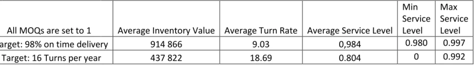
All MOQs are set to 1 Average Inventory Value Average Turn Rate Average Service Level Min Service Level Max Service Level

Target: 98% on time delivery 914 866 9.03 0,984 0.980 0.997

Target: 16 Turns per year 437 822 18.69 0.804 0 0.992

Table 2: Using a minimum order quantity equal to 1 for all components

The results indicate that the goals of 98% on time delivery and 16 turns per year are difficult to achieve simultaneously. The average service level does not provide a suitable approximation for on time delivery since the on time delivery will be bottlenecked by those components with a low service level. Indeed, certain components have a service level of 0 when optimizing for 16 turns per year since the only way to achieve or exceed this target is to have nothing in inventory at all.

In order to achieve greater results one must instead turn to improving other parameters such as lead time, minimum order quantity or takt change time. The service levels for individual components do not necessarily have to be identical either. Low cost components can for example have higher service levels than the high expense components which could lead to higher on time delivery without the total cost increasing significantly. It is however not feasible to achieve 98% on time delivery and an average turn rate of 16 with the above method since the on time delivery is approximately the minimum of the individual components’ service levels as discussed in the Finding suitable

measurements for service levels chapter.

The program should prove to be valuable for AQ Electric Suzhou and its role as an analytical tool proved to be valuable during our stay in Suzhou where the program identified multiple lead times and minimum order quantities that AQ Electric Suzhou deemed to be unacceptable.

In general the process of implementing inventory control is not as linear in practice as it would seem in theory. The initial approach was to find perfect probability distributions for the demand of each component by using the chi-squared method. This proved futile as there were many components and in certain cases the data would seem to follow a distribution well when plotted but would not be

approved by the chi-squared method. Since the purpose was not to find distributions that would satisfy the chi-squared method but distributions that captured the critical qualities of the demand of the component (such as mean, variance, discrete and/or if it was lumpy8) that method was abandoned in favor of a simplified and standardized method based on the empirical compound Poisson distribution. This method worked well initially but there were issues in regard to computational complexity which we were inexperienced with as it was never an issue that occurred during the courses in inventory control. The solution was that in certain cases we utilized a negative binomial distribution instead which alleviated the computational complexity in those cases but was not as suitable to the original demand distribution as the empirical compound Poisson distribution. Another issue that was present through the project was the quality, quantity and availability of data. In certain cases we had data that was conflicting, incomplete and inconsistent while being of different formats. The format issues was a particularly difficult problem as it is difficult developing code that performs calculations and

commands automatically when the format differs.

(26)

25

8 Control

The fifth step is a continuous process that is applied in parallel to the previous steps. Issues may be identified in later steps based on applications, developments and decisions made in earlier steps. The application of control means that the methodology becomes iterative and that the system is holistic. Comparisons made between the theoretical values and empirical values in addition to issues that were identified when running the program, such as accuracy and performance, should be utilized to improve the program further. There is usually a trade-off between accuracy and performance and it is

important to ensure that increases in computational precision are not negated by increases in

computational complexity. Since the number of components and materials was large decisions had to be made regarding the use of standardized solutions as opposed to custom solutions. Specifically in regard to the complexity that such a decision would introduce since standardized solutions are generally simpler to implement, review and monitor.

An important distinction is that many possible improvements cannot be attained and/or verified until the system is implemented in the operations of AQ Electric. As such, the process of reviewing and monitoring should not just be applied during the course of the project but also during the utilization of the program by AQ Electric Suzhou in the future. It is vital that results from the program are

continuously examined and evaluated by them. Especially since some assumptions that were made during development, such as all components sharing the same takt change time, may be irrelevant or inaccurate in the future.

On our part there is an ongoing process of identifying and eliminating issues that occur during the use of the program. Due to the variability of the data that can be imported, in both quantity and quality, it is difficult to prevent all possible sources of error that may occur when using the program. In

particular, issues that occur due to the user such as the usage of inaccurate, incomplete and/or incorrect input can be difficult to prevent. There is also the issue that it is difficult to determine the absence of errors which is similar to proving a negative where the absence of evidence is not evidence of absence. On AQ Electric Suzhou’s part there should be an ongoing process of reviewing their use of target service levels, target turn rates and the effect of maximum inventories on their operations. The accuracy of input data such as lead times and minimum order quantities has a significant effect on the optimality of the parameters that are calculated by the program. It is important that the output data provided by the program is analyzed and discussed within AQ Electric Suzhou. Partially because it facilitates the process of identifying and eliminating errors that may occur but also because it can serve as a basis for improvement when negotiating contracts with customers and/or suppliers.

9 Implementation

Implementation of inventory control is more difficult in practice than in theory, as courses and

literature would indicate. Especially when the implementation is for many different components and it needs to be able to be run for sets of components and data that is different from what one currently has access to. Normal procedure may involve performing modelling and calculations for a set of

components and data once for a specific set of components and data during a specified period of time. This is comparatively simple since if the modelling and calculations are correct for that set of

components and data then that’s all that is necessary. In this application there was also a need to ensure that the program was adaptable and flexible to the degree that it could perform calculations for components and data that one has not had access to previously. This can be quite deceiving and difficult since calculations may work perfectly for a previous set of components and data but suddenly

(27)

26

when there is an update there may be complications. An example could be a component that yields a ratio between its mean and variance in such a way that calculations become too time consuming. Such problems are difficult to consider since they are reliant on experience to identify and difficult to predict.

Previous applications of inventory control during our studies were usually on a single component were computational complexity was not an issue. The calculations in this implementation had to be

performed on thousands of components which meant that computation complexity became a real and tangible issue. Many adaptations and decisions had to be made in order to reduce computational complexity and reduce the number of iterations that had to be performed. An example of this is the half-interval search. Originally when the program was being developed for a sample of components all searches were exhaustive searches were the reorder point would start at the lower bound and increased by increments of one up to the upper bound until the target service level was achieved. This became far too time consuming when the interval between the lower bound and the upper bound could consist of thousands of integers and there were thousands of components. An adaptation had to be made on the basis of the target function being either strictly decreasing (turn rate) or increasing (order line fill rate). Another problem that frequently occurred was that the format of the data being exported from Monitor would vary. Either due to different people providing it from a different source(s) and/or in a different format(s) or because the format itself would vary slightly when exporting it (such as variations in indentation, columns and rows). Adaptations had to be made in the program to consider and adapt to these variations in format that could occur. Although such adaptations only prevent that specific issue from occurring again.

10 Conclusion

On the whole the results indicate that AQ Electric Suzhou will be hard pressed to achieve both targets of on time delivery and target turn rate at the same time. On the other hand, the results also show that the amount of tied up capital can be significantly reduced from the current setup even with a constraint of 98% on time delivery. A cause of this can be that no structured review of the inventory parameters and demand data has previously been carried out, meaning that certain components have far too high inventory levels and other components far too low and thus bottleneck the on time delivery while overall inventory levels are high. As such, even if the results from the program would prove too optimistic one can still expect to see significant improvements from implementing the results.

(28)

27

References

DMAIC, http://www.isixsigma.com/dictionary/dmaic/

J. Song, On the Order Fill Rate in a Multi-Item, Base-Stock Inventory System, Operations

Research Volume: 46 Issue: 6 (1998-11-01) p. 831-845. ISSN: 0030-364X

G. Blom, J. Enger, G. Englund, J.Grandell, L. Holst, Sannolikhetsteori och statistikteori med

tillämpningar, Studentlitteratur AB

K.M.R. Hoen; R. Güllü; G.J. van Houtum; I.M.H. Vliegen , A simple and accurate approximation for

the order fill rates in lost-sales Assemble-to-Order systems, In Leading Edge of Inventory

Research, International Journal of Production Economics..

Axsäter, Sven (2006), Inventory Control, Springer Science+Business Media, LLC Silver, E. A., D. F. Pyke, and R. Peterson. 1998, Inventory Management and

(29)

28

Appendix

A. Program Presentation

This section will present the program along with its features. The purpose behind the program was to provide AQ Electric Suzhou with a standardized method of determining the reorder points for their components in order to maintain their target service levels while reducing the amount of inventory being held. It is also meant to serve as an analytical tool by attaining and aggregating the vast data found in various sections of their ERP-system and presenting it in a clear and concise manner and simplifying the process of identifying excessive lead times and/or minimum order quantities for example.

The choice of VBA was based on previous familiarity with it, it is used in Microsoft Excel and thus available without AQ Electric Suzhou needing to purchase a separate license. In addition, it is simpler to extract and format data from Monitor since the exports are commonly in the Excel- or Text-format which are suitable for being imported into Excel.

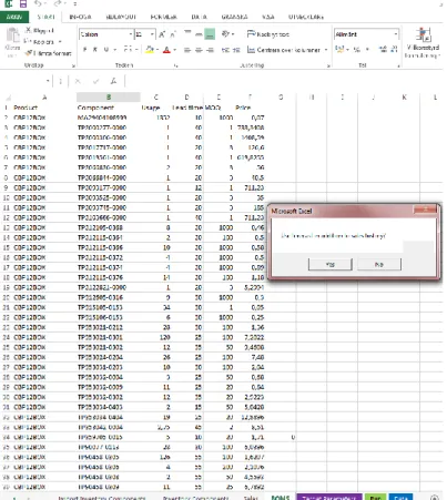
The program consists of an Excel-file with a set of specified sheets and extensive code. It requires that a set of files have been placed in indexed folders located on the main server at AQ Electric Suzhou. The indexed folders are BOMS, Components, Forecasts and Sales and the files are obtained by exporting the data in the specified format from the ERP-system Monitor. In BOMS the user places a text file for each product that contains the bill of components and in Components the user places an Excel-file containing the corresponding data for those components/materials (average lead times, minimum order quantities and suppliers). The remaining files are Excel-files for forecasts (which are optional) and sales history (which are obligatory) detailing the date and quantity for each product in an order for a period of time (generally a year). The import process will prompt the user whether to use forecast in addition to sales history.

(30)

29

Figure 6: The prompt whether to use forecast in addition to sales history

The program needs to import the data from the files that were prepared. This is done on the “Run”-sheet by pressing the “Import Data”-button which causes Excel to import the data from the files in the indexed folders located on the main server.

(31)

30 Figure 7: The "Run"-sheet

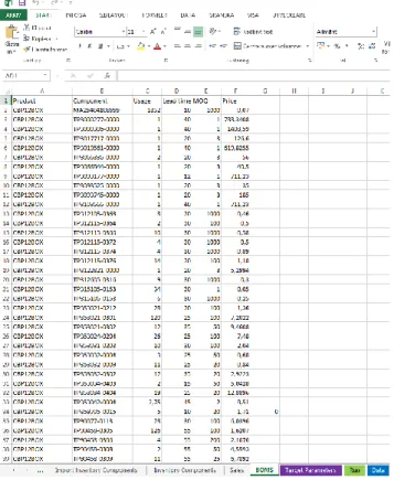
It then aggregates and structures the data so that the format is suitable for the calculations that will be performed by the program and the result is provided in the sheets “Inventory Components”, “Sales” and “BOMS” which can be seen below.

(32)

31 Figure 8: The resulting "BOMS"-sheet after import

(33)

32

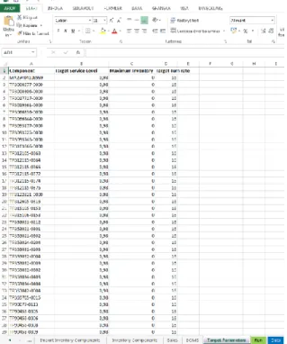
The sheet “Target parameters” allows the user to specify the target service level, maximum allowed inventory and target turn rate for optimization for each component. If no target parameters are

provided then the program will set them to a default of 98% target service level, no maximum allowed inventory and no target turn rate. The maximum inventory is mainly used when AQ Electric Suzhou has a stock agreement specifying the maximum amount of inventory for certain components that their customer will compensate them for if it becomes obsolete due to changes in design or sourcing for example.

Figure 10: The "Target parameters"-sheet

If the data has been imported then the program can perform the calculations by pressing the “Calculate parameters”-button on the “Run”-sheet. If desired the program can perform the calculations for a set of components specified in a list on the “Run”-sheet by selecting “Yes” when prompted to “Calculate parameters for specified components only?”.

(34)

33 Figure 11: The prompt to calculate for specified components

After the program has performed the calculations the data is presented in the “Data”-sheet. It contains the order quantity, reorder point, service level as well as the expected inventory level, value and turn rate for each component. If the target parameters maximum allowed inventory and target turn rate were set previously then the maximum allowed reorder point and the corresponding expected inventory level, value and turn rate will be provided as well.

(35)

34 Figure 32: The output of the program

(36)

35

B. Import

Creates a list containing the number of products demanded at a particular date and the products’ component usage (i.e. how many components each product needs at a certain date). These dates are later grouped into weeks. The mean and standard deviation ( ) of the demand per week is then calculated according to:

∑

Where n is the number of weeks and i is the index for the total component demand week i. The lead time demand mean (µ) and standard deviation (σ) is then calculated:

√

Where L is the lead time for the component minus the takt change time, in working weeks.

C. Optimization

An empirical compounding distribution is calculated according to

∑

Where the demand sizes have been scaled with the greatest common denominator9 Where is the number of component demand sizes of j units.

Let be the expected standard deviation from a compound Poisson process with an empirical compounding distribution and an arrival intensity of λ. The following expression then holds true (Axsäter 2006):

√ ∑

Where the λ is taken as the total amount of ordered products divided by the time period covered by the sales history.

9_{If, for example, all demand sizes have been 10,15 or 20 they are then converted to 2,3, and 4 respectively. This} speeds up calculations but is also necessary in order for the inventory position to be equally distributed over R+1 To R+Q (Axsäter 2006).

(37)

36

Based on the data previously synthesized as per above, the following rule decides what probability distribution is to be used:

Let be defined as ∑

I.e. there is a 99.9% chance of or fewer demanded units of a product during the lead time minus the takt change time.

If the ratio is greater than 1.25 or smaller than 0.75, Max j * is less than 15000 and

1 :

Use the negative binomial distribution for modeling the lead time demand. Else, use a compound Poisson distribution using and .

The first ratio is used to prefer the negative Binomial distribution if the compound Poisson with empirical compounding distribution would yield a significantly different variance than what has been measured. The second constraint is based on how computationally taxing it would be to compute lead time distribution and optimization for the compound Poisson distribution, where 15000 is a limit that has empirically proven to yield in acceptable results . The final constraint is necessary since the variance of the negative Binomial distribution is strictly greater than 1.

After a lead time demand distribution has been chosen an optimal reorder point is found by using a half-interval search. If this reorder point will yield a higher maximum inventory or lower turnover than specified in the “Target Parameters” worksheet an alternative R is also found, also using a

half-interval search.

Let be the upper bound and be the lower bound of a set of integers : S = { . Let be a one dimensional function and

Let be the target value to be found and

The algorithm for optimizing for a certain T is the following: A. Let

, rounded up to an integer. B. If let , go to A. C. If let , go to A.

D. If , end the algorithm using as return value. E. If , end the algorithm using as return value.

Step E comes into effect when there is no that satisfies step D. This means that any integer in the Set S will have a functional value greater than or lesser than T and . In this case one wants to find the smallest integer that exceeds or is equal to T, as such is chosen as return value. If

is the case one simply reverses the inequalities in step B and C.

Inventory Control at AQ Electric Suzhou