FOCUSING OF UWB RADAR SIGNALS USING TIME REVERSAL

(1)

FACULTY OF ENGINEERING AND SUSTAINABLE DEVELOPMENT

FOCUSING OF UWB RADAR SIGNALS USING

TIME REVERSAL

Faheem Ahmad & Pramod Kakkerla

September 2013

Master’s Thesis in Electronics/Telecommunication

Master’s Program in Electronics/Telecommunications

Examiner: Niclas Björsell

(2)

(3)

Preface

We would like to thank both teaching institutions, University of Gävle and Radarbolaget. Without the help of these remarkable establishments, it would have been impossible for us to carry out this research. We would like to thank our supervisor Mr. Daniel Andersson who was always available for meetings. He really led us the whole path we have been through to the completion. We are very grateful to Patrik Ottoson who accepted us for this research and guided us in writing this report. We would also like to thank the whole staff at University of Gävle who steered us whenever we were held.

Finally we would like to thank our parents, family, and friends who were always benevolent, compassionate and kept pushing us in the completion of this research.

(4)

Abstract

Focusing techniques and detection of targets is usually associated to defense and military use. However in recent past things have moved ahead. Now target detection using UWB radars is being done in many industries and corporations. Radarbolaget AB is one of them; one of their projects uses UWB radars to detect steel strips inside a furnace.

This research solves a potential problem of detecting middle steel strip out of total three strip edges which can be seen by radar placed on the front. For better understanding of the reader, existing system and introductory UWB radar principles are discussed. As there can be many solutions to focusing of targets here (steel strip edge detection). Available focusing techniques have been discussed in detail along with the possible physical and simulation setups. Later in the document, detection methods have been proposed. UWB time reversed signal detection is a fairly new method and a very limited research has been done so far. PRBS sequence has been focused on in detection mechanism.

Results section show that the pulse of the PRBS works better and produces more promising results rather than a repetitive signal. Time reversal methods for locating the target have been used to find the approximate location of the target. Manual distance calculations from target to the transmitter and receiver have been done. Comparison of actual distance from target to the transmitter is compared with simulation results. Different model simulation setups and their results have proved that using UWB Time reversed signals; a still or moving target can be detected with centimeter window precision.

(5)

Acronyms

2D Two Dimensional

AAS Adaptive Antenna System

DTV Digital Television

FCC Federal Communications Commission

FFT Fast Fourier Transform

GPR Ground Penetrating Radar

IIR Infinite Impulse Response LFSR Linear-feedback Shift Register MANs Metropolitan Area Networks

MATLAB Matrix Lab

MIMO Multiple Input Multiple Output MISO Multiple Input Single Output

PN Pseudorandom

PRBS Pseudo-Random Binary Sequence PRF Pulse Repetition Frequency

RADAR Radio Detection and Ranging

RX Receiver

SAR Synthetic Aperture Radar

SD Spatial Diversity

SIMO Single Input Multiple Outputs SISO Single Input Single Output SLAR Side-Looking Airborne Radar SM Spatial Multiplexing

SSRG Simple Shift Registers

(8)

UWB Ultra Wideband

WLANs Wireless Local Area Networks WPR Wall Penetrating Radar

(9)

1 Introduction

1.1 Background

Traditional narrow band frequency equipment has many advantages and yet many flaws. Narrow band signals use a limited bandwidth and limit the information capability of radio systems. There are many cases where huge chunks of information need to be processed and narrow band systems are not the solution. However, Ultra-wideband (UWB) systems are the solution for providing a higher bandwidth.

Detection and measurement accuracy is one of the major advantages of UWB radars thanks to more information and more robust signals. Smaller pulses can be transmitted in fractions of seconds and reflected signals can be used to monitor targets. Variations in signal generation are huge and can be fully controlled by changing the signal wave forms. Target accuracy can be increased to millimeter or sub-millimeters ranges. Detection of shape and size of objects is possible with the received signals because the received signal carries huge information.

UWB radars are also very common for detection of objects behind walls and targets in non-line of sight conditions. High frequency radar pulses can penetrate many of the common dielectric materials such as in ground, rocks, concrete walls, plastic, water, wood, snow and ice, However the reflected signals are highly attenuated and special UWB receivers are required for detection.

Based on the property of penetration there are thousands of applications today where UWB radars are used and this thesis describes one of them. Received signals with multi input multi output (MIMO) antenna systems have shown that reflections from various objects can be utilized in our favor. Multipath propagation can be used as an advantage by time reversal for better resolution of received signals. Surely, multipath can bring lot of clutter into measurements. Using time reversed signals and transmitting them again towards the target can improve focusing of targets in a great manner.

Time reversed signals go through the same diffraction, refraction and attenuation as they go through in forward direction. Initial source is then surrounded by higher energy levels. Time reversal which is a signal processing technique can be done to obtain a focused area where targets might be.

(10)

1.2 Existing System

We have done this thesis with Radarbolaget, a company which is providing solutions to complex radar measurements. Major projects of the company include edge detection and measurements of steel and metal sheets with the help of radar sensors outside a furnace wall.

As the temperature inside a furnace is more than 1000 C, it is necessary to do measurements from outside of the wall. UWB wall penetrating radar (WPR) is the only solution thanks to the robustness of its radar signals. Steel sheets and plates are being treated inside the furnace and there are rollers which move them. In order to keep the alignment between rollers and plates, it is needed to determine the position of the plate and move it to the middle of the furnace. Using radar outside the furnace walls, it is possible to monitor the position of the plates. Figure 1.1 explains how the plates are placed on the rollers inside the furnace.

Figure 1.1: Model process of metal sheets and plates inside furnace

1.3 Problem Statement

In some places where a system for strip guiding will be installed, there will be parallel strips inside the furnaces. This could be a problem since the radar system will also “see” the edges of the parallel strips and maybe treat them as the closest targets. Figure 1.1 shows an installation with parallel strips, the black boxes are the radar units. It is vital that the radar only tracks the movements of the strip edge in front of the radar.

The target signal of the steel strip edge is estimated from the difference between a reference measurement, where there is no strip inside or a pilot strip, and a target measurement, where there are

(11)

strips in place. If the decision model only detects changes, some sort of target tracking has to be implemented that distinguishes the strips from each other. The problem is when there are three similar targets and we need to focus on the middle one. If it is possible to focus and keep track of the middle plate then it is very easy to see if the metal sheet is going off the roller or not.

(12)

2 Ultra-Wideband Radar Systems

2.1 Background

The word “RADAR” is an abbreviation and stands for “Radio Detection and Ranging” (and it is also a palindrome). Radar systems were developed for surveillance and target detection purposes in preparations to World War II. The term ultra-wideband (UWB) was widely accepted after 1990’s. A UWB signal is defined as a signal whose bandwidth is more than 25% of its center frequency [1].

There are many ways in which radar transmitter and receiver can be placed. Basic three types are: Bi-static, Mono-static and Quasi-Monostatic. Bi-static radars have their transmitter and receiver at different locations from the target. Mono-static radars have the transceiver (transmitter and receiver) on one location as seen from the target. Quasi-Monostatic radars have their transmitter and receiver antenna almost at the same location but still there is a small gap between transmitter and receiver. We have used Quasi-Monostatic UWB radar in our thesis. Typically radars operate from 3 MHz to 300 GHz depending upon the application [2].

Figure 2.1: Basic Principle of Radar

Where, is distance between RX and target, is the distance between TX and target and θ is the angle of reflection.

Figure 2.1 explains the basic principle of radar. The transmitting antenna is the TX and receiving antenna is the RX. The transmitter sends a pulse to the target and reflected pulse is received at the receiver. It is very important to consider the electromagnetic spectrum or set of frequencies used by the radar system. The spectrum varies from high frequencies up to infrared range. Figure 2.2 explains the electromagnetic spectrum [2], and typical frequencies at which radars operate.

(13)

Figure 2.2: Electromagnetic spectrum marked with typical radars frequencies

2.2 Ultra-Wideband Radar System

Most of the radio systems use a band of limited spectrum and a narrow set of frequencies. These frequencies are then modulated with the carrier wave and transmitted through the channel. The main reason of doing this is that, it is very easy to implement frequency selection based on limited frequency band. FCC has allocated 3.1-10.6 GHz frequency spectrum for UWB communications [3].

A majority of the radio systems have lower frequencies than their carrier signal. These narrow band systems limit the information capability of radio systems, because the amount of transmitted information is directly proportional to the frequency band. To increase the information capacity, is also needed to increase the frequency band. However, we can also use modern equipment and send information in shorter time. But this method has some limitations so, wider bandwidth is very important for modern radio systems.

Robert Arno Scholtz a renowned professor of electrical engineering at the University of Southern California gave a concept of wideband wireless technology [3]. Frequency spectrum in ultra-wide band usually considered very high. In microwave ranges it can make our signals ultra-ultra-wide by using the higher bandwidth. Most ultra-wideband radars use a bandwidth of more than 25% of the center frequency. A bandwidth of 800 MHz – 1 GHz is used with a center frequency of 2 GHz.

(14)

UWB radar systems can be built for many applications, currently they are being used for medical, military, construction, weather, and traffic purposes. UWB radars use a large number of short pulses in fractions of seconds. Signals used in this thesis are transmitted at a rate of 4 gigabits per second which means a pulse every 250 picoseconds.

Short pulses are very useful for detection of the target. For example, the resolution to resolve a 12 mm target, a pulse width of 40 picoseconds is needed. Transmission of very short duration pulses strict the power limitations and make the performance of UWB systems highly sensitive to timing errors. If we compare the energy density of UWB radar and conventional radar [4], we can see Equation 2.1 and 2.2. In equation 2.1, the energy density of isotropic antenna is given, while in Equation 2.2 energy density of directive UWB radar antenna is given.

2.1

2.2

Where,

energy density of isotropic antenna

= energy density of directive antenna

= energy of signal

R = distance between radar and target

G = gain transmitter antenna gain.

Equations 2.1 and 2.2 relate how the energy densities of conventional radar and UWB radars differ from each other. Directive antennas have higher gains in a specific direction. This phenomenon helps in detection of targets.

2.3 Waveform Selection

Waveform selection is a very important factor by which radars can be classified by their waveforms, and we can choose the waveform based upon the application in which it is being used. UWB waveforms have different characteristics compared to conventional waveforms mainly because of their wide-band selection. A wide-band range resolution can be determined by the following expression given in equation 2.3.

(15)

Where, = pulse width

= speed of light

B = bandwidth of a UWB signal

The expression explains that the improved range resolution is achieved because of higher bandwidth of UWB signals. As there is inverse proportion between pulse width and bandwidth, higher bandwidth will result in shorter pulses which speeds the process of pulse transmission. This is the main idea behind wideband systems because they are robust and more accurate than conventional narrow band systems.

Following is the breakdown of waveforms based on their class.

Radars

CW Pulsed

FMCW Non-Coherent Coherent

Low PRF Medium PRF High PRF

MTI Pulse Doppler

Figure 2.3: Classification of radar waveforms

Where,

MTI = Moving Target Indicator

PRF = Pulse Repetition Frequency

CW = Continuous Wave

FMCW = Frequency Modulated Carrier Wave

Coherent systems allow precise target detection. Phase of the carrier is already known which helps in demodulation of the signal. Pulses are generated in requirement to the application. Medium PRF can help to detect a target which is couple of feet in dimensions. However if the targets are small and edge detection is required high PRF is always a good choice. On the other hand non coherent and FMCW waveforms receiver carrier is not phase locked with the transmitter carrier.

(16)

2.4 Wall Penetrating Radar

WPR comes under the umbrella of ground penetrating radar (GPR). Both WPR and GPR are considered as ultra-wideband radars. Today, ground penetrating radars have huge applications and used to detect underground mines, cavities, potential holes, monitoring of traffic, road construction and parking systems. Wall penetrating radars are popular in military surveillance and steel industry to detect metal sheets.

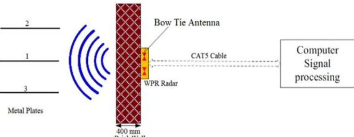
WPR outside a furnace wall with a thickness of approximately 400-500 mm is considered. A temperature of 1200 C inside the furnace is the actual reason WPR is used, but it is also important to protect electronics from iron dust and vapor.

A center frequency of 2 GHz is used, while bandwidth is kept between 800MHz - 1GHz. A very high sampling frequency is used for better resolution of the targets, i.e. 80 GHz. Waveform PRF is used as shown in Figure 2.3. Pulses are being transmitted at the rate of 4 gigabits/s. Radarbolaget’s software Radaradmin 1.2.10 is used to transmit and analyze signals.

Figure 2.4 WPR Implementation in real system

Figure 2.4 explains how wall penetrating radar is being used in our thesis. Signals are pushed to the radar processing unit using the Radaradmin software. The transmitted signals are received by the radar receiver. Received signal goes back to the computer for further processing in matlab.

(17)

3 Target Focusing Techniques

Radar concept is that it operates by radiating electromagnetic energy, and detects the echo from the target. We can find the range or distance based upon the time taken for radiated energy to travel to the object and back. The character of the echo signal provides information about the target. Moving target can also be traced by the radar and the radar can also estimate the target’s future location. Moving targets (like planes) can be separated from stationary targets (land or mountains) based upon the doppler effect caused by the shift in the frequency of the received signal, moving target magnitude is lesser than stationary echo signal.

Normal radar measurements provide distances, not directions. Therefore, it is troublesome to determine which target that is connected to which distance. Radar resolution can be done on the target to determine its location. If the radar resolution is good enough, it can forecast the nature of target i.e. size and shape. There are a number of possible techniques for focusing of targets using radars. Most of them are based on radar measurements performed from different positions. Possible methods are:

 Phased Antenna Array is a system in which multiple antennas work together to make an array. Relative phases of the respective signals are varied in such a way, that the effective radiation pattern of the array is reinforced in a desired direction and suppressed in undesired directions. Multiple measurements are used to compute geometric intersections. These intersections are drawn by using multiple signal propagation paths. Geometric intersections also provide data to produce pseudo images. Signal processing can be used to create pseudo images. All possible lengths from all antennas positions are reproduced in an aggregated image [5].

 Synthetic Aperture Radar (SAR) is using relative motion, between an antenna and its target region to obtain finer spatial resolution than possible with conventional beam-scanning.

 Time Reversal signal processing is a technique where the transmitted and received electromagnetic waves are reversed and transmitted again in a reversed order.

 Physical installation like Luneburg lenses, convex lenses, waveguides, and parabola dishes may focus the radar beam. Theoretically, it would be possible to construct refractory walls with focusing properties.

 Amplitude characteristics and its magnitude can be used if the targets are similar. This method should be handled with caution and only be used together with other methods, but in general the centered target has the highest amplitude and magnitude.

(18)

3.1 Phased Array Antenna

Antenna array define the group of multiple radiating elements coupled to a common source or load to produce a directive radiation pattern. Planar array is most common array method. In this array, horizontal and vertical elements are aligned in a linear way to form a plane [5].

Before radiation, array applies appropriate phase relationship to form wave front-flat. This kind of arrangements is not possible with lens and parabolic reflectors. Position of the beam is defined by the relative phase, this phenomena is called as phase array pattern. Due to this relationship, beam can be rotated or steered without antenna move. These properties of an array made them for scanning and tracking purposes ideally.

3.2 Multiple Antenna Solutions

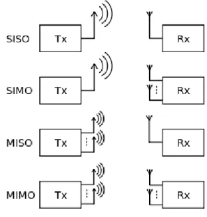
Multiple antenna technology is the most active research area to improve the robustness and performance of wireless links. There are several multiple antenna techniques Figure 3.1 among those Single Input Multiple Output (SIMO) has the widespread applications in digital television (DTV), wireless local area networks (WLANs), metropolitan area networks (MANs), shortwave radio operations and mobile communications. It provides the high speed data transmission and increase in the capacity of modern wireless communication fields from above feature SIMO enable the better wireless communication link for our test setup.

Figure 3.1: Different types of antenna setups

In order to focus on a target, multiple antennas can be used. The antennas is normally mounted outside a furnace and stacked into an array.

(19)

In this project following ideas using multiple antenna solutions have been considered.

 Simulation using multiple antenna solutions

 Multiple and simultaneous measurements in different antenna setups

 Correlations using multiple antenna systems

 Development of imaging methods using time reversal with multiple antenna systems

3.2.1 One Transmitter and One Receiver

Common radio frequency is shared between transmitter and receiver, Figure 3.2 shows typically structure of one transmitter and one receiver. There is no much complexity in the setup because of their common radio frequency sharing. This setup is usually used in personal Wireless technologies such as Wi-Fi and Television systems.

Figure 3.2: Setup for SISO

3.2.2 One Transmitter and Two Receivers

In this setup the user has freedom to choose the best signal from any of the receiver or grouping of two signals or aggregate, Figure 3.3represents the configuration of one transmitter and two receivers. This type of setup is used to improve the performance of the radio channels.

Figure 3.3: Setup for SIMO

However, there is a problem with quality of control in this phenomenon, because of high capacity and low error rate. A multipath fading effect has been used to maintain good quality of service. A transmitted signal is scattered on different objects and few of signals are reflected back to the receiver. These received signals are faded and distorted. This occurrence is called multipath fading. If different signals are used in frequency this may cause for the co-channel interference. In order to achieve

(20)

wireless transmission. These three parameters can be achieved when the radiation directing changes according to the traffic conditions in signal environment. In multiple antenna process, coding technology and signal processing method are playing a vital role. This technique is broadly divided in to three categories.

 Spatial Diversity (SD)

 Spatial Multiplexing (SM)

 Adaptive Antenna System (AAS)

3.3 Moving Antennas and SAR

Instead of having a fix array of antennas, it is possible to move a pair of antennas along a pre-defined route. The antenna pair can be mounted, for example in an industrial solution, on a linear unit. The airborne radar system called Carabas is using multiple measurements from different positions and the SAR technique to compute and portray the landscape in high resolution. SAR is commonly used in radar measurements from satellites. The technique is sometimes combined with SLAR.

In industrial solutions, very fast linear units or linear motors can be used as antenna transporters. The antenna position on a linear unit can be determined with the accuracy of ≤0.1 mm. The linear unit is fast, and up to 40-50 measurements can be performed in <1 second when the antennas are moved 800-1,000 mm. The major drawback is the measurement time from multiple positions, but the system could be a robust focusing device.

3.4 Time Reversal

Time reversal by impulse based UWB radar technology and combination of these two, has an ability to make many innovative radar applications in communication systems. A higher sampling rate is needed to sample the impulses and resend them. UWB radar can send very short (nano) pulses and each pulse has its own periodic nature which makes radar system resourceful for low-cost applications. The proposed time-reversal system is also tested with different trransceivers, free propagation is considered. The RF propagation channel suffers from time-varying impairments like multipath, interference, and noise. From past few years, a research work has been going on time-reversal technique for electromagnetic waves. Time time-reversal method enables high-resolution imaging in multipath surroundings.

Time reversal process is based upon two dimensional wave equations. A basic wave equation for is given in Equation 3.1 [6]. The signal is transmitted through the channel received by the receiver and retransmitted back on the same path it came from. By doing this, the wave is focused, and therefore it is not needed to solve the wave equation [6]. Time reversal has a huge scope and can be combined with UWB signals to focus on specific millimeter range targets.

(21)

3.1 Where, u = a scalar function

t = time variable

c = speed of light

= spatial laplacian operator

Time reversal method has attracted interests from engineers as well as physicists due to the potential focusing of waves in both space and time especially; time-reversal takes benefit of channel reciprocity to reach “focusing” [6].

Time reversal reduces the effect of Inter Symbol Inteference (ISI) without need of high complexity equalizer at the receiver. System capacity will increse almost linaerly with the number of received antennas and ISI is reduced accordingly. If the reciprocal or inverse (reverse and forward) channels is sharing the same transfer function during the reversed trip, channel is compensated because this technique itself behaves as a matched ﬁlter (time-reversal is equivalent to complex conjugate in frequency domain) [7].

Multipath effect is common in Wireless Communication System, now days the system should handle multipath effects and able to correct and compensate for it. The beauty aspect of TR signal processing is because it uses multipath propagation. The advantage of this technique is because it use multipath by collecting energy (data) from all paths [8].

Time reversal is a mathematical operation of replacing the expression for time with its negative in formulas or equations so that they describe an event in which time runs backward or all the motions are reversed. Thus, the transmitted and received electromagnetic waves are reversed and transmitted again in a reversed order (see figure 3.4 a-d) [9]:

a) One antenna is transmitting a radar signal towards the target/targets b) Multiple antennas are receiving the backscattered signals

c) The backscattered signals are reversely transmitted from the first position (a) or from the points of the receivers (b)

d) Multiple antennas in the same positions as in points (b) and (c) are receiving the backscattered signals. The best targets will have the highest amplitudes. The centered antenna in point (a) has normally the most interesting signal and focusing information.

(22)

Figure 3.4 a) one antenna is transmitting. b) Multiple antennas are receiving signals. c) Multiple antennas are transmitting the reversed signals. d) Multiple antennas are receiving signals.

Time reversal detection of target has been studied in ideal case like no reflections from the surroundings and noise less environment. A time reversal antenna setup can be implemented in many ways, normally it uses multiple antennas to transmit and reversed signal. Theoretically, the antenna setups are classified based upon number of transceivers used.

These systems can be implemented on a digital UWB radar system. In case of SISO, it can be implemented either with a single setup or a multiple setup. For our experiment, we have considered SIMO with one transmitter as single input and two receivers as multiple outputs.

If time reversal should be investigated, a single or multiple SISO system should be considered and tested in the first place. The result of time reversal will be an image where the magnitudes of combined signals are shown in Figure 3.4. The focusing object will occur as a top.

3.5 Physical Installations

Radarbolaget has, at the moment, two installations where multiple targets may be detected. An investigation of current installations has to be carried out. There exist different kinds of waveguides where the radar lobe can be manipulated, e.g. focusing. Installations to be simulated and investigated are:

 Describing the overall problem of multiple targets

 Luneburg lens, size and material

(23)

Luneburg lens is a spherical lens that has varying index of refraction inside it. This means that the lens consists of many successively larger targets, like a babushka. A typical refractive index decreases radially from the center to the outer surface. A general form of the luneburg lens is maxwell's fish-eye lens [10]. A luneburg lens can be used as the basis of a high-gain radio antenna. The antenna is comparable to a dish antenna, but it uses the lens rather than a parabolic reflector as the main focusing element (see figure 3.5).

Figure 3.5: Luneburg lens as a focusing device

The parabolic dish (see figure 3.6) antenna has the same effect as a luneburg lens. Parabolic antennas shall function over a wide range of frequencies. The Luneburg lens, on the other hand is frequency dependent, e.g. the size must be more than 10 (10 times the wavelength).

Figure 3.6: Parabolic dish antenna as a focusing device.

Waveguides of flat aggregated metal strips, constructed as concave lenses, can be used as focusing devices (see Figure 3.7 a, c). When a metal strip is placed parallel to wave electric field and space is vaguely excess one-half of a wavelength of the wave, these strips are called parallel waveguides [4] [10]. The lens is concave due to phase propagation velocity of inside waveguide is greater compared to waveguide out (air). Transmitted spherical outer portion is accelerated for long interval time

(24)

(C)

Figure 3.7: a) Concave metal strip waveguide. b) Convex dielectric lens. c) Three dimensional view of a parallel metal plate lens [10].

When the wave travels through dielectric type of lenses, phase propagation of the wave can be reduced because materials are equipped with dielectric material, example ceramics (shown in Figure 3.7 b). Focusing is the difference between velocity of propagation outside (air) of the dielectric lens and inside of the dielectric lens. Waves are bent in lens into a parallel wave front and delay can be determined by material dielectric constant. The lens bends the waves into a parallel wave front.

4 Signal Processing and Intersection

In the case of SAR and time reversal, signal processing is used. There are also other possible signal processing methods, either in combination with SAR and time reversal or standalone. Mostly, in signal processing and under these circumstances, multiple signals are added to increase the amplitude of a signal or the magnitude in an image. The focused target occurs significantly in the signal or in the image. It is also possible to do the opposite. Thus, to eliminate or attenuate the object in focus or in the center will augment or enlarge the objects not in focus. And in the case of a strip guiding system, this is actually the most valuable information because it indicates a change of strip widths. There are two different and useful signal and image processing steps:

 S1+S2, two signals from two different positions are added

 Centered target will occur most significantly

 S1-S2, two signals from two different positions are subtracted

 Non-centered targets will occur most significantly. It can also be used for change detection.

Radar has no direction, as said before. Therefore, only the distances can be used in a multiple antenna setup. Theoretically, there are two intersections by distance measurement practically, there is normally only one possible intersection point for every pair of sensors (see Figure 3.8) [10]. By reconstructing the signals in all possible directions, all possible intersection points can be found. These intersection

(25)

points are portrayed in a merged image, and the magnitude indicates clearly where the targets are located.

Differential images, in time, can be computed in order to detect changes, e.g. when the strip width is changed. Such images augment differences between in a very nice and clear way as spotted areas. TR methods exploit the time reversal invariance of the wave equation to take benefit of the retransmitted (time-reversed) fields for better-quality focusing and imaging.

Figure 3.8 Intersection point from measurement with a radar system.

Where,

P = Intersection point

= distance between point A and intersection point P = distance between point B and intersection point P

Time reversal method is established upon a feature of the wave equation identified as reciprocity given a clarification to the wave equation, then the time reversal (using a negative time) of that solution is also a solution. This is for the reason that retransmitted signals propagate towards the back through the same medium and experience similar refraction, multiple scattering and reflection that they underwent during the forward transmission, follow-on in focusing around the early source positions. With the achievement in first TR research in acoustics, there has been a solid attention in the application of TR methods using radio frequency electromagnetic (EM) waves.

(26)

5 Methodology

This chapter explains all the methods used in our thesis. Listed methods include 2D wave equation which is based on mathematical and physical calculations of generation and reflections of waves. PRBS signal generation is briefly discussed, how the random binary signals behave in certain manner and why it is important in this thesis work. Correlation processes are one of key methods for us in our results. Hundreds of correlation results have been analysed to verify the position of targets. Manipulation of transmitted and received signals is explained how it is used in distance calculation of the target. Finally, time reversal methods have been shown.

5.1 2D Wave Equation

2D wave equation is given as in 4.1 and is used to describe waves. These waves can be of any type relating to physics and it describes how waves move and reflect. In our case, the waves are transmitted by the radar antenna and being received by receiver after reflecting from multiple objects mainly from the targets. Some of the waves can be received directly be receiver before hitting the targets. The direct transmission from transmitter to receiver i.e. cross talk should be considered in this case by looking into received signals and correlation results.

(

)

4.1 Where, t = time X, y = coordinates

( ) is a function which we need to find.

c = speed of waves

= strength of waves.

Moving on to the solution for 2D wave equations there are several methods. Finite difference method gives an approximation for the derivatives. It can be seen below in equation 4.2. Let us say that ( ) is a function and we have mesh with step, are values of at then second derivative approximately is given as in equation 4.3.

(27)

4.2 ( ) 4.3

Finite difference method is used to solve the 2D wave equations. The known parameters and functions are used in matlab for getting successful results. In order to cater reflections, refractions a complete solution for wave equations is needed, this can be seen in Appendix A. Explanations to boundary conditions for refractions can be seen in Appendix B and Appendix C shows the impact of reflections because of 2D waves.

5.2 PRBS, M-Sequence

Pseudo random binary sequence or M-Sequence is generally denoted as for M registers it gives sequences of 2M – 1. PRBS signals have properties to be random but they are not actually random. PRBS signals can be generated of different lengths. Each pulse is being transmitted after one picosecond for millimeter size target resolution. However, the system designed is the same required by Radarbolaget for 250 picoseconds or 7.6 cm resolution.

128 bit M-sequence is generated in Simulink and then exported the data to MATLAB. The signal is manipulated according to commercial requirements i.e. a pulse every 250 picoseconds.

Figure 4.1: PRBS Generation using Simulink

Figure 4.1 shows how to generate a random sequence in Simulink. We also generated PRBS sequence by directly taking a sequence generator in Simulink and changing the required parameters. Using PN sequence generator is always a better choice rather than manually adding unit delays and gates.

(28)

Following Figure 4.2 shows a simple setup by which a PRBS is generated. Later, this PRBS is used as a transmission signal. You will see the sequence results as a transmitted signal in results section.

Figure 4.2: PN Sequence generation process

Figure 4.3 explains all the required parameters set up while generating a PRBS sequence in Simulink. You can always set the initial state as in figure or to a specific required state as per application. In our case, 128 bit sequence should all be consumed all from start so it is started from 1. Generator polynomial is given as a key in matlab help across number of bits.

5.3 Correlation Process

In radars signal transmission it is necessary to take into account the correlations of transmitted and received signals. It is very important to look into correlation results because the reflected signal might be hidden inside noise. Excessive cross talks make it harder to detect the signal received from the target.

As per our simulation a distance of 300 mm between transmitter and receiver and the target is located at 1100 mm. So the received signal results in a lot of cross talk in the beginning. If we map the simulation setup to a real life set up then the reflections will be higher because of other reflecting surfaces.

Cross correlation is used to analyse the target location. Transmitted signal is correlated with the reflected received signal from receiver. Some of the initial results can be seen on the next page figure. The main goal was to reduce cross talk (the direct signal between the two antennas) as much as possible and see the target peaks clearly. This problem can easily be seen in Figure 4.4.

(29)

Figure 4.3: Initial correlation results using real data

Figure 4.3 shows the correlation result using data measured from real UWB WPR. This is a correlation result in which cross talk is a huge problem. Target cannot be imagined anywhere throughout the plot. As there is a difference of 300 mm between transmitter and receiver so the direct transmission produces cross talk comparing to the distance between transmitter and target i.e. 1100 mm. To avoid this we have moved for simulations and those results can be seen in Chapter 5. Further, in addition to correlation, time reversal method is also used to get the focused area where target might be lying.

5.4 Filtering PRBS

High pass filters (HPF) of many types and orders with different frequencies have been used in this thesis to filter only signals which have the highest amplitude. The reason was to send strong signal to the target because the signals have property to fade on the way to the target. Similarly measuring reflected signals is difficult as they are distorted after reflections. Initially IIR Butterworth filters were used of 10th order according to specifications given below.

Sampling frequency = 10000 GHz

Cut frequency for High pass filter = 200 GHz

Cut frequency for Low pass filter = 40 GHz

0 500 1000 1500 2000 2500 3000 -30 -25 -20 -15 -10 -5 0 5 10 15 20 Time (ms) A m p lit u d e

(30)

Figure 4.5: Signals before filtering

Figure 4.5 shows the transmitted signal before applying a high pass filter. It can be seen that transmitted signal has highest amplitudes in the time scale between 0 and 0.4 seconds. Using target distance calculation discussed in later Section 4.5. It is assumed that target lies on time scale around 0.8 seconds. High pass filter is necessary to cater the negative amplitudes.

Figure 4.6: Signals after filtering process

Figure 4.6 explains the reason high pass filter is used. If a low pass filter has been used it was very difficult to maximize the target peaks. Using HPF the signal amplitude is now normalized to a certain level and signal is ready to be transmitted through the channel.

After correlation results, it is found figured that filtering is only required when repeating the same signal multiple times. This is because once the signal is filtered through high pass, only higher amplitude signals has gone through. By taking only one pulse of the signal does not require filtering process. 0 0.2 0.4 0.6 0.8 1 1.2 x 10-10 -0.02 0 0.02 0.04 0.06 0.08 0.1 Time(sec) A m pl itu de Received signals 1 1 0 0.2 0.4 0.6 0.8 1 1.2 x 10-10 -0.025 -0.02 -0.015 -0.01 -0.005 0 0.005 0.01 0.015 0.02

Received signals after highpass filtering

Time(sec) A m p lit u d e

(31)

5.5 Target Distance Calculation

To find the exact distance from transmitter to the target and target to the receiver needs to be calculated. It is needed to calculate the distance manually so that later it can verify the simulation results and how close it can get to the actual values. Figure 4.7 shows the signal path and distance calculation using Pythagoras theorem. According to specifications from Radarbolaget we had to keep the distance between TX/RX and target as 1100 mm. The distance between transmitter and receiver is kept as 300 mm.

Figure 4.7: Initial simulation setup and target distance

From Figure 4.7 three distances can be seen. Using the distance from transmitter to receiver and transmitter to target distance from receiver to target is found. Calculation is given below in Equation 4.5.

√( ) 4.5

5.6 Target Positioning using Time Reversal

The enlarged demand for broadband communications has spurred widespread research on RF propagation. The purpose is to recognize the channel properties and make the best use of them to provide high-speed, reliable data communication. The RF propagation channel suffers from time-varying impairments like multipath, interference, and noise. The purpose is to recognize the channel properties and make the best use of them to provide high-speed, reliable data communication.

(32)

In real furnaces the plates are moving on rollers in horizontal direction. But there is some vibration in vertical direction as well. This problem is solved by using time reversed signals. Time reversal helps in determining an approximate position of the target.

Time reversal is purely based upon retro-directivity. Retro-directive antennas have the property to send the signal back to same place where it is coming from. The setup consists of multiple antennas in phase conjugation also known as heterodyning [13]. Phase conjugation is achieved by doubling the incoming signal frequencies and mixing it with local oscillator [14].

The fundamental idea of time reversed UWB comes from the impulsive behaviour of UWB signals. The signal has two parameters to look into, i.e. time and distance. So, if the time T and distance R the scalar Greens function can be written as [15]

(

) ( ) ( ) ( ) 4.6

Equation satisfies an impulsive point source located at for a given time . C denotes speed of light.

g denotes the green function over a specific distance and time. is spatial reciprocity operator.

( ) [( )

( )

]

| | 4.7

Equation 4.7 describes that if the source observation point is changed it doesn’t affect Green’s function given in 4.6.

( ) [( )

( )

]

| | 4.8

If the instance between source and observation points is changed it can be seen a difference in equation 4.8. This suggests that the energy of incoming and outgoing waves is exactly the same [15]. This leads to a conclusion that if received signal is sent back using a transceiver it will lead to the exact path it came from. In simulation of time reversal, different MIMO setups have been considered to find the exact position of the target. In Figure 4.8 simulation setup is shown with 10 transceivers. Positioning results for approximation of target location can be seen in results section.

(33)

Figure 4.8a: Initial signal transmission Figure 4.8b: Received signals are transmitted back

Time reversal always needs many reflections to locate the target and point to a focused area. Figure 4.8a shows the transmission at time instance 396. Red colour shows the higher energy levels while blue means the signal is reflected or zeroes are being transmitted in the channel. Once the time of simulation ends we will have the complete received signal from all sources. Figure 4.8b shows the received signal is reversed in time and transmitted back again through the same path after. As the transmission ends a focused which can be seen in Figure 4.8b is visible. This dark red area shows the target point.

(34)

6 Results

These simulations are designed and tested successfully in Matlab (R2011a). In real time scenario at Radarbolaget while testing, there are lot of reflections from the surroundings, so it was suggested by Radarbolaget that model simulation will help us to find the distances from the transmitter and the plates. Target distance calculated by simulations is compared with the original distance which is calculated manually.

6.1 Model Simulation Setup

The experiment set up was considered with previously discussed techniques SIMO, MIMO, SISO and MISO. However due to the nature of PRBS SIMO set has been focused. Mainly because the distance calculation is easier and it can be verified using two receivers by keping them at the same distance from transmitter. SIMO setup consists of one transmitter and two receivers. The experiment was performed with a single target as well as three targets placed at different positions moving forwards and backwards, two separate signals are received by the receivers. From the Figure 5.1, blue circle represents the transmitter, red circles represents the receiver. Black dot represents target located in front of the receiver2 at a distance of 100 cm. Colour bar on the right in Figure 5.1 shows the energy strength of the signal, dark red means an amplitude level of 0.05 is being transmitted while dark blue means a level of -0.05 amplitude is being transmitted through the channel.

(35)

The model set up experiment is used to get the necessary information where the target is located. Here single target is considered later results were tested and verified with different number of targets at different positions.

6.2 Transmitted and Received Signal

PRBS is generated using LFSR in simulink with different block PN sequence generator. Different lengths of PRBS are tested and 128 bit standard PRBS signal is selected for testing the simulation. LFSR uses simple shift registers (SSRG) or fibonacci configuration. Direct sequence spread spectrum system uses PRBS. In general terms, maximum length sequence which is special form of pseudo-random binary sequence of N bits generated as the output of linear shift register[16].

Number of elements 5.1

PN sequence of 63 bits is generated using polynomial _{( )} with both library block and corresponding simulink blocks. By using PN sequence generator it is easy to generate different lengths of PN sequences. It can be done by changing the generator polynomial and initial states.

If the pattern length is bits, there are 128 unique patterns available. If 128 bit PRBS is required value of r should be 7 for the Equation 5.1.

Figure 5.2: Short length PRBS transmitted signal plot

Figure 5.2 shows a small fraction of PRBS signal which is used instead of complete signal shown in Figure 5.3. This is done because the longer the length of the signal there are more reflections from borders. The complete signal pattern with length of is shown in Figure 5.3 below.

0 0.1 0.2 0.3 0.4 0.5 0.6 0.7 0.8 0.9 1 x 10-8 -0.2 0 0.2 0.4 0.6 0.8 1 1.2 Trasmitted signal Time(sec) A m p lit u d e

(36)

Figure 5.3: Transmitted PRBS signal length of 128

PRBS is a sequence of 1s and 0s. It can be used as test prototype because of its worst case test pattern. It is always recommended to test a transmitter with the worst signal to check if we can retrieve the best signal from worst signal at the receiver. Due to periodic nature of PN codes subsampling technique can be applied in the measurement receiver.

Figure 5.4: Received signal

Figure 5.4 shows the received signal. The first peak with high amplitude represents the cross talk between the transmitter and receiver. Target is expected and can be seen in very low amplitude at 0.75 seconds. Legend in Figure 5.4 describes the colors of received signals from receivers 1 and 2.

-2

0

2

4 x 10

-10

0

0.2

0.4

0.6

0.8

1

Trasmitted signal Time(sec) A m p lit u d e

0

0.5

1 x 10

-8

-0.05

0

0.05

0.1

0.15

0.2

Time(sec) A m p li tu d e Received signals

Received data from receiver 1 After Smoothing

Received data from receiver 2 After Smoothing

(37)

From the Figure 5.4 the higher peaks can be seen in the beginning because the receiver receives the direct signal, and target peaks become very low, problem has been rectified by taking cross correlation of the transmitted signal with received signal shown in Figure 5.5.

6.3 Cross Correlation Results

Based on the cross correlation target peaks, distance values have been noted then compared with manually calculated values. Distance from transmitter to target is 100 cm, according to Pythagorean theorem distance from receiver to target is manually calculated as . The total distance from transmitter to the target and target to receiver1 is 204.4030 cm.

Figure 5.5: Represents the cross correlation between transmitted & received signal

The cross correlation between transmitted & received signal is shown in Figure 5.5, the maximum peak is at 204.4 cm, i.e the time taken for the signal to reach from transmitter to target and from target to receiver. After converting the scale from time to distance it gives a value of 204 cm. In correlation graph at distance between 0-100 cm there is very low peak because it is direct signal from the transmitter to receiver approximately 30 cm it is clearly verified because distance between TX and RX is 30 cm. Next section describes the target detection results while placing the target at different areas in simulation environment using cross correlation.

0

100

200

300

400 -4

-3

-2

-1

0

1

X: 204 Y: 0.7576 CROSS CORRELATION cm A m p lit u d e

(38)

6.4 Single Target Placement and Detection

Following scenarios have been considered to find distances:

1. Target is placed opposite to the transmitter 2. Target is placed opposite to the receiver 1 3. Target is placed opposite to the receiver 2

Here, transmitting antennas have been placed in the middle of two receiving antennas. The distances between adjacent antennas were set to 30 cm apart. As the receivers are placed at exact same distances from transmitter it is more likely that signal will reach both the receivers at approximately the same time. The positions of transmitter, receiver and targets are described below. Error colums show error between manually calculated distance and distance calculated from cross correlation results.

6.4.1 Target is Placed Opposite to the Transmitter

Target Location (cm) Target Location (cm) Calculated Distance (cm) Calculated Distance (cm) Error (cm) Error (cm) X Y X Y X Y 260 290 261.2795 289.8406 1.2795 0.1594 260 300 260.9513 300.268 0.9513 0.2680 260 310 261.0435 309.9421 1.0435 0.0579 260 320 261.1435 320.3416 1.1435 0.3416 260 330 261.2409 330.4033 1.2409 0.4033 260 340 260.6674 340.0659 0.6674 0.0659

Table 5.1: Distance calculation after target is placed in front of transmitter

In senerio # 1 original target position and calculated positions are listed in Table 5.1. Second coloum shows the variation when the target is placed 10 cm away from transmitter. Target is located exactly opposite to the transmitter and moving away with 10 cm step. Difference between original and calculated distances in x and y are mentioned in the above table.

(39)

Chart 5.1 shows the error between manually calculated and simulation

From Chart 5.1 it can be seen that the error factor is high in X direction comparing to Y direction. This is because the target is moved in Y direction, so a change in X is seen. Even though the error is higher in X direction comparing to Y direction but still it is less than 1 cm.

6.4.2 Target is Placed Opposite to the Receiver 1

Target Location (cm) Target Location (cm) Calculated Distance (cm) Calculated Distance (cm) Error (cm) Error (cm) X Y X Y X Y 230 290 231.8382 289.9315 1.8382 0.0685 230 300 231.7964 300.3922 1.7964 0.3922 230 310 231.3935 309.9893 1.3935 0.0107 230 320 231.7685 320.4169 1.7685 0.4169 230 330 232.0364 330.4902 2.0364 0.4902 230 340 232.0129 340,357 2.0129 0.3570

Table 5.2: Distance calculation when target is located in front of receiver 1

1.28 0.16 0.95 0.27 1.04 0.06 1.14 0.34 1.24 0.40 0.67 0.07 Error X (cm) Error Y (cm)

Senerio # 1 Error chart

X=260 , Y=290 X=260 , Y=300 X=260 , Y=310 X=260 , Y=320 X=260 , Y=330 X=260 , Y=340

(40)

Chart 5.2 Shows error in X and Y direction in scenario 2

Chart 5.2 is very interesting to look at mainly because of the comparison with Chart 5.2. The error in X direction is higher while error in Y direction does not change significantly. Reason behind increase in error in X direction is that target is moved away from transmitter line of sight and placed 30 cm on the left. Now the distance from transmitter to target has been increased which is why error increased about 0.5 cm.

6.4.3 Target is Placed Opposite to the Receiver 2

Original Distance (cm) Original Distance (cm) Calculated Distance (cm) Calculated Distance (cm) Error (cm) Error (cm) X Y X Y X Y 290 290 289.7115 290.1344 0.2885 0.1344 290 300 290.3087 300.2223 0.3087 0.2223 290 310 290.3087 309.9894 0.3087 0.0106 290 320 290.124 320.4834 0.1240 0.4834 290 330 291.2631 330.2479 1.2631 0.2479 290 340 290.781 340.0523 0.7810 0.7810

Table 5.3: Distance calculation when target is placed in front of receiver 2

Senerio # 2 Error chart

X=230 , Y=290 X=230 , Y=300 X=230 , Y=310 X=230 , Y=320 X=230 , Y=330 X=230 , Y=340

(41)

Chart 5.3 Error calculations when target is placed opposite to receiver2

Senerio # 3 error Chart 5.3 shows the errors calculated after the target is placed exactly opposite to receiver2. There is no significant change in error comparing to Chart 5.2. Because reciever1 and receiver2 get almost the same signal. These correlation values are averaged based upon the values from both receivers.

From the results the distances are approximately equal. Difference of 1 cm can be observed between original and calculated distances. Distances have been calculated based up on the cross correlation. Difference between original and calculated distances are shown in Table 5.1-5.3.

6.5 Three Targets Detection

Successful results can be seen from the previous experiment with single target placing at different positions. Let us now move to target detection using 3 targets.

PX = [230 260 290] PY = [320 320 320]

Each of the targets has his own reflection points. Now three targets are considered and were positioned as mentioned PX and PY above. PX and PY shows the position of the target point in X or Y direction in simulation window. To focus the centre target among three targets, two more scenarios have been considered.

4. Moving centre target while keeping other targets constant. 5. Moving left target while keeping other targets constant.

Senerio # 3 Error chart

X=290 , Y=290 X=290 , Y=300 X=290 , Y=310 X=290 , Y=320 X=290 , Y=330 X=290 , Y=340

(42)

6.5.1 Moving Centre Target

From Table 5.4 two targets (left and right) are kept constant throughout the simulation but the center target is moved in y axis with 10 cm step.

Left target X (cm) Left target Y (cm) Center Target X (cm) Center Target Y (cm)

Right Target X (cm) Right Target Y (cm)

230 320 260 290 290 320 230 320 260 300 290 320 230 320 260 310 290 320 230 320 260 320 290 320 230 320 260 330 290 320 230 320 260 340 290 320

Table 5.4: Target positions in X and Y direction, Moving centre target.

Table 5.5 describes the results comparison from simulation correlation graph and manually calculated distances. Original distance in X direction is calculated manually while calculated distance column shows the values taken from simulation results. Error column shows the deviation between both.

Original Distance X (cm) Original Distance Y (cm) Calculated Distance X (cm) Calculated Distance Y (cm) Error X (cm) Error Y (cm) 260 290 261.1795 289.8406 1.1795 0.1594 260 300 259.0487 300.268 0.9513 0.2680 260 310 259.4779 310.0227 0.5221 0.0227 260 320 260 320.3773 0 0.3773 260 330 260 329.1913 0 0.8087 260 340 260.6674 340.0659 0.6674 0.0659

Table 5.5: Difference between original and calculated distances for center Target

Corresponding to the scenario # 4 the results shown in Table 5.5 it can be seen from the table, that if the targets are too close to TX antenna the difference among original and calculated distance is larger than 1cm. When the distance is increasing between the target and the TX antenna difference in original and calculated distance is lesser than 1cm.

(43)

Chart 5.4 Error calculations using three targets, scenario # 4

It is clearly seen from Chart 5.4 that at X = 260, Y = 320 the distance in X direction is exactly equal from simulation results compared to manual calculations. However fractions of centimeter difference can be seen in Y direction.

6.5.2 Moving left target

The outline of the Scenario 2 is to move the left target keeping center and right targets constant. Target is placed in the same y-axis line as of receiver1. From Table 5.6 second column shows the variation how centre and right targets are kept constant throughout the experiment but the left target is moved only in y axis with 10 cm step.

Left target X (cm) Left target Y (cm) Center Target X (cm) Center Target Y (cm)

Right Target X (cm) Right Target Y (cm)

230 290 260 320 290 320 230 300 260 320 290 320 230 310 260 320 290 320 230 320 260 320 290 320 230 330 260 320 290 320 230 340 260 320 290 320

Table 5.6: Moving the left target front and backwards keeping center and right targets constant

Scenario # 4 Error Chart

X=260, Y=290 X=260, Y=300 X=260, Y=310 X=260, Y=320 X=260, Y=330 X=260, Y=340

(44)

Following Table 5.7 shows results achieved using setup described above. Errors in X and Y directions can be seen in last two columns of the table. However at target position X = 230, Y=320 there is no error. At this posistion perfect result is achieved and centre target has the same exact distance from simulation compared to the distance calculated manually.

Original Distance X (cm) Original Distance Y (cm) Calculated Distance X (cm) Calculated Distance Y (cm) Error X (cm) Error Y (cm) 230 290 231.4172 289.9315 1.4172 0.0685 230 300 231.7964 300.3922 1.7964 0.3922 230 310 229.1717 309.1208 0.8284 0.8792 230 320 230 320 0 0 230 330 228.2105 328.7526 1.7895 1.2474 230 340 230.5644 339.3461 0.5644 0.6539

Table 5.7: Difference between original and calculated distances for center Target

Chart 5.5 Error calculations in scenario # 5, moving left target.

Chart 5.5 also tells us that there are errors in both X and Y axis. This is due to three targets multiple reflections can cause some delay in both directions. However our focus is on the centre target and distance calculations of the centre target are approximately equal to manual calculations.

6.6 Target Focusing Using Time reversal

In addition to distance calculation target focused area is also important. Time reversal is used to produce a simulation image. The image is produced as matlab simulation ends. This image shows a focused area in dark red. The red coloured area shows where higher number of reflections are produced during the simulation.

In this section, the time-reversal results using different number of trransceivers are shown. A wave is generated by the source and it is propagated over the medium. A reflected wave is received. The

Scenario # 5 Error Chart

X=230, Y=290 X=230, Y=300 X=230, Y=310 X=230, Y=320 X=230, Y=330 X=230, Y=340

(45)

received wave reversed in time and re-transmitted on the same path it came from. The re-transmission time reversed signal uses energy strengths of the reflections in order produce a colourful image. Dark red area is seen where the energy focus is higher. Different MIMO simulation models are considered for TR simulations as discussed below:

1. Three transceivers using three targets 2. Five transceivers using three targets

3. Ten transceivers using single and three targets

Further experiment demonstrates about time reversal after calculating the distances next to find the position of the target. Standard PRBS length of 128 is used because it is adequate in time.

6.6.1 TR Using Three Transceivers

In the following scenario three transceivers have been used with 3 targets placed at 1100 mm from the transmitters positions. Figure 5.6a shows the end of the simulation. The reflections in blue colours can be seen from the borders, however here only reflections are considered from targets. A certain time for simulation is kept so that reflections do not reach back to the receivers.

Figure 5.6a TR signal transmission Figure 5.6b TR reversed signal transmission

Figure 5.6a describes the signal transmission second cycle after it was reversed in time. Figure 5.6b describes the end of simulation, where transmitters stop tranmitting as they found the target location. However focused area in red around the targets and mirrored focused area is not quite clear using three trransceivers. Similary the focused area is all around where the TX and RX are placed. Target area is not clearly focused in Figure 5.5b. In order to solve this higher signal energy is needed. Higher reflections will make the focused area dark red. Five transceivers are considered in next experiment.

X Axis in mm Y A x is i n m m 1246 0 1000 2000 3000 4000 5000 0 500 1000 1500 2000 2500 3000 3500 4000 4500 5000 -0.05 -0.04 -0.03 -0.02 -0.01 0 0.01 0.02 0.03 0.04 0.05 X Axis in mm Y A x is i n m m 306 0 1000 2000 3000 4000 5000 0 500 1000 1500 2000 2500 3000 3500 4000 4500 5000 -0.025 -0.02 -0.015 -0.01 -0.005 0 0.005 0.01 0.015 0.02 0.025

(46)

6.6.2 TR Using Five Transceivers

After analysing results using three transceivers, a setup of five transceivers have been considered. Figure 5.7a shows the identical transmission as in Figure 5.6a; however, the intensity of signals and reflections is higher because of higher transmission rate. Comparing Figure 5.7b with 5.7a a clear difference can be seen in the focusing area around the target.

Figure 5.7a TR signal transmission in first cycle Figure 5.7b Target focusing second cycle

Results shown above using three or five transceivers system may not be able to provide precise and robust evaluation of the target location. More investigation should be made in how to improve the quality of the focusing target position using time-reversed wave with more transceivers.

6.6.3 TR using Ten Transceivers with Single and Three Targets

To get precise focused area in bright colours more reflections and transmission energy is needed. To achieve this a new setup of 10 transceivers is proposed. The experiment was done with single target and three targets, placing at different positions.

Figure 5.9a: TR on single target using 10 TX and 10 RX Figure 5.9b Focused area using TR

X Axis in mm Y A x is i n m m 1246 0 1000 2000 3000 4000 5000 0 500 1000 1500 2000 2500 3000 3500 4000 4500 5000 -0.05 -0.04 -0.03 -0.02 -0.01 0 0.01 0.02 0.03 0.04 0.05 X Axis in mm Y A x is i n m m 316 0 1000 2000 3000 4000 5000 0 500 1000 1500 2000 2500 3000 3500 4000 4500 5000 -0.025 -0.02 -0.015 -0.01 -0.005 0 0.005 0.01 0.015 0.02 0.025

FOCUSING OF UWB RADAR SIGNALS USING TIME REVERSAL

FACULTY OF ENGINEERING AND SUSTAINABLE DEVELOPMENT