Using Imaginary Ensembles to Select GP Classifiers

A.I. Esparcia-Alcazar et al. (Eds.): EuroGP 2010, LNCS 6021, pp. 278–288, 2010. © Springer-Verlag Berlin Heidelberg 2010

Using Imaginary Ensembles to Select GP Classifiers

1

School of Business and Informatics, University of Borås, Sweden {ulf.johansson,rikard.konig,tuve.lofstrom}@hb.se

2

Informatics Research Centre, University of Skövde, Sweden lars.niklasson@his.se

Abstract. When predictive modeling requires comprehensible models, most da-ta miners will use specialized techniques producing rule sets or decision trees. This study, however, shows that genetically evolved decision trees may very well outperform the more specialized techniques. The proposed approach evolves a number of decision trees and then uses one of several suggested selec-tion strategies to pick one specific tree from that pool. The inherent inconsisten-cy of evolution makes it possible to evolve each tree using all data, and still ob-tain somewhat different models. The main idea is to use these quite accurate and slightly diverse trees to form an imaginary ensemble, which is then used as a guide when selecting one specific tree. Simply put, the tree classifying the largest number of instances identically to the ensemble is chosen. In the expe-rimentation, using 25 UCI data sets, two selection strategies obtained signifi-cantly higher accuracy than the standard rule inducer J48.

Keywords: Classification, Decision trees, Genetic programming, Ensembles.

1 Introduction

Only comprehensible predictive models make it possible to follow and understand the logic behind a prediction or, on another level, for decision-makers to comprehend and analyze the overall relationships found. When requiring comprehensible predictive models, most data miners will use specialized techniques producing either decision trees or rule sets. Specifically, a number of quite powerful and readily available deci-sion tree algorithms exist. Most famous are probably Quinlan’s C4.5/C5.0 [1] and Breiman’s CART [2].

Although evolutionary algorithms are mainly used for optimization, Genetic Algo-rithms (GA) and Genetic Programming (GP) have also proved to be valuable data mining tools. The main reason is probably their very general and quite efficient global search strategy. Unfortunately, for some basic data mining problems like classifica-tion and clustering, finding a suitable GA representaclassifica-tion tends to be awkward. Using GP, however, it is fairly straightforward to specify an appropriate representation for the task at hand, just by tailoring the function and terminal sets.

Remarkably, GP data mining results are often comparable to, or sometimes even better than, results obtained by the more specialized machine learning techniques. In particular, several studies show that decision trees evolved using GP often are more

accurate than trees induced by standard techniques like C4.5/C5.0 and CART; see e.g. [3] and [4]. The explanation is that while decision tree algorithms typically choose splits greedily, working from the root node down, the GP performs a global optimiza-tion. Informally, this means that the GP often chooses some locally sub-optimal splits, but the overall model will still be more accurate and generalize better to unseen data.

The inherent inconsistency (i.e. that runs on the same data using identical settings can produce different results) of GP is sometimes cited as a disadvantage for data mining applications. Is it really possible to put faith in one specific evolved tree when another run might produce a different tree, even disagreeing on a fairly large number of instances? The answer to this question is not obvious. Intuitively, most data miners would probably want one accurate and comprehensible model, and having to accept several different models from the same data is confusing. We, however, argue that consistency is a highly overvalued criterion, and showed in [5] that most of the deci-sion trees extracted (from neural networks) using GP had higher accuracy than cor-responding CART trees. Why should using a tree inducer to get one specific model be considered better than obtaining several, slightly different models, each having high accuracy? In that study, we also used the fact that we had several, slightly different, trees available to produce probability estimation trees, in a similar way to Provost and Domingos [6]. In a later study we utilized the inconsistency to achieve implicit diver-sity between base classifiers in ensemble models, contrasting our approach with stan-dard bagging [8]. Bagging obtains diversity among the base classifiers in an ensemble by training them on different subsets of the data, thus resulting in less data being available to each base classifier.

Nevertheless, there are situations where a decision-maker wants to make use of only one comprehensible model. Naturally, this model should then be “the best possi-ble”. Exactly what criterion this translates to is not obvious, but, as always, test accu-racy, i.e., the ability to generalize to novel data, must be considered very important. So, the overall question addressed in this study is whether access to a number of evolved decision tree models will make it easier to produce one, single model, likely to have good test accuracy.

Given a pool of independently trained (or evolved) models, there are two basic strategies to produce one model; either you pick one of the available models, or you somehow use the trained models to create a brand new model. In this paper, we will investigate the first strategy, i.e., how do we pick a specific model from the pool. The most straightforward alternative is, of course, to compare all models and pick the one having the highest accuracy on either training data or on an additional (validation) data set. The hypothesis tested in this study is, however, that we can do better by somehow using the fact that we have a number of models available.

2 Background

An ensemble is a composite model aggregating multiple base models, making the ensemble prediction a function of all included base models. The most intuitive expla-nation for why ensembles work is that combining several models using averaging will eliminate uncorrelated base classifier errors; see e.g., [9]. Naturally, there is nothing to gain by combining identical models, so the reasoning requires that base classifiers

commit their errors on different instances. Informally, the key term diversity therefore means that the base classifiers make their mistakes on different instances. The impor-tant result that ensemble error depends not only on the average accuracy of the base models, but also on their diversity was, for regression problems, formally derived by Krogh and Vedelsby in [10]. The result was Equation (1), stating that the ensemble error, E, can be expressed as:

ܧ ൌ ܧത െ ܣҧ (1)

where ܧത is the average error of the base models and ܣҧ is the ensemble diversity (am-biguity), measured as the weighted average of the squared differences in the predic-tions of the base models and the ensemble. Since diversity is always positive, this decomposition proves that the ensemble will always have higher accuracy than the average accuracy obtained by the individual classifiers.

It must be noted, however, that with a zero-one loss function, there is no clear analogy to the bias-variance-covariance decomposition. Consequently, the overall goal of obtaining an expression where the classification error is decomposed into error rates of the individual classifiers and a diversity term is currently beyond the state of the art. Nevertheless, several studies have shown that sufficiently diverse classification ensembles, in practice, almost always will outperform even the strong-est single base model.

So, the key result that we hope to utilize is the fact that an ensemble most often will be a very accurate model, normally generalizing quite well to novel data. In this specific setting, when we are ultimately going to pick one specific model (base clas-sifier), we will investigate whether it is better to pick a model that agrees as much as possible with the (imaginary) ensemble instead of having the highest possible indi-vidual training accuracy.

3 Method

This section will first describe the different selection strategies evaluated in the study. The second part gives an overview of the GP used and the last part, finally, gives the details for the experimentation.

3.1 Selection Strategies

As described above, an ensemble is normally a very accurate model of the relation-ship between input and target variables. In addition, an ensemble could also be used to generate predictions for novel instances with unknown target values, as they be-come available. In the field of semi-supervised learning, this is referred to as coach-ing. Specifically, ensemble predictions could be produced even for the test instances, as long as the problem is one where predictions are made for sets of instances, rather than one instance at a time. Fortunately, in most real-world data mining projects, bulk predictions are made, and there is no shortage of unlabeled instances. As an example, when a predictive model is used to determine the recipients of a marketing campaign, the test set; i.e., the data set actually used for the predictions, could easily contain thousands of instances.

It must be noted that it is not “cheating” to use the test instances in this way. Spe-cifically, we do not assume that we have access to values of the target variable on test instances. Instead, we simply produce a number of test set predictions, and then util-ize these for selecting one specific model. Naturally, only the selected model is then actually evaluated on the test data.

In the experimentation, we will evaluate four different selection strategies. Three of these use imaginary ensembles and the concept ensemble fidelity, which is defined as the number of instances classified identically to the ensemble.

• TrAcc: The tree having the highest training accuracy is selected.

• TrFid: The tree having the highest ensemble fidelity on training data is selected.

• TeFid: The tree having the highest ensemble fidelity on test data is selected.

• AllFid: The tree having the highest ensemble fidelity on both training data and test data is selected.

In addition, we will also report the average accuracies of the base classifiers (which corresponds to evolving only one tree, or picking one of the trees at random) and results for the J48 algorithm from the Weka workbench [11]. J48, which is an imple-mentation of the C4.5 algorithm, used default settings.

Some may argue that most data miners would not select a model based on high training accuracy, but instead use a separate validation set; i.e., a data set not used for training the models. In our experience, however, setting aside some instances to allow the use of fresh data when selecting a model will normally not make up for the lower average classifier accuracy, caused by using fewer instances for training. Naturally, this is especially important for data sets with relatively few instances to start with, like most UCI data sets used in this study. Nevertheless, we decided to include a prelimi-nary experiment evaluating the selection strategy ValAcc which, of course, picks the tree having the highest accuracy on a validation set.

3.2 GP Settings

When using GP for tree induction, the available functions, F, and terminals, T, consti-tute the literals of the representation language. Functions will typically be logical or relational operators, while the terminals could be, for instance, input variables or constants. Here, the representation language is very similar to basic decision trees. Fig. 1 below shows a small but quite accurate (test accuracy is 0.771) sample tree evolved on the Diabetes data set.

if (Body_mass_index > 29.132) |T: if (plasma_glucose < 127.40) | |T: [Negative] {56/12} | |F: [Positive] {29/21} |F: [Negative] {63/11}

The exact grammar used internally is presented using Backus-Naur form in Fig. 2 below.

F = {if, ==, <, >}

T = {i1, i2, …, in, c1, c2, …, cm, ℜ}

DTree :- (if RExp Dtree Dtree) | Class

RExp :- (ROp ConI ConC) | (== CatI CatC)

ROp :- < | >

CatI :- Categorical input variable

ConI :- Continuous input variable

Class :- c1 | c2 | … | cm

CatC :- Categorical attribute value

ConC :- ℜ

Fig. 2. Grammar used

The GP parameter settings used in this study are given in Table 1 below. The length penalty was much smaller than the cost of misclassifying an instance. Never-theless, the resulting parsimony pressure was able to significantly reduce the average program size in the population.

Table 1. GP parameters

Parameter Value Parameter Value

Crossover rate 0.8 Creation depth 6

Mutation rate 0.01 Creation method Ramped half-and-half Population size 1000 Fitness function Training accuracy

Generations 100 Selection Roulette wheel

Persistence 50 Elitism Yes

3.3 Experiments

For the experimentation, 4-fold cross-validation was used. The reported test set accu-racies are therefore averaged over the four folds. For each fold, 15 decision trees were evolved. If several trees had the best score (according to the selection strategy), the result for that strategy was the average test set accuracy of these trees.

All selection strategies except ValAcc used the same pool of trees, where each tree was evolved using all available training instances. When using ValAcc, 75% of the available training instances were used for the actual training and the remaining 25% for validation.

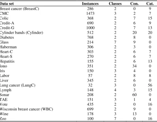
The 25 data sets used are all publicly available from the UCI Repository [12]. For a summary of data set characteristics, see Table 2 below. Classes is the number of classes, Instances is the total number of instances in the data set, Con. is the number of continuous input variables and Cat. is the number of categorical input variables.

Table 2. Data set characteristics

Data set Instances Classes Con. Cat.

Breast cancer (BreastC) 286 2 0 9

CMC 1473 3 2 7

Colic 368 2 7 15

Credit-A 690 2 6 9

Credit-G 1000 2 7 13

Cylinder bands (Cylinder) 512 2 20 20

Diabetes 768 2 8 0 Glass 214 7 9 0 Haberman 306 2 3 0 Heart-C 303 2 6 7 Heart-S 270 2 6 7 Hepatitis 155 2 6 13 Iono 351 2 34 0 Iris 150 3 4 0 Labor 57 2 8 8 Liver 345 2 6 0

Lung cancer (LungC) 32 3 0 56

Lymph 148 4 3 15

Sonar 208 2 60 0

TAE 151 3 1 4

Vote 435 2 0 16

Wisconsin breast cancer (WBC) 699 2 9 0

Wine 178 3 13 0

Zoo 100 7 0 16

4 Results

Table 3 below shows the results from the preliminary experiment. The main result is that it is clearly better to use all data for actual training, compared to re-serving some instances to be used as a validation set. Comparing TrAcc to ValAcc, TrAcc wins 15 of 25 data sets, and also obtains a higher mean accuracy over all data sets.

The explanation is obvious from the fact that using all available instances (Rand All) results in considerably higher average classifier accuracy, compared to using only 75% of the instances for the training (Rand 75%). As a matter of fact, Rand All (i.e. using a random tree trained on all instances) even outperforms the ValAcc selection strategy, both when comparing average accuracy over all data sets, and when consi-dering wins and losses.

Table 4 below shows the results from the main experiment. The overall picture is that all selection strategies outperform both J48 and Rand; i.e., picking a random tree. The best results were obtained by the selection strategy utilizing the imaginary ensemble only on the test instances, which of course is an interesting observation.

Table 3. Preliminary experiment: test accuracies

Data set TrAcc ValAcc Rand All Rand 75%

BreastC 72.7 70.6 74.2 70.3 Cmc 55.0 53.7 51.9 51.6 Colic 83.6 84.9 84.5 83.4 Credit-A 84.5 85.5 84.7 85.1 Credit-G 72.6 69.3 71.0 69.4 Cylinder 69.4 67.6 67.3 65.5 Diabetes 73.4 74.3 73.8 73.3 Ecoli 81.3 80.2 79.0 78.0 Glass 65.4 66.6 64.9 63.6 Haberman 73.3 73.6 73.4 74.9 Heart-C 76.7 77.4 76.3 75.7 Heart-S 77.3 77.7 77.0 75.2 Hepatitis 82.5 81.1 81.5 81.2 Iono 89.0 86.7 87.3 87.1 Iris 96.0 94.2 94.3 94.4 Labor 85.0 84.8 86.3 83.8 Liver 60.9 63.6 62.9 60.7 LungC 67.0 57.3 67.7 57.9 Lymph 75.7 73.5 76.0 76.0 Sonar 76.0 72.1 73.2 71.7 Tae 54.3 52.5 55.4 54.2 Vote 93.2 94.0 94.7 94.8 WBC 96.2 95.8 95.7 95.3 Wine 88.4 90.9 90.4 90.0 Zoo 93.4 90.9 91.9 88.4 Mean 77.7 76.8 77.4 76.1 # Wins 15 10 20 4

To determine if there are any statistically significant differences, we use the statis-tical tests recommended by Demšar [13] for comparing several classifiers over a number of data sets; i.e., a Friedman test [14], followed by a Nemenyi post-hoc test [15]. With six classifiers and 25 data sets, the critical distance (for α=0.05) is 1.51, so based on these tests, TeFid and AllFid obtained significantly higher accuracies than J48 and Rand. Furthermore, the difference between TeFid and TrAcc is very close to being significant at α=0.05. All in all, it is obvious that basing the selection on fidelity to the imaginary ensemble is beneficial, especially when also considering the ensem-ble predictions on test instances.

Since the most common and straightforward alternative is to simply use a decision tree, it is particularly interesting to compare the suggested approach to J48. As seen in Table 5 below, all selection strategies clearly outperform J48. A standard sign test re-quires 18 wins for α=0.05, so the difference in performance between the selection strat-egies TeFid and AllFid and J48 are significant, also when using pair-wise comparisons. In addition, both TrFid, and to a lesser degree, TrAcc clearly outperform J48. Interes-tingly enough, this is despite the fact that J48 wins almost half of the data sets when compared to a random tree. So, the success of the suggested approach must be credited to the selection strategies, rather than having only very accurate base classifiers.

Table 4. Main experiment: test accuracies

Data set J48 TrAcc TrFid TeFid AllFid Rand.

BreastC 69.9 72.7 74.8 74.8 74.8 74.2 Cmc 50.6 55.0 51.7 51.7 51.7 51.9 Colic 85.6 83.6 84.3 84.2 84.2 84.5 Credit-A 85.5 84.5 86.0 85.1 86.0 84.7 Credit-G 73.0 72.6 71.5 72.4 71.9 71.0 Cylinder 57.8 69.4 67.4 70.0 67.6 67.3 Diabetes 73.3 73.4 73.4 73.4 73.4 73.8 Ecoli 78.6 81.3 81.6 81.9 81.3 79.0 Glass 66.8 65.4 68.7 68.2 67.8 64.9 Haberman 73.9 73.3 74.0 74.5 74.2 73.4 Heart-C 75.9 76.7 76.8 77.6 76.7 76.3 Heart-S 77.0 77.3 76.7 78.1 77.8 77.0 Hepatitis 80.6 82.5 83.0 81.7 81.6 81.5 Iono 90.0 89.0 90.7 90.2 90.4 87.3 Iris 95.3 96.0 94.8 94.7 94.7 94.3 Labor 73.7 85.0 85.0 87.6 87.6 86.3 Liver 62.0 60.9 68.1 68.1 68.1 62.9 LungC 65.6 67.0 67.0 78.1 78.1 67.7 Lymph 73.0 75.7 77.7 76.4 77.7 76.0 Sonar 75.5 76.0 74.5 72.8 74.8 73.2 Tae 55.0 54.3 55.0 55.0 55.0 55.4 Vote 95.6 93.2 95.1 95.7 95.5 94.7 WBC 95.6 96.2 96.6 96.4 96.5 95.7 Wine 91.6 88.4 89.9 93.8 93.0 90.4 Zoo 93.1 93.4 91.4 97.0 96.5 91.9 Mean 76.6 77.7 78.2 79.2 79.1 77.4 # Wins 2 3 8 13 6 2 Mean rank 4.34 3.98 3.12 2.48 2.76 4.28

Table 5. Wins, draws and losses against J48

TrAcc TrFid TeFid AllFid Rand.

Wins/Draws/Losses 15/0/10 16/1/8 19/1/5 19/1/5 13/0/12

Another interesting comparison is to look specifically at selection strategies not considering test instances. After all, not all predictions are performed in bulks. Table 6 below therefore compares J48 to TrAcc and TrFid. Even now the picture is quite clear; the best choice is to select a tree based on ensemble fidelity.

Table 6. Comparing strategies not using test instances Strategy J48

TrAcc 15/0/10 TrAcc

TrFid 16/1/8 15/3/7 TrFid

Table 7 below, finally, presents the results in a slightly different way. Here, the ta-bulated numbers represent the average rank (based on test accuracy) of the selected tree among the 15 available trees. As an example, a rank of 1.00 would indicate that the suggested strategy picked the best possible tree on each fold. Here, it must be noted that when several trees obtained identical accuracies, they all got the best rank-ing, instead of an average rank. If, as an example, three trees obtained the best accura-cy, a selection strategy picking either of these trees would get a rank of 1 on that fold. A strategy picking the second best tree would then receive a rank of 4, and so on. In addition, if a selection strategy picked several trees (because they had identical scores) the ranking on that fold, for that strategy, would be the average rank of the selected trees.

Table 7. Comparing trees selected by the strategies

Data set TrAcc TrFid TeFid AllFid Rand.

BreastC 8.23 1.00 1.00 1.00 2.78 Cmc 1.50 2.75 2.75 2.75 3.55 Colic 8.42 3.33 3.50 3.50 3.80 Credit-A 7.13 3.75 6.13 3.75 7.22 Credit-G 4.25 7.25 4.25 5.75 7.65 Cylinder 5.75 7.25 4.75 6.75 7.67 Diabetes 8.75 6.50 6.50 6.50 4.82 Ecoli 4.00 3.00 2.75 3.50 7.10 Glass 7.75 2.50 2.50 3.00 7.02 Haberman 6.09 4.56 3.25 4.00 5.57 Heart-C 6.75 7.17 5.50 7.38 7.07 Heart-S 7.33 6.50 5.28 5.50 7.00 Hepatitis 4.25 4.54 4.83 5.38 5.95 Iono 6.00 2.63 3.17 3.25 7.23 Iris 3.13 1.73 1.75 1.75 3.23 Labor 6.42 6.42 3.75 3.75 5.35 Liver 10.75 3.75 3.75 3.75 7.32 LungC 6.50 6.50 2.50 2.50 6.20 Lymph 5.63 4.33 4.50 3.75 5.55 Sonar 3.75 5.00 7.42 4.75 7.18 Tae 5.25 5.50 5.50 5.50 4.82 Vote 10.59 5.69 3.50 4.25 6.73 WBC 3.83 1.50 3.00 2.38 6.78 Wine 9.00 8.25 2.00 3.50 6.43 Zoo 4.54 5.68 1.50 1.75 6.18 Mean 6.22 4.68 3.81 3.99 6.01 #Wins 5 8 13 6 2

There are several interesting observations in Table 7. First of all, no strategy suc-ceeds in always picking one of the best trees. This is a clear message that it is still very hard to estimate performance on unseen data based on results on available data. Picking the most accurate tree on training data (TrAcc), is sometimes the best option (5 wins) but, based on this comparison, it is still the worst choice overall. TeFid is

again the best selection strategy, with a mean value indicating that the tree picked by TeFid is, on average, ranked as one of the best four.

5 Conclusions

This paper shows that the predictive performance of genetically evolved decision trees can compete successfully with trees induced by more specialized machine learn-ing techniques, here J48.

The main advantage for an evolutionary approach is the inherent ability to produce a number of decision trees without having to sacrifice individual accuracy to obtain diversity. Here, each tree was evolved based on all available training data, which is in contrast to standard techniques, which normally have to rely on some resampling technique to produce diversity.

The proposed method, consequently, evolves a collection of accurate yet diverse decision trees, and then uses some selection strategy to pick one specific tree from that pool. The key idea, suggested here, is to form an imaginary ensemble of all trees in the pool, and then base the selection strategy on that ensemble. Naturally, the as-sumption is that individual trees that, to a large extent, agree with the ensemble are more likely to generalize well to novel data.

In the experimentation, the use of several selection strategies produced evolved trees significantly more accurate than the standard rule inducer J48. The best perfor-mance was achieved by selection strategies utilizing the imaginary ensemble on actual predictions, thus limiting the applicability to problems where predictions are made for sets of instances. Nevertheless, the results also show that even when bulk predictions are not possible, the suggested approach still outperformed J48.

6 Discussion and Future Work

First of all, it is very important to recognize the situation targeted in this paper, i.e., that for some reason models must be comprehensible. If comprehensibility is not an issue, there is no reason to use decision trees or rule sets, since these will almost al-ways be outperformed by opaque techniques like neural networks, support vector machines or ensembles.

A potential objection to the suggested approach is that using evolutionary algo-rithms to produce decision trees is much more computationally intense, and therefore slower, than using standard techniques. This is certainly true, but the novel part in this paper, i.e., the evolution of several trees just to pick one, could easily be run in paral-lel, making the entire process no more complex and time consuming than evolving just one tree.

Regarding the use of the same instances later used for the actual prediction when selecting a specific model, it must be noted that it is not very complicated, and defi-nitely not cheating. All we do is give each model the opportunity to vote, and then the voting results are used for the model selection. Correct test target values are, of course, not used at all during the model building and selection part.

In this study, we used GP to evolve all decision trees. The suggested approach is, however, also potentially applicable to standard algorithms like C4.5 and CART. The most natural setting would probably be quite large data sets, where each tree would have to be induced using a sample of all available instances, thereby introducing some implicit diversity.

Acknowledgments. This work was supported by the INFUSIS project (www.his.se/

infusis) at the University of Skövde, Sweden, in partnership with the Swedish Know-ledge Foundation under grant 2008/0502.

References

1. Quinlan, J.R.: C4.5: Programs for Machine Learning. Morgan Kaufmann, San Francisco (1993)

2. Breiman, L., Friedman, J.H., Olshen, R.A., Stone, C.J.: Classification and Regression Trees. Wadsworth International Group (1984)

3. Tsakonas, A.: A comparison of classification accuracy of four genetic programming-evolved intelligent structures. Information Sciences 176(6), 691–724 (2006)

4. Bojarczuk, C.C., Lopes, H.S., Freitas, A.A.: Data Mining with Constrained-syntax Genetic Programming: Applications in Medical Data Sets. In: Intelligent Data Analysis in Medi-cine and Pharmacology - a workshop at MedInfo-2001 (2001)

5. Johansson, U., König, R., Niklasson, L.: Inconsistency - Friend or Foe. In: International Joint Conference on Neural Networks, pp. 1383–1388. IEEE Press, Los Alamitos (2007) 6. Provost, F., Domingos, P.: Tree induction for probability-based ranking. Machine

Learn-ing 52, 199–215 (2003)

7. Johansson, U., Sönströd, C., Löfström, T., König, R.: Using Genetic Programming to Ob-tain Implicit Diversity. In: IEEE Congress on Evolutionary Computation, pp. 2454–2459. IEEE Press, Los Alamitos (2009)

8. Breiman, L.: Bagging Predictors. Machine Learning 24(2), 123–140 (1996)

9. Dietterich, T.G.: Machine learning research: four current directions. The AI Magazine 18, 97–136 (1997)

10. Krogh, A., Vedelsby, J.: Neural network ensembles, cross validation, and active learning. In: Advances in Neural Information Processing Systems, San Mateo, CA, vol. 2, pp. 650– 659. Morgan Kaufmann, San Francisco (1995)

11. Witten, I.H., Frank, E.: Data Mining: Practical machine learning tools and techniques, 2nd edn. Morgan Kaufmann, San Francisco (2005)

12. Blake, C.L., Merz, C.J.: UCI Repository of machine learning databases, University of Cal-ifornia, Department of Information and Computer Science (1998)

13. Demšar, J.: Statistical Comparisons of Classifiers over Multiple Data Sets. Journal of Ma-chine Learning Research 7, 1–30 (2006)

14. Friedman, M.: The use of ranks to avoid the assumption of normality implicit in the analy-sis of variance. Journal of American Statistical Association 32, 675–701 (1937)

15. Nemenyi, P.B.: Distribution-free multiple comparisons, PhD thesis, Princeton University (1963)