The Impact of Urbanization on GDP per Capita : A Study of Sub-Saharan Africa

The Impact of Urbanization on

GDP per capita

A study of Sub-Saharan Africa

Bachelor’s thesis within Economics

Author: Eva Hytenget

Tutor: Professor Börje Johansson PhD. Candidate James Dzanzi

Bachelor’s Thesis in Economics

Title: The Impact of Urbanization on GDP per capita: A study of sub-Saharan Africa

Author: Eva Hytenget

Tutor: Professor Börje Johan, Ph.D Candidate James Dzanzi

Date: June 2011

Subject terms: Sub-Saharan Africa, Urbanization, GDP per capita, City Primacy, Slums

Abstract

This thesis examines the interaction between urbanization and GDP per capita in sub-Saharan Africa. In particular, whether, increased urbanization impacts GDP per capital positively or negatively in the region. Sub- Saharan Africa, containing a total of 47 countries, remains one of the poorest regions in the world yet it has been reporting the highest urbanization rates. An interesting feature of the urbanization in the region is its degree of centrality. For this reason further examination will be done on how the size of the prime city affects GDP per capita, as well as how the prime city measured as a per-centage of urban population interacts with GDP per capita.

The econometric analysis is done using panel data regression on a GDP per capita mod-el. The model contains well known indicators for GDP growth such as gross capital formation, trade, secondary school enrollment and FDI. Also in this model is urban population in the first regression, prime city population in the second and prime city as a percentage of urban population in the third. Using the poolability and Hausman test it was established that the fixed effects panel least squares was most suited for this analy-sis.

The results from regression 1 show all variables to be significant except FDI. FDI re-mains insignificant in all the three regressions. This has also been the case in numerous studies on developing countries concerning the relationship between FDI and GDP per capita. The explanatory variable of interest, in this case urban population, shows that urbanization and GDP per capita interact positively. This means that increased urbaniza-tion will and should result in increased GDP per capita. The results from the second re-gression show that the size of the prime city as a percentage of total population is insig-nificant, however we do see that when the degree of centrality (measured by prime city as a percentage of urban population) increases there is a negative impact on GDP per capita. This would suggest that while urbanization is economically positive for the re-gion, urbanization concentrated in one or few areas dampens the effect.

Table of Contents

1

Introduction ... 1

2

Background ... 5

2.2 The Phenomenon of Over-urbanization ... 7

3

Empirical Analysis ... 11

3.1 Data collection ... 11

3.2 Descriptive statistics: Urbanization and GDP per capita ... 11

3.2.1 Descriptive Statistics: Prime city ... 14

3.2.2 Descriptive statistics: Other explanatory variables ... 15

3.3 Methodology ... 17

3.4 Results ... 21

3.4.1 Urbanization as explanatory variable of interest ... 21

3.4.2 Prime city as explanatory variable of interest ... 23

4

Analysis... 26

4.1 Discussion of Data ... 26

4.2 Discussion with reference to theory ... 26

5

Conclusion ... 29

5.1 Suggested further study ... 30

List of references ... 31

Appendix A ... 33

Figures

Figure 1-1 Urban population in Africa ... 1

Figure 1-2 Urbanization vs. HDI ... 2

Fugure 2-1 Log-Linear relationship between GDP and urban population for 1990 ... 10

Figure 3-1 SSA GDP per capita at constant prices 1980-2008 ... 12

Figure 3-2 SSA Urban population (% total) 1950-2050 ... 12

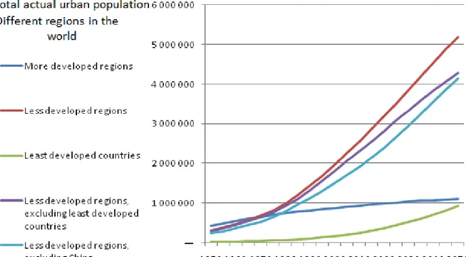
Figure 3-3 Urban Population grouped by level of development ... 13

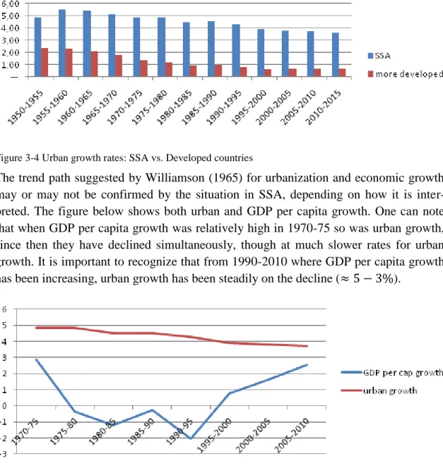
Figure 3-4 Urban growth rates: SSA vs Developed countries ... 14

Figure 3-5 GDP per capita and urban population growth rates ... 14

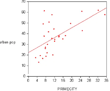
Figure 3-6 Prime city population vs. urban population (% total) ... 15

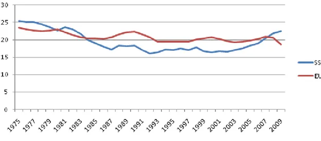
Figure 3-7 SSA vs. EU Gross capital formation as a percentage of GDP .... 16

Figure 3-8 Trade as a percentage of GDP ... 17

Figure 4-1 Urban decentralization and population per urban area vs. GNP per capita ... 27

Figure A1-1 UN world urbanization prospects ... 36

Figure A1-2 Prime city % total and % urban ... 36

Figure A1-3 Prime city % total and % urban ... 37

Tables

Table 2 Hausman's Test for Random Effects ... 21

Table 3 Fixed Effects Panel Urban population ... 22

Table 4 Fixed Effects Panel Prime city (% total) ... 23

Table 5 Fixed Effects Panel Prime city (% urb) ... 24

1

Introduction

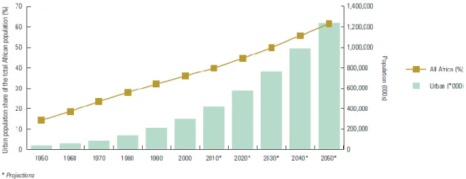
As reported in the UN’s Human development report 2010 sub-Saharan Africa (SSA) has the highest incidence of multidimensional poverty with ranges of 3% in South Africa and 93% in Niger (UNDP). At the same time SSA countries are reporting some of the high-est rates of GDP growth and urbanization (See figure below) (UN Habitat). This sugghigh-ests an uneven distribution of wealth, resource allocation and population density. The shift to urba-nization in Africa can be explained by several factors, the most recognized of these being the increase of rural-urban migration. In effect, the continent has experienced a demographic shift, facilitated mobility and education systems enable better career prospects available in larger cities. All of these combined with inefficient government policies have resulted in this mass “exodus” of rural-urban migration.

Figure 1-1 Urban population in Africa

Source: UN Habitat

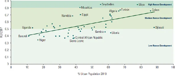
While urbanization on its own does not indicate much about the development of the country, it has been widely viewed as a sign of modernization. Countries with relatively high HDI levels have a tendency to also report high urban population (as a percentage of total popula-tion) (figure 2). This corresponds to a cross-section data study by Ambe J. Njoh (2003) for sub-Saharan Africa.

Figure 1-1 Urbanization vs. HDI

(Source: UNDP)

This urbanization, however, is skewed towards only few regions within the countries, typi-cally the prime cities. Agglomeration theory states that polarized economic activity is con-ducive for growth of industry which then feed economic growth, albeit in the short run. Effectively, the normal path of polarized economic activity is not permanent. Over time, although these centers remain the hub for economic activity, much of the prosperity of these areas defuses to the rest of the country. It would seem that this is not the case in SSA. For a majority of the countries in the region the prime city contains a major share of the urban population or large urban primacy ratio (2009 average 30-50% of urban population was in the prime city (WB)). As a result, most governments have to face the deficiency of resources verses population influx in major cities. Commonly seen across the continent are growing numbers of slums or squatter settlements and these cause problems such as increased crime rates and pollution. The heavily populous areas containing poor housing, sanitation and water facilities, are favorable environments for the spread or transmission of diseases. Argu-ably, SSA countries are experiencing problems with the increase urbanization or may be in fact dealing with a case of over-urbanization.

According to UN Habitat the general economic condition of the region has been favorable for economic growth, essentially GDP growth levels for 2010/2011 are expected to average 4%.One could then stipulate that urbanization has a role in this process of change. In devel-oping countries urban wages are much higher than in the rural areas (range from 50 – 100%). This suggests that urbanization positively interacts with increased income per capita. Higher wages in the urban areas allows for increased support to family members in rural areas (internal remittances) and education opportunities. Female participation in labor is higher in urban areas than in rural, and as studies show, female financial empowerment is more beneficial for household than males (females opt to invest in education and health) (Jiggins, 1989, Pitt and Khandker, 1998). This would suggest that the increase in urbaniza-tion should be welcomed in SSA. However, the quesurbaniza-tion is of whether the economies are at appropriate levels of development to handle this influx of urbanization. The economy may

well be able to cope, but that the problem with the said “over-urbanization” lies in poorly conceived government policies.

Contrary to developing countries, the urbanization within developed countries occurred at less rapid rates. The process for the latter was spread over many decades meaning that the transition from rural to urban governance was done with relative ease. For SSA countries where balance between urban and rural governance is concerned, the bias is towards urban. Never-the-less, this policy has done little to abate the governments’ continued struggle with the ever-increasing density of urban populations.

1.1

Purpose

The purpose of this thesis is to conduct an empirical study of the impact of urbanization on GDP per capita in sub-Saharan Africa. The posed question is: Does the level of ur-banization correlate positively with the level of GDP per capita for SSA countries? Se-condly, to what extent does GDP per capita covary with the size of a country’s prime city, measured by population of prime city as a percentage of total population and as a share of total urban population.

The choice of the region is based on the fact that sub-Saharan Africa has reported some of the highest urbanization rates in the world and yet remains one of the poorest. As-suming that urbanization is the necessary path to economic development the interest is to understand the connection between these two economic variables.

As such, the hypothesis here is that urbanization and GDP per capita are positively cor-related.

1.2

Outline

Throughout the paper specific countries will be exemplified, but for the most part the countries will be grouped (i) east SSA, (ii) west SSA, (iii) central and (iv) south SSA, or otherwise taken collectively. The intent is not to analyze each country separately but the region as a whole since the countries are not identical yet are similar enough for such a study.

The rest of the paper is organized as follows: Section 2 contains the theoretical back-ground, classical and modern theory concerning urbanization and its economical im-pacts. Over-urbanization has been separated out of the main theory so as to examine its relevance for the SSA region. Section 3 deals with the empirical part of this paper, data collection, statistical trends of all the variables used in the chosen model. The metho-dology in section 3 is extended to include steps taken in deciding which panel regres-sion would be best suited and the main findings are presented. The analysis is presented in Section 4 and finally, the conclusion in section 5 with some suggestions for further studies in section 5.1.

2

Background

There are a number of theories as to the cause of urbanization and what economic dynamics need to be present for the process of urbanizing to occur. Evidence exists that changes in GDP per capita can explain 70% of variation in urbanization (Henderson, 2002). On the other hand a great deal has been studied on how urbanization through agglomeration results in prosperous economic activity. The common variable between urbanization and GDP per capita is increased factor productivity; this section brings together the different theories concerning urbanization as well as those for GDP per capita in order to tie in the two va-riables.

2.1

Theoretical Background

Urbanization can be described as the due course (part of the process) for countries to achieve economic growth and development. It shifts the composition of national income towards more secondary and tertiary sectors and away from the volatile primary sector. This is assuming that the urbanization is accompanied by industry growth. Urbaniza-tion is essentially agglomeraUrbaniza-tion economies where increase in welfare is an outcome of the clustering of economic activity in order to gain from scale economies. The question that exists is if this is actually the case in developing countries and whether it is in fact desirable (Wheaton and Shishido, 1981).

Original urbanization theory stems from the notion that the economic markets (in the long-run) will distribute urban activity such that Pareto efficiency is reached (Lösch, 1954). Further studies suggest that at early stages of economic development countries will experience rapid urbanization but this will then taper off. The tapering off is partly due to income convergence in the different regions in the country under the assumption that internal factor mobility is well pronounced. Labor migration, either for entrepre-neurial purposes or further education and skills accumulation, will create income diffe-rentials between regions since these areas tend to have high labor participation rates. In addition, in line with agglomeration economies, there will be capital migration within countries thus creating polarized economic centers. Not only will labor and capital mi-gration create initial divergence in income for the different regions in a country, but un-evenly distributed linkages will hamper the spread of technology (Williamson, 1965). The difference between urban concentrations in countries is under two assumptions; the first is that the initial distribution is equilibrium and it is efficient in that instance. The second is that this initial equilibrium contains the tradeoffs between production costs and buyer transportation costs. The more spread the economic activity the less the transportation costs for the buyers. Yet at the same time spread increases costs per unit of production. Furthermore, the potential market size of a country possibly affects the extent of urban concentration (Wheaton and Shishido, 1981). Economists such as Fujita, Krugman and Mori (1999) stress the notion that city activity is becoming increasingly important in economic analysis as urbanization increases on a global level. There are two opposing forces that dictate the dynamics of cities, “centripetal” and “centrifugal”.

On one hand, the centripetal dynamic includes market size effects, strong labor markets and pure scale economies. These are the dynamic forces behind creating economically agglomerated centers. On the other hand, centrifugal contains dynamic forces such as immobile factors, land rents and pure scale diseconomies. The centrifugal dynamics would mean only one or few economic centers (Krugman, 1998). The classical theory of cities such as Von Thunen’s monocentric model (Beckmann, 1972) would have you believe that the latter case of dynamics is what is viewed in reality. Economic geo-graphers of today would argue that it contradicts reality.

In an environment where factors are mobile (labor and capital) and populations continue to grow the equilibrium is where you have many economic centers specialized in a par-ticular industry or production of some kind. It is argued moreover that once the popula-tion of an economy reaches a particular level, the outcome is instability in the monocen-tric theory (Fujita et al. 1999). Under the slogan “Dixit-Stiglitz, icebergers and evolu-tion”, the city agglomeration is explained further. Monopolistic competition rather than perfect competition creates scale economies opportunity. Iceberg is noted to stress that countering the forces of agglomeration are transport costs. It is such the case that at very high transport cost, economic activity is rather spread. Conversely as this falls, the ag-glomeration effects take over (however not indefinitely). Finally, evolution stated here is to establish the fact that the dynamics of cities is constantly changing. Industry will constantly be shifting towards areas of higher rates of return, as such new “cities” or economic centers are constantly forming (Fujita and Krugman, 2004).

Your typical GDP per capita growth models (Solow and endogenous growth models) specify GDP per capita growth as an outcome of saving, population growth (Solow growth model) and the interactions of the private and public sector of the country (en-dogenous growth model). Modern versions of these models including an augmented version of the Solow growth model by Mankiw et al. (1992) which puts forward, con-trary to the original version1, that income elasticity with respect to savings rate is one. Arguing further that higher savings rate will mean higher income at steady-state which in turn will mean higher total levels of human-capital (even without the change in hu-man-capital accumulation rates). Their main conclusion is that higher savings rate will increase the factor productivity of the country. Their study draws attention to the impor-tance of human capital in explaining the dynamics of GDP per capita growth (Mankiw et al. 1992). Another augmented version of the Solow model is by Nonneman and Van-houdt, 1996. They built on the foundations of the Mankiw et al. study but included in the capital variable is not only human capital along with physical capital, but m types of capital, taking into account technological “know-how”: patents, blue prints and property rights are considered.2 Their new model explains up to three-quarters of the variation in

1 _{The original assumes capital share of 1/3, therefore income elasticity with respect to savings would be} 1/2

GDP per capita3 (Nonneman and Vanhoudt, 1996). The urban growth theory put for-ward by Black and Henderson (1999) show how urban growth rate is a function of hu-man capital accumulation rates, they go further to suggest that city size grows at a 2ε rate (where ε is income elasticity with respect to human capital formation). Assuming that urbanization and GDP per capita growth are outcomes of increased productivity, then the two variables should coincide or progress in the same direction.

However, the directionality of these two variables is dual; On the one hand urbanization is an outcome of income growth fueled by increased city size and education. On the other hand scale economies, technological spillovers and well institutionalized urban growth can lead to efficient economic growth (Black and Henderson, 1999). The term institutionalized is used here to mean efficiently working urban centers governed by “good” policy and resource allocation. Without this efficacy, not only, would inequali-ties between rural and urban areas increase, but in addition that of the urban centers within themselves.

2.2

The Phenomenon of Over-urbanization

According to economists such as Hoselitz (1957) to know if a country is experiencing over-urbanization a comparison of its current level of industrialization must be made to that of the western developed countries when they were at the same level of urbaniza-tion. Of course, this would mean that there is an underlying assumption that over-urbanization was not a phenomenon experienced by Europe or the United States. While many such studies are well accredited, modern urbanization economist have steered away from historical comparisons. Instead they opt to compare the rates of urbanization to development indicators within the same country, for example GDP per capita (Brad-shaw, 1987). The argument is that over-urbanization is the result of the country not be-ing at the sufficient level of development. This means the rapid urbanization would pose a problem in a governments’ ability to curb unemployment, increase the provision of housing and other basic services (safe water supply, healthcare, education, sanitation). The theory suggests that increased urbanization would most likely mean or stem from increased industrialization. For, industries choose to locate in places that have the most economic activity. Location choice is based on availability of infrastructure, readily available capital, labor, legal markets as well as proximity to other industries in order to enjoy scale economies. As such there should be a bias towards urban development and a shift away from rural development. However, if a void exists between the level of de-velopment and rate of urbanization, the outcome is bound to be an economically ineffi-cient urban area.

The inevitable outcome of this imbalance between the rate of a country’s development and its rate of urbanization are slums or squatter settlements in or around the country’s

3 _{The “know-how” variable is measured by expenditure on R&D. Note also that this study was done on} OECD countries.

most populous urban areas (normally the prime city) (Bradshaw, 1987). The phenome-non has been viewed across SSA with examples such as Kibera in Kenya’s capital Nai-robi, Ajegunle one of many in Lagos Nigeria, Soweto in Johannesburg South Africa. UN world urbanization prospects 2009 show that these countries urban population in 2005 were 20.74%, 46.17% and 59.28% respectively. In the same year research by UN Habitat shows that of the 20.74% urban population in Kenya, 54.8% was said to be liv-ing in slums. In Nigeria this figure was as high as 65.8% and 28.7% in South Africa (see appendix A table 1 for all SSA countries). In addition the two (urban population as a % of total population and slum population as percentage of urban population) were growing at the same annual rate (see table 1). This is significant since it means every in-flux of urban population is in fact an addition to the slum population of that area. Coupling the slum situation, constant labor participation rate of between 69% and 70.6% for the years 1980-2009, and the high rate of urbanization (avg. 36%) there ap-pears to exists “over-urbanization” in the SSA region. With over-urbanization the nega-tive effects outweigh the posinega-tives by increasing unemployment, a case of excess supply of labor rather than shrinking demand.

Table 1 Urban Population and Slum Population Annual Growth Rates

SSA Country Urban population annual growth rate (%)

Slum population slum population annual growth rate (%) Mozambique 7 7 Kenya 6 6 Nigeria 5 5 Senegal 4 4 South Africa 3 3

Source: UN Habitat.org urban info. 2008 Urban Bias Theory

A study done by Lipton (1989) suggests that over-urbanization is an outcome of badly planned policies. Governments create a bias towards urbanization that the economy cannot handle, often referred to as urban bias. Lipton uses urban bias to explain the situ-ation in least-developed countries as a syndrome of “growth-with-hunger”. The argu-ment is such that polices by governargu-ments facilitate a bias of resources towards one or few regions in the country. These stimulate the rural-urban migration that causes over-urbanization. Lipton’s explanation with the urban bias theory is consistent with Hope’s (1998) argument, noting that “history matters”, in this instance referring to colonialism. During colonization, developments made in Africa were centered in ensuring produce reached markets in Europe. For this reason markets emerged in small key or port towns

across the African continent. Resources were therefore pumped into creating few eco-nomic centers, communication systems built only to serve the purpose of those centers with no regard to the rest of the country (Hope, 1998). This description can be seen in SSA countries today, higher availability of resources in urban rather than rural areas (UNDP, UN Habitat).

The Urban bias theory further suggests that the only way to solve the problem of biased resource allocation policies is to change course and concentrate on agriculture. Stating that agriculture in least developing countries has a higher capital rate of return than con-sumer production (industry). It is noted that the shift to a more urban society will pro-duce economic growth, but this is in the short run. In order to achieve sustainable de-velopment and economic growth there needs to be a bias towards agrarian investment (Lipton, 1989).

Dependency Theory

Another theory that suggests the importance of not concentrating on urbanization as a means of development, but rather insuring that agriculture become productive and rural development essential, is the dependency theory. The dependency theory, commonly explained in connection to the world systems theory, argues that the result of urbaniza-tion is the displacement of farm land for uses other than agriculture. As countries be-come dependent on economic growth through participation in world markets (i.e. inter-national trade) there is a shift from rural economic activities to urban economic activi-ties. The increased need to sustain trade and international market participation means rural practices get displaced by urban, with the only survivors being large commercial farmers (elite). All small hold farming is forced to close and its laborers move to indus-trial production (Bradshaw, 1985). Some quantitative studies on this theory have shown that dependency and economic growth/development are negatively correlated or that dependency and inequality are positively correlated (Rubinson and Holtzman, 1981). In SSA countries participation in world markets (measured by level of overall trade) has increased over the past 40 years but at a sluggish pace and totaling only approximately 20% increase for the period (WB WDI data).

Modernization Perspective

Contrary to urban bias and dependency theory, the modernity theory of urbanization po-sits that urbanization is part of the process in economic growth. Though it may over-whelm a nation ill prepared economically and policy wise, in the long-run the outcomes are favorable. Their underlying assumption is that social process is subsumed with eco-nomic development and that it is a universal pattern (Bernstein, 1971). Modernity en-tails increased industrialization, technological advancements, and the shift of economi-cal structure, all of which coincide with urbanization (Cohan, 1999). Other Moderniza-tionist go far as to say that a modernizing economy thought does this through increased industrialization is necessary in order to achieve sustainable development and environ-mental reform (Mol and Spaargaren, 2000).

In summation, there is evidence that GDP per capita effects urbanization. At the same

time agglomeration theory suggest the direction of causality is not that clear. Urbaniza-tion does in fact impact GDP per capita. The common factor between the two variables is the increase in factor productivity. The theory also shows that there are potentially negative effects of urbanization, particularly when there is a case of “over-urbanization”. This can stem from urban bias and/or international market dependency. The modernization perspective states that, the process of urbanization, while can be troublesome, is in the long-run the economically sound process to achieving sustainable development.

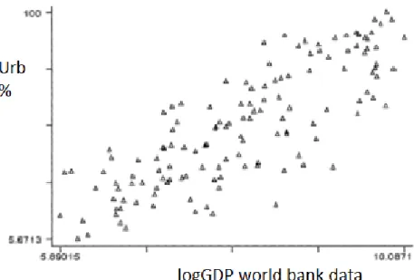
Knowing that there exits through theory and previous empirical work a positive correla-tion between the urbanizacorrela-tion and the income of a country (figure below), Henderson (2000) puts forth different ways in which the outcome does not have to be over-urbanization. To ensure “de-concentration” of urbanization: infrastructure investment, globalization and openness are solutions.

Figure 2-1 Log-Linear relationship between GDP and urban population for 1990

3

Empirical Analysis

Using the World Bank’s World development indicators data from 1970 to 2009 for all 47 SSA countries, statistical analysis of GDP per capita and urbanization is conducted in this section. Three regressions, using fixed effects panel LS is conducted for GDP per capita with the following main explanatory variables: urban population as a percen-tage of total population, prime city size as a percenpercen-tage of total population and prime city size as a percentage of urban population.

3.1

Data collection

The data presented in this paper has been collected from various sources, namely: The World Bank’s development indicators data, Penn World Tables and various segments of the UN. In particular UN Habitat, UNDP and the UN World urbanization prospects (2009 revised version).

It is important at this point to note the problems with various definitions of Urbaniza-tion. The concept of what is urban and the rural-urban divide has become more of a grey area as it changes over time (Frey and Zimmer 2001). Moreover each country has their own definition of what they constitute as urban. For example in Benin any area with more than 10,000 inhabitants is considered to be urban, in Angola this figure is 2,000 and in Botswana an area with more than 5000 inhabitants 75% of with must be engaged in non-agricultural labor would be considered urban (Cohen, 2003). This will be taken into consideration in the analysis.

The collected data on urbanization, secondary school enrollment, foreign direct invest-ment, trade as well as Gross capital formation, to be used in the regression are from WB (for definitions and measurement information see Appendix A notes 1). The data spans 40 years from 1970 to 2009. All variables where relevant are in the form of as a tage of GDP. Urbanization is measured by population living in urban areas as a percen-tage of total population, using national definitions of what constitutes as urban.4

3.2

Descriptive statistics: Urbanization and GDP per capita

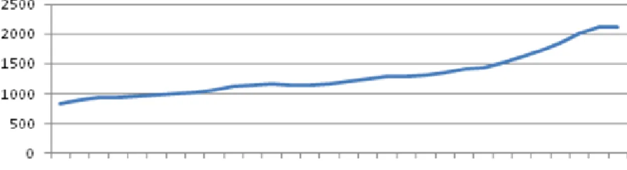
It is fitting to begin with the trends of what will be considered the dependent variable in following calculations, GDP per capita. By world standards GDP per capita in SSA has been and remains extremely low. Regardless of this fact, GDP per capita has been in-creasing over the years as the figure 3-1 below shows. The range of GDP per capita within the SSA region is large with countries such as South Africa and Botswana show-ing approximately 7500 and 8800 (constant USD prices) compared to the Democratic Republic of Congo at 231 for the year 2009.

4 _{All figures and tables, unless otherwise stated, have been self constructed using raw data from the} men-tioned sources.

Figure 3-1 SSA GDP per capita at constant prices 1980-2008

Figure 3-2 SSA Urban population (% total) 1950-2050

As the Two figures show, both variables GDP per capita and urban population as a per-centage of total population have the same upward trend. Figure 3-2 shows that urban population grew from less that 15% in 1950 to approximately 40% in 2010. More de-veloped countries have seen the same 30% increase (approx.) during these same 50, but have had better suited economies to handle the increase.

It is clear from the figure that urban population has been growing and is expected to continue 20 years from today. Furthermore, grouped countries by regions in the SSA, eastern, western and central SSA shows the same upward trend. The southern part of SSA has seen less of an increase in urban population as compared to the others (see ap-pendix A. figure A1-1). The southern region of SSA also contains the countries with the highest GDP per capita.

Figure 3-3 Urban Population grouped by level of development

It is interesting to make a comparison between the trends in SSA and the rest of the world. As noted earlier this trend of urbanization is increasingly being seen in less de-veloped countries. This would coincide with the theories that explain the urbanization process in stages, where at the beginning of economic development there should be slow urbanization, as countries move from low to medium levels of economic ment, urbanization should rapidly increase. Finally at high levels of economic develop-ment one should see a tapering off of urbanization. In Figure 3-3 one sees that for more developed regions the urbanization process has slowed and the tapering off is expected by 2020.For all other regions there is an upward trend and interestingly even for the

least developed region, urbanization has been rapidly increasing since 1990 (least

de-veloped as define by the UN GA 2001 comprises of 49 countries 34 of which are Afri-can).

Debatably, one may disagree with describing a process of urbanization based on actual population figures (as in figure 3-3) since population its self has an upward trend. How-ever, even when taking the growth rates of urban population, the fact still remains that urbanization is in fact taking place and at high rates. Seen in figure 3-4 is the growth rate compared to more developed regions (Europe, US, Australia/New-Zealand and Ja-pan). Furthermore, the data shows the rate of change for urban growth to be positive and averaging 1.76% (this should be considered high since the total population growth rate has been fairly constant around 2%). Comparatively, the rate of change for rural growth has been consistently negative from 1950 to 2010 (ranging from -0.37 to -0.87).

Figure 3-4 Urban growth rates: SSA vs. Developed countries

The trend path suggested by Williamson (1965) for urbanization and economic growth may or may not be confirmed by the situation in SSA, depending on how it is inter-preted. The figure below shows both urban and GDP per capita growth. One can note that when GDP per capita growth was relatively high in 1970-75 so was urban growth, since then they have declined simultaneously, though at much slower rates for urban growth. It is important to recognize that from 1990-2010 where GDP per capita growth has been increasing, urban growth has been steadily on the decline ( ).

Figure 3-5 GDP per capita and urban population growth rates

3.2.1 Descriptive Statistics: Prime city

In SSA countries, urbanization (urban population as a percentage of total population) and Prime city size (population of prime city as a percentage of total population) fall in the same category. Countries that have high (relatively) urbanization also have high prime city size (relatively). In 1970 the top 10 in terms of urbanization are also in the top 15 in terms of prime city size (with one outlier: Nigeria). The bottom 10 countries in terms of urbanization are also the bottom 15 in terms of prime city size. The same pat-tern holds for 2009, where the bottom 10 in terms of urbanization range between 13% and 30% also fall in the bottom 12 in terms of prime city size (ranging from 3.3% to 8.7%). This is excluding Burkina Faso which showed prime city size increase by ap-proximately 520% (but only 350% increase in urban population). For the top 10 urba-nized countries in 2009, all except Nigeria and South Africa fall in the top 15 prime city

size (note that these two countries are the wealthiest in the region). Some of the num-bers are staggeringly high, with countries such as Angola, Republic of Congo and Libe-ria showing 35%, 32% and 24% of the population as living in the prime city. Caution on the interpretation of this should be taken as these countries have civil unrest in common (For example in Angola, rebel activity was mainly in rural areas, therefore this could explain the urban population influx). Figure 3-6 below shows the relationship between urbanization and prime city size (both measures by their population with respect to total population).

Figure 3-6 Prime city population vs. urban population (% total)

The comparison between urbanization and prime city as a percentage of urban popula-tion is rather different from the preceding discussion. While countries in SSA with low urbanization show low prime city size as a percentage of total population, the prime city as a percentage of urban population is high. The reverse is the case for countries with high urbanization. These countries show lower city primacy as a percentage of urban population.

3.2.2 Descriptive statistics: Other explanatory variables

Capital formation: As discussed in the theoretical background, capital formation both physical and human (education) are of great importance in determining GDP per capita as well as urbanization. Gross capital formation (known from here on as just invest-ment) has in both regions (EU and SSA) remained between 25% and 15% of GDP. In absolute terms there is an upward trend which is consistent with GDP per capita growth being dependent on the “whole” history of capital accumulation (Solow 1962). SSA countries however, have been lagging behind other developing regions in terms of not

only domestic investment but foreign direct investment. All developing regions have in the recent decades seen major increases in FDI, however while SSA shows over 200% increase since 1980-89 and 1990-99, other regions, namely Asia and south America have seen growth in FDI of up to 900%. This fact may be in relation to the low domes-tic investment rates. As mentioned, EU and SSA have had the same investment as the percentage of GDP, but of course it matters how high the GDP is.

Figure 3-7 SSA vs. EU Gross capital formation as a percentage of GDP

Human capital, measured in this paper by education (specifically secondary school enrollment), is alarmingly low. The average for the region in 2008 was recorded at 34% only a 12% increase since 1991. Looking at individual countries, one can make infe-rence that those with relatively high GDP also have high secondary enrollment. At least for Botswana (which has the highest GDP per capita in the region) this seems to be the case with secondary enrollment at heights of 81%. Mauritius also on the top end of GDP per capita has high enrollment percentage of 87%. Contrary to one of the lowest GDP per capita countries, Niger in 2009 only reported 11% of its population as being enrolled. This is dismal for a region that is boasting some of the highest urbanization rates in the world. Of course there are other forms of human capital, for example the ur-ban areas may not have secondary school educated labor but rather labor trained specif-ically for particular industries. Without further information on this alternative human capital accumulation, no conclusions can be drawn from this.

Trade as a percentage of GDP is one of the 5 explanatory variables in the model pre-sented in this paper. It has been widely used in explaining economic growth and has been found to be positively related to GDP per capita. It has been increasing since 1960, but markedly not by drastic rates. Trade as a percentage of GDP is the sum of all im-ports and exim-ports divided by GDP, therefore this sluggish growth could be due to low imports (this could be interpreted in different ways) or low exports. Most of SSA coun-tries are exporters of primary (or raw materials) goods, a sector extremely volatile to ex-ternal conditions.

While it is possible to speculate on correlations between different variables, a more sol-id inference can only be made using more statistically complex methods. What can be taken away from this section is that all explanatory variables and GDP per capita have had a growing trend.

Figure 3-8 Trade as a percentage of GDP

3.3

Methodology

Three regressions will be run. Firstly, to find out what impact urban population has on GDP per capita. Secondly, the prime city size, as a percentage of total population will replace urbanization as an explanatory variable in determining GDP per capita. Finally, the third regression contains prime city size as a percentage of urban population.

Before the panel regressions are run, there is need to test how the intercept and the error term will be handled. In essence the choice in using panel data should help correct for heterogeneity and multicollinearity. With the former, panel data deals with this by ac-counting for omitted variable which is not the case in time series or cross-sectional data. Multicollinearity is dealt with by creating more variation both between the different va-riable and across time. The most profound advantage of using panel data is that it is eas-ily used for dynamic analysis (Kennedy, 2008).

From the three forms of panel data (Pooled, Fixed effect or Random effect) two tests were performed to decide which is to be used. Since the pooled version assumes equali-ty in intercepts of all cross-sections the first step is to determine the poolabiliequali-ty of the data. The null hypothesis in this instance is: all the intercepts are equal. If the intercepts are equal, the pooled regression should suffice in the analysis. Intuitively with the said variables being used in this regression, it is highly unlikely that is the case. However for verification the poolability test was conducted. The following regressions were run in EViews, equation (1) for pooled panel and the two-way fixed effects panel equation (2), with urbanization as the explanatory variable of interest:

Equation (1)

Equation (2)

where,

α= intercept

Urbit= Urban population as a percentage of total (cross-section I and period t)

GCFit= Gross Capital formation as a percentage of GDP

Tradeit= Total trade as a percentage of GDP

Fdiit= Forgien direct investment as a percentage of GDP

Sec.rollit= Gross secondary school enrollment

Three part error term

αi = group fixed effect (controls for permanent differences between the groups)

λt= time fixed effects (common impacts on all groups by varying over time)

µit= idiosyncratic error term

with the null hypothesis:

the poolability test is constructed as follows:

where RRSS is the restricted residual sum of squares taken from the pooled panel re-gression and the URSS is the unrestricted residual sum of squares from the fixed. The results of the F-test were as follows (Baltagi, 2005):

at this point the H0 that all intercepts are equal is rejected5. These different intercepts are

explained by the fact that apart from calculable variables such as total population, GDP per capita or gross capital formation, there can exists other heavily embedded institu-tional factors or geographical factors that make the intercepts different. For this reason the fixed effects or random effects panel formation is of great assistance (Kennedy, 2008).

The fixed effects approach: The data is transformed and the LS regression can be con-ducted (without an intercept) to give the desired fixed effects estimators from the fol-lowing:

The disadvantage of this method is that in creating the dummy variable you lose all but 1 of the degrees of freedom per cross-section. If there was a way to avoid this loss of degrees of freedom then the estimators would be more efficient. The second disadvan-tage that occurs at the point of transformation, subtraction of the observations average in each cross-section means that if there are time-invariant variables these get eliminated. This does not pose a problem in the panel regression to be presented here. Much in the same as the fixed effects approach, the random effects approach transforms the data. This approach assumes the intercepts to come randomly from a pool of intercepts. In this way the intercept is treated as the error term. The regression therefore has two ran-dom variables, the intercept and the normal error term making a component error term. Estimated generalized least squares (EGLS) is used to transform the data to form a spherical variance-covariance matrix after which Swamy and Arora estimators on the EGLS random effects model are obtained:

where µ is the random intercept and is the composition of the intercept and the normal error term6. Swamy and Arora estimators from the regression are obtained from:

where

5 _{Complete EViews output on the pooled panel can be seen in Appendix B} 6 _{Complete EViews output on the random effects can be seen in Appendix B}

Fixed effects approach vs. Random effects approach: The random effects results in more efficient estimators because it saves degrees of freedom lost during the transfor-mation in the fixed effects approach. The random approach fixes the problems faced in using the fixed effects approach however the random approach can only be used in cer-tain circumstances. The problem with the random approach is that the slope estimator tends to be overstated. Increase in the slope estimator is determined by a) increase in the explanatory variable (e.g. urbanization) and b) the increase in the dependent variable (GDP/cap). However in the random approach the dependent variable (GDP/cap) in-creases due to two factors the increase in the explanatory (urban population) and the likeness of a larger intercept. The EGLS cannot distinguish between the two and there-fore include both increases in the dependent variable. This is not the case for the fixed effects because in that instance dummy variables are assigned. In the random effects, the intercept is assumed to be random therefore the error term becomes inflated and will move with the explanatory variable (as urbanization increases then so does the compo-site error term) resulting in correlations between the two. It is for this reason that the es-timator is then considered biased. Technically the tradeoff between the two is that the fixed effect is always unbiased but the random effects approach results in greater

effi-ciency (Kennedy, 2008). In addition to the effieffi-ciency of the random effects model, is

that the estimators it account for the weighted average of both the within and between variation in the sample. There are two types of variation in the panel data, within or be-tween. It is also important to note that in the fixed effects the variation is within each cross-section of data and does not take into account the variation between the different cross-sections. When a simple pooled panel regression is done the estimators are un-weighted averages of the within and between variations where as the random effects es-timators are a weighted average (Hsiao, 2003).

While it seems the random effects should produce the best estimators for analysis pur-poses, it is also the source of the bias. The random effects should only be used if there is confidence that there is no correlation between the explanatory variable and the error term. This can be tested using the Hausman test for independence. Regardless of the null hypothesis the fixed effects is always unbiased but the random effects is only un-biased if the null is not rejected. It turns out that if the null for the random effects is not rejected then the estimators in both cases should be equal. Conducting the Hausman test under the hypothesis:

Table 2 Hausman's Test for Random Effects

Variable Fixed Random Var, (Diff) P.Values

URB 0.02 0.02 0.00 0.00 LOG(GCF) 0.16 0.16 0.00 0.45 LOG(TRADE) 0.28 0.31 0.00 0.00 FDI 0.00 -0.01 0.00 0.00 SEC, roll 0.02 0.02 0.00 0.00 Test summary Chi-square statistic 77.75 Degrees of freedom 5.00 P.Value 0.00

The table shows the significance of the test, with a chi-squared statistic of 77.75 and 5 degrees of freedom the H0 is rejected at any level of significance since 77.8 exceeds any

critical value. As such the error terms and explanatory variables are correlated making the estimator from the random effects biased. It is also shown in the output that the es-timators of the fixed and the random are different from each other, this would be consis-tent with a H0 rejection.

The same tests were conducted for the panel data on the two prime city size measures (as a percentage of total population and as a percentage of urban population). Once again, fixed effects panel was chosen as best suited for the analysis.

Having conducted the two tests, poolability and Hausman, the best panel analysis to be used in this instance is the fixed effects panel. The next section describes the results from the two-way fixed effects LS panel run in EViews.

3.4

Results

This section gives the fixed effects panel LS regression results for the three regressions. Regression 1 contains urban population, regression 2 contains prime city population (as a percentage of total population) and regression 3 contains prime city as a percentage of urban population.

3.4.1 Urbanization as explanatory variable of interest

For practical reason the model using urbanization is re-stated here as follows:

where GDP per capita is taken annually from 1970-2009 at constant USD prices, urban population is as a percentage of total population, secondary enrollment is the total per-centage of enrollment regardless of age, FDI, investment(GCF) and trade are all as a percentage of GDP.

The panel LS output was as follows:

Table 3 Fixed Effects Panel Urban population

Dependent variable: Log(GDP per Capita)

Variable Coefficient Std, Error t-Statistic Prob.

Urb 0.0146 0.0021 6.8012 0.0000 Log(GCF) 0.0515 0.0245 2.1065 0.0355 Log(trade) 0.1287 0.0323 3.9897 0.0001 FDI -0.0013 0.0017 -0.7329 0.4639 Sec, Roll 0.0101 0.0011 8.9328 0.0000 Constant 5.7118 0.1333 42.8388 0.0000 R-squared 0.9510 F-statistic 184.6946 Prob. (F-stats) 0.0000 No, of obs. 916.0000

From the regression we see that the coefficient for urban population is 0.0145 and is significant. This means a one percent change in GDP per capita can be explained by a 1.4 percentage point change in urbanization. The other variables also show consistency with theory; investment, trade and secondary school enrollment are positively related to GDP per capita (with 5, 1.3 and 1.01percentage points respectively) and are significant. Noted, FDI shows to be negatively related to GDP per capita, and is insignificant at a probability of 0.46. However this could be for several reasons. There is the likelihood that FDI is correlated with one or more of the other variables, namely trade and invest-ment (Gross capital formation).

The R-squared of this regression is high at 95%7, this suggests the model presented here explains the relative changes of GDP per capita and has the strength for prediction.

7 _{Using EViews for this regression means the squared is the combination of the within and between} R-squared and thus this could be the reason for such a high figure.

ically in economic empirical work, it is rare to get such a high R-squared. Therefore there is cause to believe the model is tainted with multicollinearity. The rule of thumb is that if the independent variables are correlated above 0.80 then there is reason to be concerned (Leahy, 2000). However, this does not take away from the analysis8, cause for concern would be if a large number of the coefficients were insignificant and the R-squared was still reporting high “goodness-of-fit”.

3.4.2 Prime city as explanatory variable of interest

The models using prime city size is formulated in the same way as equation (2) except replacing urban population with the different measurements of primacy. The model thus becomes as follows: And

where, the variable Prime is the prime city size as percentage of total population for 29 countries, from 1970 – 2009. P.city is the prime city size as percentage of urban popu-lation, also for 29 countries from 1970 - 2009. Note that the previous section contained all 47 SSA countries. The panel LS output with Prime was as follows:

Table 4 Fixed Effects Panel Prime city (% total)

Dependent variable: Log(GDP per Capita)

Variable Coefficient Std, Error t-Statistic Prob.

Prime -0.000726 0.007469 -0.097251 0.9226 Log(GCF) 0.106335 0.027385 3.882917 0.0001 Log(trade) 0.116012 0.033542 3.458675 0.0006 FDI -0.009668 0.002318 -4.170530 0.0000 Sec, Roll 0.004030 0.001555 2.591453 0.0098 Constant 5.983872 0.145219 41.20592 0.0000 R-squared 0.924816

F-statistic 92.43061

Prob. (F-stats) 0.000000

No, of obs. 597,0000

The regression shows the prime city size as a percentage of total population to be insig-nificant in relation to GDP per capita. The other variables still show consistency with theory; investment, trade and secondary school enrollment are positively related to GDP per capita (with 10, 11 and 9 percentage points respectively), they are also significant. The coefficients are inflated compared to the regression with urbanization, this could be due to the fact that one variable is dropped (Prime is insignificant therefore we have on-ly 4 explanatory variables). Noted, as in the 1st regression, FDI shows to be negatively related to GDP per capita, but in this case FDI is significantly different from zero. The model’s R-squared is high at 92%, this suggests the model presented here explains the relative changes of GDP per capita and that prime city size is insignificant.

The panel LS output with P.city was as follows (with prime city size measured as a per-centage of urban population):

Table 5 Fixed Effects Panel Prime city (% urban)

Dependent variable: Log(GDP per Capita)

Variable Coefficient Std, Error t-Statistic Prob.

P.city _{-0.019717 0.002476 -7.962207} 0.0000 Log(GCF) _{0.068145 0.026481 2.573344} 0.0000 Log(trade) _{0.064675 0.033270 1.943946} 0.0104 FDI _{-0.008968 0.002219 -4.040698} 0.0525 Sec, Roll _{0.002349 0.001527 1.537900} 0.0001 Constant _{6.986059 0.174493 40.03626} 0.0000 R-squared 0.933837 F-statistic 101.2181 Prob. (F-stats) 0.00000 No, of obs. 597,0000

This regression shows that prime city size as a percentage of urban population is nega-tive in relation to GDP per capita. Because the coefficient is significantly different from zero it can be suggested that in SSA a 1% increase in P.citychanges GDP per capita by – 1.9 percentage points. R-squared is once again high and all other variables are consis-tent with theory as in the other two regressions.

4

Analysis

From the results we find inference between GDP per capita and urbanization. The re-sults show a model of good-fit and all apart from FDI have been consistently signifi-cantly different from zero. There is consistency in the three regressions concerning a high R-squared, which is high in all three regression (ranging from 92% to 95%).Since 4 out of 5 variables in the regressions are significant there is no cause to believe multi-collinearity takes away from any analysis or inference that can be made. There are two main issues that can be discussed in this section: the concerns with data and the relev-ance of the results concerning the theory presented in the background.

4.1

Discussion of Data

As noted earlier what is considered as “urban” for the World Bank data is based on na-tional definitions that vary. In this sense one could argue that acknowledging an area of only 2000 inhabitants as urban, greatly distorts the reality of the situation. That in fact the agglomeration process is not happening therefore neither would its economic advan-tages. As such it would be expected that urban areas in SSA do not portray the econom-ic advantages of urbanization. However, it could be argued that using national defini-tions gives the relative changes that would not be captured by a set benchmark (for ex-ample 20,000 inhabitants). The data shows that urban population is heavily concentrated in few regions within the countries (prime city size) therefore this shows that the urba-nization process is occurring and it may be the disparity between government resources and the rate of urbanization that has been causing slum or squatter settlements. Needless to say, there is not enough information to state this as a fact.

It is worthy of keeping in mind the lack of complete data for the region causing an un-balanced regression especially when considering prediction strength or policy recom-mendations (technically with 47 cross-sections and 40 periods the observations should total 1880, but as seen in the output the regression was run on 44 cross-sections totaling 916 observations). There is however confidence in the robustness of the models. In par-ticular the models containing urban population and prime city as a percentage of urban population, since all forms of the panel regressions (pooled, fixed effects and random effects) show the respective coefficients not only with the correct sign but that they are all significant.

4.2

Discussion with reference to theory

A number of theories have been outlined explaining how and why countries become ur-banized. Also in which circumstances the positive aspects of urbanization would not be viewed.

From the data and the regression we find that urbanization can explain the dynamics in GDP per capita, this is consistent with the theory outlined in this paper. Pointed out is that GDP per capita is conducive to increases in total human capital accumulation, to the extent that an urbanizing economy has a better educated society then the connection

between urbanization and GDP per capita is intuitive. As suggested in the theory, coun-tries go through different stages of urbanization. At low levels of income urbanization growth is low, rapid at medium to high levels and finally at high levels of income urba-nization growth slows down, the direction of causation being GDP per capita to urbani-zation. The argument here is that there is a feedback effect. As seen from the regres-sions urbanization can account for variations in GDP per capita in SSA. We see from the data that urbanization and GDP per capita have been simultaneously increasing from 1970-2009. The regression tells us that urbanization could be causing GDP per capita increase by 1.4 percentage points.

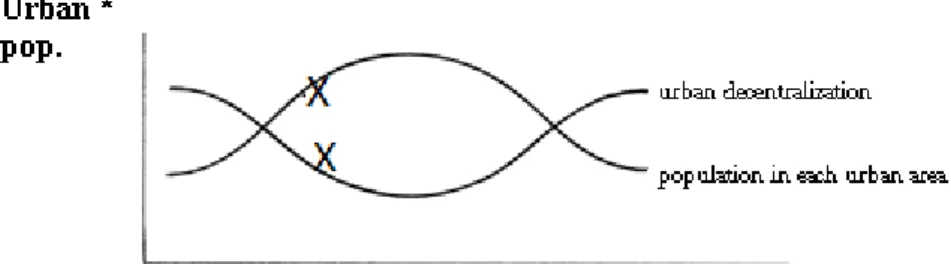
Utilizing a graph by Shishido and Wheaton (1981), the situation in SSA could corres-pond to the section marked X on the figure below. As this would represent the stage at which, while GDP per capita is increasing the population in urban areas is increasing and the degree of centrality is also increasing. From the descriptive data section we see that centrality, as measured by percentage of urban population living in the prime city, is present in SSA. There is a large portion of total urban population living in the prime city.

Figure 4-1 Urban decentralization and population per urban area vs. GNP per capita

(* the horizontal axis is a combination of the H index (measuring urban decentralization) and market po-tential (measured by S/GNP per capita) to show the population of each urban area)9

From the regression on size of the prime size (compared to total population), it is shown that the size of the prime city does not have any significance to GDP per capita. Interes-tingly, in SSA countries a large proportion of the urban population lives in the prime city and since urbanization has a positive effect on GDP per capita, one would expect to see the same results here. However, in connection to the theory, this could be due to the fact that the population of a city alone does not say anything about the market effects, scale economy opportunities and labor markets which are the driving forces for positive economic agglomeration. In another sense it could mean that urbanization of one partic-ular area is not of relevance to GDP per capita, but rather total urbanization levels of a country.

The third regression that uses prime city population as a percentage of urban might be a good way of showing that the monocentric model is flawed. Specifically, with econom-ic instability when population gets large. We see that urban population is increasing and at the same time these are concentrated in one central economic hub. The regression tells us that this increased degree of centrality has a negative dynamic effect on GDP per capita. As prime city size as a percentage of urban population is negatively corre-lated to GDP per capita, a 1% increase in the P.city variable changes GDP per capita by – 1.9 percentage points.

In the line of thought concerning over-urbanization the results suggest that there are positive effects of urbanization on GDP per capita, but if not controlled or governed correctly it can hamper economic growth. From the study here, what can be said it that urbanization can explain variation in GDP per capita, at least by 1.4 percentage points and that in the past 40 years urbanization has influenced GDP per capita positively in the SSA region. It can also be said, however with caution, that “over-urbanization” is taking place in SSA. This is inferred from regression 3. Moreover it can also be drawn from the fact that a large proportion of urban population live in slums (Appendix A for figures on this) and as discussed in the section on urban bias, the annual growth rate of urban population is exactly equal to the annual growth rate of slum population. This would suggest the disparity in government resources verse urban population influx. The results showing the positive impact of urbanization on GDP per capita coincides with agglomeration theory, that there are large economic opportunities that can be ex-ploited by the concentration of economic activity. The tricky aspect of the results how-ever, is that the primacy of a city predisposes the agglomeration process. This means that the processes of primacy is necessary for agglomeration economies to be achieved, yet at the same time regression 3 tells us that this concentration has a negative impact on GDP per capita. In essence primacy and agglomeration are interdependent.

5

Conclusion

The basis of the study was in conjuncture to the reported rapid rates of urbanization in the SSA region accompanied by rising GDP per capita and economically favorable growth rates.

Using fixed effects panel data on urban population, a regression was run on the impact of urbanization on GDP per capita for SSA countries over the past 40 years. The regres-sion showed that urbanization impacts GDP per capita positively. The robustness of the model stems from the fact that in all three forms of panel regression the result remains the same. Therefore there is no question that the growth of urbanization in SSA is a pos-itive factor for GDP per capita growth. This coincides with the theory discussed in sec-tion 2. The second purpose of this paper was to find out if there is a connecsec-tion between the prime city size (measured as a percentage of total population) and GDP per capita. The results from the regression, using the same model but replacing urban population with prime city size, showed that prime city size was insignificant in relation to GDP per capita. As discussed in the Analysis this was unexpected, however not unexplaina-ble. It is argued here that this could be due to the fact that the size of a city via its popu-lation does not show the economic aspects present in the city. In particular, economic aspects that would result in positive economic agglomerative activity, leading to in-creased income.

The concerning factor is that at the same time as the region is experiencing rapid urba-nization, living conditions seem to be dire. Growing slum and squatter settlements in or around cities, leaded one to believe that the urbanization process is having negative ef-fects. The urbanization taking place in SSA is concentrated, particularly in the prime city. From the third regression, using prime city size as a percentage of urban popula-tion, it is found that there is a negative impact on GDP per capita. This means that the increase in urbanization is positive for GDP per capita, but is negative for GDP per ca-pita if it is only concentrated in one area of a country. The theory in section 2 also cor-responds with this notion that a monocentric model of agglomeration would result in economic instability, especially as population increases.

Data shows that for SSA countries growth in urban population is concentrated in the prime city, also that it is exactly equal to growth in slum population. This coincided with the regression 3 that shows that increased urbanization in the prime city relative to elsewhere in the country is negatively correlated with GDP per capita. The definition of slum areas is such that people are forced to live in cramped spaces with no durable housing, insufficient water supply, insufficient sanitation etc. Therefore it would be un-likely that the increase of such areas would impact the economy positively, for example through increased labor participation. The question however, is that knowing urbaniza-tion increases GDP per capita for the region, then should this negative impact be ac-cepted as part of the process in achieving economic development in the long-run or should policies be put in place to facilitate urbanization in a more balance manner across the countries.

5.1

Suggested further study

Lacking from this study was the availability of data. In particular those that would indi-cate economic activity that is favorable for agglomeration. Without information on in-dustry growth in cities for the region it is difficult to have studies such as Henderson and Blacks 1999 study concerning agglomeration rates and how this translates into posi-tive urbanization.

It would be interesting to analyze the difference of urbanization impacts on GDP per capita for different regions worldwide but this is beyond the scope of this paper.

Slum data, could be used to study the growth of slum over time in relation to urbaniza-tion growth. This could give a better view of whether over urbanizaurbaniza-tion is in fact occur-ring in the region. Furthermore one could compare income levels in the slum areas rela-tive to rural areas to establish if in fact people remain better off with urbanization de-spite the sub standard living conditions of slum areas.

Appendix

List of references

Baltagi B. H, Econometric Analysis of Panel Data, Third Edition, John Wiley & Sons Ltd, England 2005

Beckmann M. J, Von Thunen Revisited: A Neoclassical Land Use Model, Swedish Jour-nal of Economics Vol. 74 No. 1, 1972

Bernstein H, Modernization Theory and the Study of Sociological Development, Journal

of Development studies, 1971

Black D. and Henderson V, A Theory of Urban Growth, Journal of Political Economy Vol. 107 No.2, 1999

Bradshaw Y. W, Urbanization and Underdevelopment: A global study of

moderniza-tion, urban bias and economic dependency, American Sociological review, Vol. 52

No.2, 1987

CohenB, Urban Growth in Developing Countries: A Review of Current Trends and a

Caution Regarding Existing Forecasts, National Research Council, Washington DC,

World Development Vol. 32 No. 1, 2004

Fujita M, Krugman. P, Mori. T, On the evolution of hierarchical urban systems, Euro-pean Economics Review Vol. 43, 1999

Fujita M and Krugman P, The New Economic Geography: Past, Present and Future, Papers in Regional Science Vol. 83 No. 1, 2004

Frey W.H. and Z. Zimmer, Defining the City, In: R. Paddison (ed.) Handbook of Urban

Studies. Sage Publications, London, 2001

Henderson V, Urbanization in developing countries, The World Bank Research observ-er Vol. 17 No. 1, 2002

Hope K. R, Urbanization and Urban Growth in Africa, 1998

Hoselitz. B . F, Urbanization and economic growth in Asia, Journal of economics de-velopment and cultural change Vol. 6 No. 1, 1957

Hsiao C, Analysis of Panel Data, 2nd Edition, Published by the University of Cam-bridge, 2003

Jiggins J, How poor women earn income in sub-Saharan Africa and what works against

them, World Development Vol. 17 No. 9, 1989

KennedyP, A guide to Econometrics, 6th Edition, Blackwell Publishing, 2008

Krugman. P, What is new about economic geography, Oxford Review of Economic Pol-icy, Vol. 14 No. 2, 1998

Leahy, Kent. Multicollinearity: When the solution is the problem, In O. P. Rudd and J. Wiley (Eds.), The Data Mining Cookbook. New York: Chicheste, 2000

Lipton. M, Why poor people stay poor: Urban bias in world development. Hampshire, UK: Avebury, 1989