Amplification criterion of gradually varied, single peaked waves

AMPLIFICATION CRITERION OF GRADUALLY

VARIED, SINGLE PEAKED WAVES

by

JOHN PETER JOLLY

and VUJICA YEV

JEVICH

December 1971

AMPLIFICATION

CRITERION

OF

GRADUALLY

VARIED

,

SINGLE

PEAKED WAVES

by

Jo

hn

Peter Jolly* and Vujica Yevjevich**

HYDROLOGY PAPERS COLORADO STATE UNIVERSITY FORT COLLINS, COLORADO 80521

• Asslnant Professor. Department of Civil Engineering, Faculty of Science and Engineering, University of Ottawa, Ottawa, Canada. ••Professor of Civil Engineering, Colorado State University, Fort Collins, Colorado.

CHAPTER

2

3 4 5 6 ,·

T

ABL

E

OF CON

TEN

T

S

LIST OF FIGURES

LIST OF SYMBOLS

ACKNOWLEDGMENTS, ABSTRACT

INTRODUCTION

LITERATURE REVIEW

THEORETICAL CONSIDERATIONS

3.I

Uniform

Flow

. .

.

. . . .

3.2

Math

ematica

l Development

of

Gradually Varied

Flow Equations

.

.

.

.

. .

.

. .

.

.

.

.

NUMERICAL SOLUTIONS OF GRADUALLY VARIED F

LOW

EQUATIONS

4.I

Intr

o

du

ctio

n

. .

.

.

. .

4.2 Characteristic Grid Scheme

4.3 Specified Int

ervals

Scheme

4.4 Comparisons of Solutions Obtain

ed by

the

Chara

c

teristic Grid

an

d Specified

I

ntervals Schemes

4.

5

Accuracy

of

Specified

I

nterval

s

Scheme in

Simulating Supercritical Flows

4.5 .1

Intr

o

duction

4.5.2 Grid

s

ize

. . .

.

4.5

.3

Integration technique

s

4.5

.4

Flow

acce

leration

co

n

side

ration

s

AMPLIFICATION CRITERION

5.I

Introduction

. . .

. .

5.2

B

ou

nd

ary

Conditions

5

.2.

1 Initial

co

nditions

5.2.2

Inlet

con

diti

o

ns

.

5.3

Flow Simulations

. . .

5.3.1 Choice of

width

-

depth ratio

5.3.2

Amplification criterion

. .

5.4 Some

Characteristics of Supercriti

c

al Gradually

Varied

,

Single P

eaked

Wave

s

CONCL

US

IONS

REFERENCES

PAGE

iv

vii

viii

3

5

5

5 9 9 9 9

11

12

1

2

14

16

22

2

4

24

24

24

2

4

2h

26 26

28

37

38

LIST OF FIGURES

4.1

Families of

Characteristic

Curves

for both

Subcritical and Supercritical

Flows

4.2 4.3 4.4 4.5 4.6 4.7 4.8 4.9 4.10 4.11 4.12 4.13 4.14

Grid

for

the Solution by Cha

r

acteristic

Grid Scheme

Grid

for

the Solution by Specified

Intervals Scheme

Comparison

of

Solution

by

Characteristic Grid and

Specified

Int

ervals Schemes

.

.

. .

. .

.

.

.

.

.

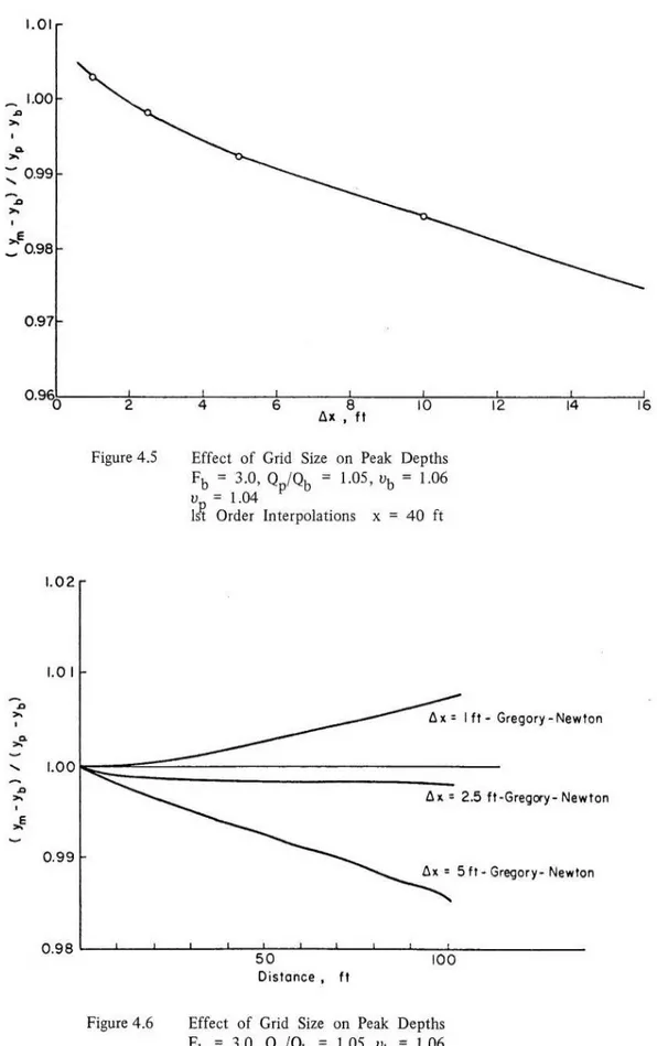
Effect of Grid Size on

Peak Depths

Fb

= 3.0,

Qp

/

Qb

=

1.05 '

Ub

=

1.06 '

Up=

1.04 I st

Order

Interpolations

x

=40ft

.

. .

. .

.

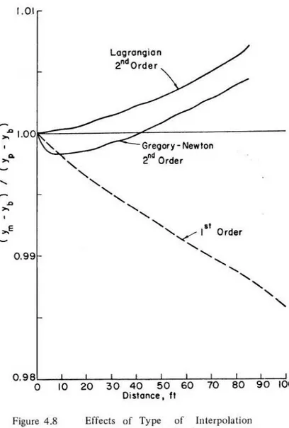
Effect

of

Grid

Size on Peak D

epths

Fb

=

3.0 '

Op/Ob =

1.05 ' Ub

=

1.06 '

Up=

1.04

Effects of

Type

of

I

nterpolation

Equation

on

P

eak

Depths for an

Attenuating Wave

Fb =

1.5 '

Op/Ob

=

1.05 '

Ub

= 0.53 '

Up

= 0.52

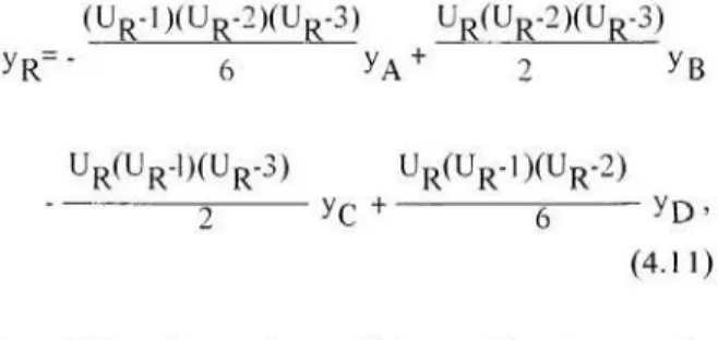
Effects of

Type

of

Interpolation

Equation

on Peak

Depths for an Amplifying

Wave

Fb =

3.0 '

Op

/

Qb =

1.05 '

Ub

= 1.06 '

Up=

1.04

Effects

of

I

ntegration Technique

on

Peak

Depths

for

an

Attenuating

Wave

Fb

=

1.5 ,

Qp/Ob

=

1.05 ,

Ub

=

0·.53 '

Up=

0.52

Effects

of

Integration Technique on Peak

Depths

for an Attenuating

Wa

ve

Fb

=

1.5 ,

Op/Ob

=

1.30 ,

ub

=

0.53 ,

up= 0.48

Effects

o

f

I

ntegration Technjque

on Peak

Depths

for

an Amplifying

Wave

Fb =

3.0 '

Op

/

Ob = 1.05

'

Ub

=

1.06 ,

Up= 1.04

Effects

of Integration Technique

on Peak

Depths

for an

Amplifying Wave

Fb

= 3.0

'

Op/Qb

=

LOS ,

Ub = 1.06

'

Up=

1.04

Effects

of I

ntegration

Technique

on

Peak

Depths

for an

Attenuating

W

ave

Fb

= 3.0 '

Op/Ob

= 1.30 ,

Ub = l.Q6

'

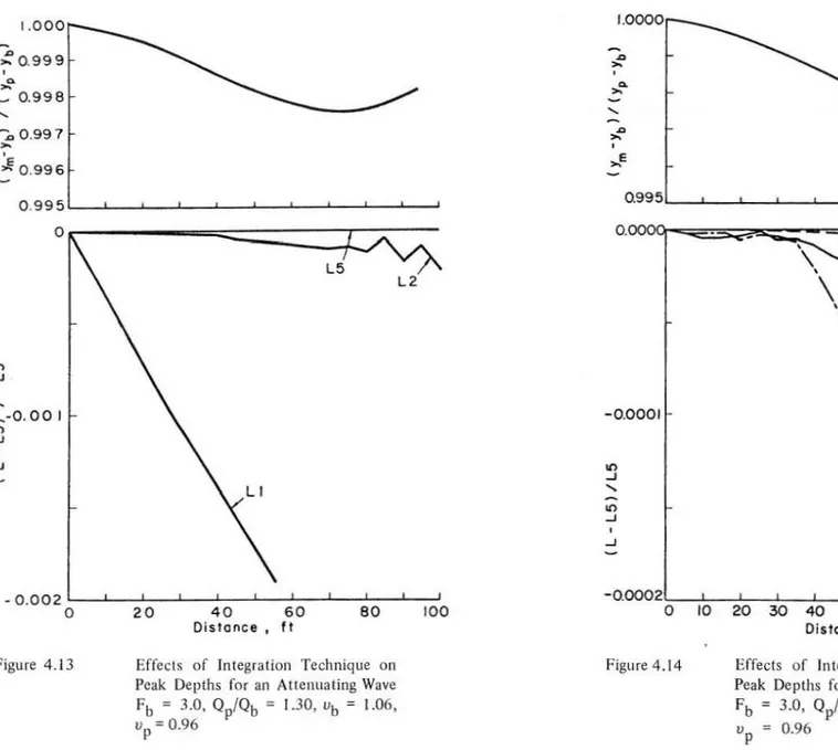
Up= 0.96

Effe

c

ts

of Integration Technique on

Peak Depths

for

an

Attenuating

W

ave

Fb

= 3.0

,

Qp

/

Qb

=

1.30,

Ub =

1.06 ,

Ub

=

0.96

Page

10 10

I

3

13 15

IS

17 19 19

20

20

21 21

4.15 4.16 4.17 4.18 5.1 5.2 5.3

5.4

5.5 5.6 5.7 5.8 5.9

LIST OF FIGURES (continued)

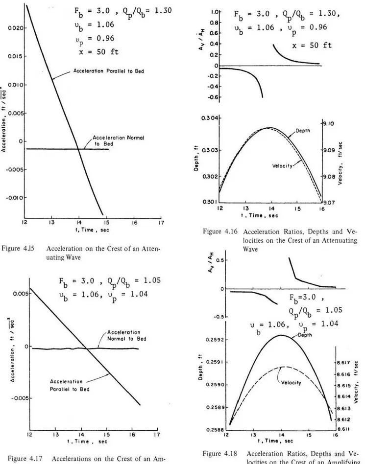
Acceleration on the Crest of an Attenuating Wave

Fb = 3.0 ' Qp/Qb = 1.30 ' Vb = 1.06 ' Vb = 0.96 X= 50ft . . . .

Acceleration Ratios, Depths and Velocities on the Crest of an Attenuating Wave

Fb

=

3.0 ' Op/Qb

=

1.30' Vb

=

1.06 ' Vp = 0.96 X= 50ft . . . .

Accelerations on the Crest of an Amplifying Wave fb

=

3.0 ' Op/Ob

=

1.05 ' Vb = 1.06 ' Vp = 1.04 Acceleration Ratios, Depths and Velocities on the Crest of an Amplifying Wave

Fb

=

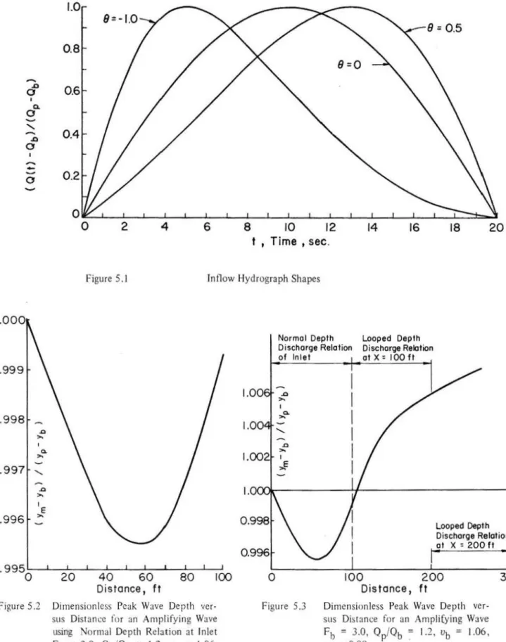
3.0 ' Op/Qb = 1.05 ' Vb = 1.06 ' Vp = 1.04 Inflow Hydrograph Shapes . . . . Dimensionless Peak Wave Depth versus Distance for an Amplifying Wave using Normal Depth Relation at Inlet Fb = 3.0 ' Op/Qb = 1.2 ' Vb = 1.06 ' Vp

=

0.99 1st Order Interpolations . . . . Dimensionless Peak Wave Depth versus Distance for an Amplifying Wave

fb = 3.0 , Qp/Qb = 1.2 , Vb = 1.06 , Vp = 0.99 I st Order Interpolations . . . . .

Discharge Ratio at which Vedernikov Number is One versus Width-Depth Ratio

Fb=3.0 . Yb=0.25 , b=O.O , f=O.Ol . . . .

Dimensionless Peak Wave Depth versus Distance for 20-Second Duration Sinusoidal, lnflo'w Hydrographs of Various Discharge Ratios fb = 3.0 , Vb

=

1.06 . . . .

Dimensionless Peak Wave Depth versus Distance for 20-Second Duration Sinusoidal, Inflow Hydrographs of Various Discharge Ratios Fb

=

3.0 ' Vb

=

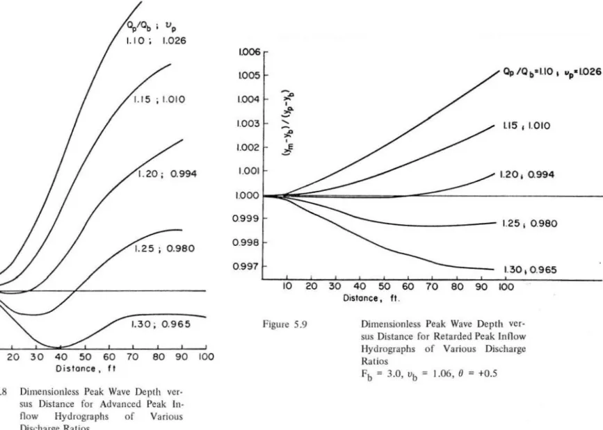
1.06 . . . . Dimensionless Peak Wave Depth versus Distance for a ~Second Duration Sinusoidal, Inflow Hydrographs of Various Discharge Ratios Fb = 3.0 ' Vb = 1.06 . . . . Dimensionless Peak Wave Depth versus Distance for Advanced Peak Inflow Hydrographs of Various Discharge Ratios

fb = 3.0 , Vb = 1.06 , 8 = -1.0 . . . . Dimensionless Peak Wave Depth versus Distance for Retarded Peak Inflow Hydrographs of Various Discharge Ratios

fb=3.0,vb=L06,8=+0.5 . . . . Page 23 23 23 23

25

25 25

27

27

27

27

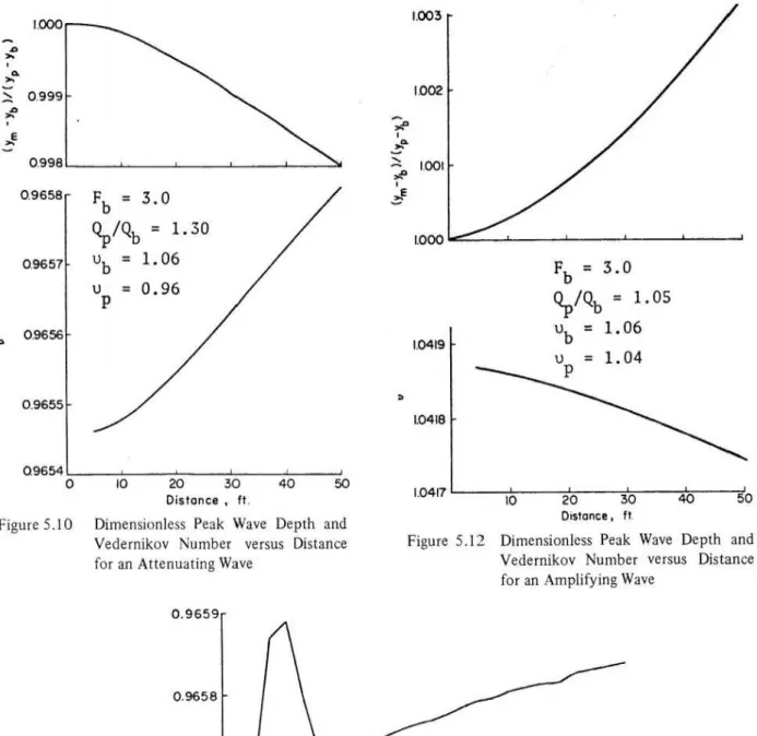
29 29

5.10 5.11 5.12 5.13 5.14 5.15 5.16 5.17 5.18 5.19 5.20 5.21 5.22 5.23 5.24

LIST

OF

FIGURES

(continued

)

Dimensionless Peak Wave Depth and Vedernikov Number versus Distance for an Attenuating Wave

Fb

=

3.0 , Qp/Qb

=

1.30 , Ub

=

1.06 , Up = 0.96

Vedernikov Number versus Distance for an Attenuating Wave Fb = 3.0 ' Qp/Qb = 1.30 , Ub = 1.06 ' Up= 0.96

Dimensionless Peak Wave Depth and Verdernikov Number versus

Distance for an Amplifying Wave

Fb = 3.0 , Op/Qb = 1.05 , Ub = 1.06 , Up= 1.04 Discharge Ratio versus Froude Number of Base Flow B = 1.2 ft, Yb = 0.25 ft , b = 0.0 , f= 0.01 Dimensionless Peak Wave Depth versus Distance for Various Base Flow Froude Numbers

Qp/Ob = 1.3 . . . .

Dimensionless Wave Depth Hydrographs for an Attenuating Wave

Fb

=

1.5 , Qp/Qb = 1.3 , Ub = 0.53 , Up= 0.48 . . . . Dimensionless Wave Depth Hydrographs for a Mildly Attenuating Wave Fb = 3.0 , Op/Qb = 1.3 , Ub = 1.06 • Up= 0.96 . . . .

Dimensionless Wave Depth Hydrographs for an Amplifying Wave

Fb = 4.5 , Qp/Qb = 1.3 , Ub = 1.36 , up= 1.33 . . . .

Dimensionless Wave Depth versus Discharge Plot for an

Attenuating Wave

fb = 1.5 , Qp/Qb = 1.3 , Ub = 0.53 , Up= 0.48 . .

Dimensionless Wave Depth versus Discharge Plot for an Amplifying Wave

Fb = 4.5 , Qp/Qb = 1.3 , Ub = 1.36 ' Up= 1.33 . . Dimensionless Wave Depth versus Discharge Plot for a Mildly Attenuating Wave

Fb = 3.0 , Qp/Qb = 1.30 , Ub = 1.06 , Up= 0.96 Dimensionless Wave Depth versus Discharge Plot for the Crest of a Mildly Attenuating Wave

Fb = 3.0 ' Qp/Qb = I .30 . Ub = 1.06 , Up= 0.96

Velocity Ratio versus Wave Depth for Various Discharge Ratios Fb = 3.0 ' Ub = 1.06 . . . .

Wave Depth where Velocity Ratio is Equal lO One versus Discharge Ratio

Fb = 3.0 . Ub = 1.06 . . . . Dimensionless Wave Depth versus Discharge Plot at the Crest of the Wave for Various Discharge Ratios

Fb = 3.0 , Ub = 1.06 . . . .

Page

30

30 30 31 31 33 33 34 34 34 35 35 35

36

36

LIST OF SYMBOLS

Symbol Definition Symbol Definition

a Coefficient in frictional law R Hydraulic radius- ft

A Cross-sectional area-fe Re Reynolds number- YR/v

AH Acceleration parallel to channel bed-ft/sec2 Sf Frictional slope Ay Acceleration normal to channel bed-ft/sec2 _So Bed slope b Exponential coefficient in frictional law Time- sec

B Base width-ft v Velocity of water particle -ft/sec

c

Chezy resistance constant

v

Average velocity - ft/sec Cs Frictional law constant _Vf Velocity on wave front- ft/sec

c6

Frictional law constant Yo Uniform flow velocity -ft/sec d Cross-sectional shape factor Yr Velocity on wave rear- ft/sec

f Frictional factor X Distance - ft

F Froudc number- Y/.jfy y Depth - ft

Fb Froude number of base flow Yb Base depth -· ft

Fp Froude number of wave peak _Yo Uniform flow depth- ft

Fs Stability Froude number {; + Slope of positive characteristic

g Accelerations due to gravity - 32.2 ft/sec2 € Slope of negative characteristic

k Roughness height _{A Peak parameter of inflow hydrograph}

K

f/8g

8

Skewness parameter of inflow hydrograph

L Reference for integration technique I) Kinematic viscosity m Subscript representing maximum depth at any x p Mass density

p _{Wetted perimeter- ft}

_u

_{Vedernikov number}

q Lateral discharge - ft3 /scc/ft _Ub Ycdernikov number of base flow Q Discharge - fe /sec Up Vedcrnikov number at wave peak

ACKNOWLEDGMENT

This paper is based on the Ph.D. dissertation submitted and defended by J.P. Jolly, and guided and advised by Dr. V. Yevjevich, the major professor and chairman of the Ph.D. committee. Acknowledgment goes also to Dr.

Albert H. Barnes, Associate Professor of Civil Engineering at Colorado State University, for his advice and cooperation, as well as to other members of the Ph.D. committee.

Acknowledgments also go to the U.S. Federal Highway Administration, previously the U.S. Bureau of Public Roads, for their support of the project "Unsteady Free Surface Flow in a Storm Drain," from which some materials have been used, and to the Computer Centre of the University of Ottawa, Ottawa, Canada, where the simulations were made.

The Department of Civil Engineering of the University of Ottawa, Ottawa, Canada, and the Department of

Civil Engineering of Colorado State University, Fort Collins, Colorado, U.S.A., have given all necessary help and encouragement for completion of this study. Both writers gratefully appreciate the support of these institutions.

ABSTRACT

Some hydraulic properties, obtained using the Chezy resistance law, that distinguish amplifying waves from attenuating waves are found by a numerical integration of the governing hyperbolic, partial differential equations of supercritical, gradually varied waves flowing in a channel with a rectangular cross section. The supercritical, gradually varied flow is simulated by using various integration techniques of the specified intervals scheme of the method of characteristics solution to the governing system of equations. One of these integration techniques is

used to determine attenuation and amplification characteristics of gradually varied, single peaked waves. Prior to this determination, criteria found by various investigators for predicting the stability of uniform flow are shown to be equivalent. One of the criteria, the Vedernikov number, which contains parameters dependent on the

frictional law, channel cross-sectional shape and Froude number, is also the criterion for predicting amplification of gradually varied, single peaked waves.

Chapter

1

INTROD

UCT

ION

In most natural and artificially constructed

streams, once a flood wave is in.itiated it will attenuate as it travels along a channel. In some

streams or along spillways, and in many storm

culverts, however, the flow may become supercritical;

and if the Froude number (F : V

f

.JiY)

is above a

.certain value, the peak depth will increase with

distance along the channel. These increases in flow depth can cause excessive hydrodynamic pressures to come to bear against hydraulic structures, as in the

case of a tailrace structure of a hydroelectric station

in the USSR as related by Ghambarian (1965); or

cause the flow to overtop the banks of channels with

steep bed slopes, as is the case of an irrigation canal in

Los Angleles - Brock ( 1967). A criterion or criteria

have not, as yet, been developed to determine

whether or not these supercritical waves will grow in height along a channel.

Instability in open channel flow is defrned as

flow conditions that result when the peak depth of

flow or peak value of any other parameter increases with distance along the channel. In steady flow, the water surface profiJe develops into a series of roll waves that increase in depth at the crests and decrease in depth at the troughs as it travels down the channel.

This is normally referred to as roll waves, and

represents instability of steady flow. With unsteady,

smgle peaked waves instability occurs when the peak

depth of the wave increases with the distance along the channel. This instability has been often observed in nature in open channels (Blair, Cornish, and

Holmes) and normally is referred to as the passage of

gradually varied waves to slug flow.

Unsteady flow may either be gradually varied

or rapidly varied. The equations governing the gradually varied flow are one-dimensional. For this flow it is assumed that the vertical accelerations are small compared with the total accelerations. With

rapidly varied flow the governing equations are

two-dimensional, and the vertical accelerations along

the channel are large when compared with the accelerations parallel to the channel bed.

During the past century, numerous engineers

and mathematicians have developed criteria for deter-mining the stability of open channel flow for a uniform regime but not for unsteady flow. In general,

these criteria give the Froude number above which

3y

3y

(

-

=

0 , -

=

0 ) becomes unstable

3x

3t

uniform flow

for a particular geometry of the cross-sectional area

and the resistance law of flow. These efforts have

been culminated with the work of Vedernikov lwasa Craya, Keulegan and Patterson, each

d

eve

l

o~ing th~

same criterion, but by different methods.

Until 1960 all experiments in open channel flow hydraulics were conducted either in the labora-tory under controlled conditions or in the field. The

types of flow observed were classified as steady or

unsteady and either uniform, gradually varied, or

rapidly varied. Mathematical equations have been

derived to describe these various types of flow - see

bibliography on unsteady flow by Yevjevich (1964).

The solution of these equ,ations represents the flow

that would occur in a physical state_ The available

solutions of these equations, however, were limited to

simplified conditions such as the bed slope and

frictional resistance being equal to zero. Fortunately

during the 1960's methods and techniques became

available for simulating gradually varied flow by the mlmerical integration of the governing equations on a digital computer, thereby providing an alternate to the physical experiments.

In both cases, physical and numerical experiments, there are always errors. In a physical

experiment there are errors resulting from the speci-fication tolerances of the boundary and the initial

conditions and in the means of measuring the flow

parameters. In a numerical experiment, or simulation, although the boundary and initial conditions can be·

prescribed with precision, there still remains both truncation errors in the computations, errors in the

written output, as well as errors resulting from the fmite difference approximations to the mathematical

derivatives and in the integration of the partial

differential equations.

Using the work by Yevjevich and Barnes (1970) and Zovne (1970) on the numerical solution as a point of departure, it .is the objective of this paper to determine the criterion or criteria for instability of gradually varied, single peaked waves. These criteria are determined by numerical simulations, which are

assumed

to be

sufficienlly accurate and far

less

expensi

v

e

to arrive at than from

phy

s

ical

expe

rim

ents.

Moreover

,

it is

questionable

whether

measuring techniques are yet available to accurately

det

erm

in

e,

both

spatially

and

temporally,

the

de

pths

and velocities

s

imultaneously

of

flows

with

high

F

r

oude

numbers.

T

o

descr

ibe these

stabi

lity

phe-nomena

certain

terms have been

used

in the

past.

ln

the work

on

uniform flow

regimes,

the development

of roll waves

has been

referred to as

free

surface

instability (Koloseus and

Davidson)

or

as

instability

(

l

wasa). The

only anal

ytica

l

work so far on the

same

typ

e

of

problem in

supercritical, gradually

varied flow

(Zovnc)

also

uses the terms

stabili

ty and instability.

Both Zovne

and

the writers have used the numerical

sol

utiorr

on

.

the

graduall

y varied flow

equations

in

s

tudying waves

in supercriticaJ regime.

The

solution

of these equations can

be

numerically

unstable under

certai

n

co

nditions

when the flow

is

stable.

Therefore

,

the writers will not use

the

term stability

as use

d

in

the hydraulic

sense

when

discussing gradually varied

flow.

Rather

,

when the peak depths of gradually

varied,

single

peaked waves become smaller as the

waves travel

along

a

channel,

they are said to be

attenuating;

when

the peak depths become

larger

as

the waves travel

along a channel,

they are said to be

amplifying.

When

discussing other

works

with

uniform flow,

h

owever,

the term

stability

will be

used. Therefore, what is being considered

is

the

criterion or cri

teria

for

amp

lifi

cation

of a wave

travelling along a channel

whose

slope

is

supercritical

with

respect to the base f1ow discharge of the

hydrograph.

I

n

other

words, the

amplification of

a

single peaked, supercritical

wave, w

h

ich is

governed

by

the equations of gradually

varied flow, is

studied

with re

spect

to

finding criterion or criter

ia

for

amplification.

Chapter 2

LITERATUR

E

REVIEW

There have been at least three occasions when amplifying waves have been observed in nature and recorded in the literature. Cornish ( 1934) was the fust to mention that the peak depth of supercritical flow in open channels could amplify. By observing the flow in drainage channels in the Swiss Alpes, he noticed that a series of roll waves formed which grew in height as they travelled along a channel.

Two years later Holmes (1936), standing on a bridge over one of the flood control channels in Los Angeles, observed over an interval of several minutes that the flow depth increased from approximately three feet to approximately eight feet and then subsided to three feet. This was followed by another wave of larger amplitude which also subsided to the original flow depth.

Bl~ir

(1961) reported.that on the Nisqually River in the State of Washington in October 1955 that two National Park Rangers observed five or six surges over a duration of 45 minutes which were 15 to 20 feet higher than the water level immediately in front of the surges. The flrst surge washed away a highway bridge that had had 40 feet clearance above

the alluvial bed.

There has been no detailed experimental or theoretical work published that explains why the flow conditions cited above do occur in nature. Moreover, all analytical and experimental studies of amplification in the supercritical regime have been limited to supercritical, uniform flow with the exception of Zovne's work with supercritical, non-uniform flow which will be discussed later.

A review of some of the analytical work on stability criteria for uniform flow is as follows.

Keulegan and Patterson (1940) determined a stability criterion mathematically from Boussinesq's equation for the velocity of propagation of a volume element of a wave and an equation relating frictional resistance with depth for supercritical, uniform flow. They determined that instability will occur when the gravitational force is greater than the frictional force. Their stability criterion is

2 fpV pgyS -o

8

funs table} lstable

J

>

<

0, (2.1)

or in terms of slopes in dividing Equation 2.1 by pgy it can be expressed as

[unstable]

>

0

so -

sf

stable '

<

(2.2)

In Equations 2.1 and

2.2,

p is the fluid density, g is

the acceleration due to gravity, y is the flow depth, S0 is the bed slope, f is the frictional factor, V is the flow velocity' and Sf is the frictional slope.

Also, Vedernikov (1945) determined a stability criterion by using the equations of gradually varied flow and by considering the time growth or decay of energy of a small disturbance on a steady, uniform flow. His criterion is

1 - b dP

u = ( - - ) ( 1 - R - ) F

2

+

b dA

(2.3)

in which

u

is the Vedernikov number, b is the exponential coefficient in the resistance law f= a(Re)b for a hydraulically smooth conduit, R is the hydraulic radius, P is the wetted perimeter, A is the cross-sectional area, F is the Froude number and a is a coefficient. When

u

>

I the flow is unstable; when u=l the flow is neutrally stable; and when

u

<

1 the flow is stable.

Craya (1952) considered steady flow near normal depth thereby eliminating the terms in the gradually varied flow equations that vary with time; thus the partial derivatives become total derivatives. He showed that the flow would become unstable when the Seddon* celerity, dQ/dA , is greater than the Lagrangian celerity, V +

.J'iit ,

i.e.,

dQ/dA

>

V

+

.JiY

(2.4}

Iwasa (1954)' considered the initiation of continuous time growth of an infinitesimally disturbed wave. His criterion for flow with uniform velocity distribution is as follows.

*This celerity is known in the literature under the name Seddon, or Kleitz-Seddon, though the first author to obtain it was Graeff (187 5) before Kleitz (1877) and Seddon ( 1900).

R

dA V

>

dy - ..L-= Fs

< -

-

-

- -

- - - -

-

-(gA

AdR 3

~

j

dA/dy -d-y

c

₂

x 0.4343

c

5

f

+

o.s)

(2.

5

)

in which f is given as 1 f = - -- - -4R ₂

[C5

log

(T

c

₆₎]

k is the height of the resistance roughness, C5 and

c6

are constants.

Iwasa's criterion reduces to Vederni.kov's for compatible conditions.

Koloseus and Davidson (1966), with uniform flows developed in a 3.0 foot wide and 85 foot long flume, obtained good correlation between the sta -bility criterion of Keulegan and Patterson and the development of roll waves. They defjned "roll waves" as any wave of spontaneous origin, regardless of size or shape, that is attributable to no cause other than the superiority of the gravitational force over the boundary retarding force. Although the work by Koloseus and Davidson is interesting but limHed to

depths near normal depth, it is shown in the next chapter that the criteria of Vedernikov, Keulegan and Patterson, and Craya, although expressed in different terms, are equivalent.

One investigator who did not limit his work to super critical, uruform flow was Zovne (

1

970

)

.

Using a digital computer he compared simulated, gradually varied flows. in the supercritical regime with two numerical schemes. He simulated the flows with both the characteristic grid scheme and specified intervals scheme of the method of characteristics and showed that each method gives almost identical results. Both the characteristic grid and specified interval schemes are ways in which the equations of gradually varied flow may be solved by the method of characteristics. He also simu.lated with the specified intervals scheme an experiment in a flume where the raising of a tailgate caused a hydraulic jump to move upstream. In his simulations a sequential depth relation was u'sed, and the wave profiles were not determined at the jump. The experimentally determined and numerically simulated positions of the physical jumps wer.e compared as they moved upstream. Zovne's work provides proof that supercritical, gradually varied flow can be simulated with the method of characteristics. Some of his results are djscussed in Chapter 4.

,·

Chapter

3

THEORETICAL CONSIDERATIONS

3.1

Uniform Flow

In the previous chapter it was stated that the stability criteria developed by Keulegan and

Patter-son, and then by Vedernikov and later bv Crava

are one and the same. To understand this, the work by Keulegan and Patterson should be considered in terms of gravitational and frictional slopes, i.e., instability will occur when S

0

>

Sf

Craya states,

moreover, that instability will occur when the Seddon celerity is greater than the Lagrangian celerity. The Seddon celerity represents the speed of travel of a small wave that has stabilized at an invariant form

and is governed by channel resistance_ The Lagrangian celerity represents the speed of travel of a very small wave under the exclusive actions of inertia and gravity. Since the Seddon celerity is inversely related

to the frictional slope, one may state

that dQ/dA

>

V +

.J"iY

is equivalent

>

<

to

so

<

sf

Consider again the celerity relation for instability dQ/dA

>

V

+

ygy , in a prismatic channel such that y

=

A/B , and A/PR

=

I,

I-b

[ - ]

f

b

V = KR 2

+

b in which K =

8g

and f=a(Re). The Seddon celerity dQ/dA may be expressed as

dV V+A

-dA '

(

3.

1)

and by differentiating the expression for velocity with respect to area

I+ 2b

dV =K(l-b) R 2+b dR

dA (2 +b) dA (3.2)

Now dR/dA may be expressed as

d(A/P) I = -dA P A dP I dP P2 dA =

P

(1 • R dA ) . (3 .3) Therefore dQ I-b A dP - = V + V(- ) - ( 1 - R - ) M ~b PR M (3.4) Equation 3.4 becomes dQ 1 · b dP - =V+V(- )(l·R - ) .

(3.5)

dA 2 + b dA

The criterion for unstable conditions may be expressed by

I· b

dP V(- ) ( I -R - ) 2+ b dA or

v

>

- - - . (3.6)

I

-

b

dP (- ) (I·R - ) 2 + b dA

The left side of Equation 3.6 is by defmition the Froude number, F ; therefore, the criterion may be rewritten in the form

F

=

(3.7)

1 - b dP

(- ) (l·R - )

2+b dA

The Verdernikov number is defined by Equation 2.3, or

1 -b dP

v

= ( - ) ( l · R - ) F 2

+

b dA

which is identical to Equation 3.7, thus the criteria of

slopes - Equation 2.2, Verdernikov number -Equation 2.3, and celerities - Equation 2.4,are one and the same.

3.2

Mathematical Developm

en

t

of

Gradually

Varied Flow Equations

The equations of gradually varied flow, known as the Barre' de Saint-Venant equations, are equa· tions of conservation of mass and conservation of linear momentum or

dV dA dA

A -

+

V -

+

-

•

q = 0 , (3.8)

dx dx dt

dV

dV

dy

pVq

a

v

-

+

~-

+

g -

=

g(S

₀

-Sf)

-A""

,

(3.9)

dx

dt

dx

as

the

conservation of

linear momentum, in

which

I a= - -

I

I

v

3

_dA

AV

3

_A

(3.10)

and

1 ~=-I

I

v2

dA

AV2 A

(3.1

I)

1

n

the

latter two

equations

v

is the

velocity at a

point

in

the

cross

section.

T

hese velocity

coeffic

i

ents,

Equations

3.10 and

3.11,

depend

on

the

velocity

dis

t

ri

bu

tion in a

cross

sec

tional

area of

flow.

l

t is assumed in this

study

that

the velocity distribution is

uni

f

orm; therefore,

a=~ I .

Neither the

lateral inflow nor

outflow

di

scharge,

q

,

are

conside

red

in this

st

udy

.

Be

cause

of the assumed

uniform

veloci

t

y

distribution and

because

lateral inflow

or

outflow are

not

cons

id

ered,

the above equations

sim

plify to

and

dV

dA dA A -

+

V -

+

-

== 0

(3.12)

dx

dx

dt

V

dV

I

dV

-

- +

g

dx

g

dt

dy

+

- =

s . sf

dx

0 (3.

13)

In using

Equations 3.12 and

3.13

to

model

physical flow, the following assumptions are made.

(

1

)

Vertical accelerations a

r

e negligible

.

(2)

The

channel

bed

slope is

mil

d

eno

u

gh

so

that

tana

=

s

ina

.

(3)

Th

e

frictional

slope,

Sf,

ca

n

be

represented by the

Darcy-Wei

s

ba

ch

re

l

a-ti

on

hf=

f

LV

2

_/

_2gd

_R

_{in which f is}

_the

friction factor

as

a

function

of

R

eynolds

number

of

the flow an

d

it is assumed to

be

the same value for

unsteady flow as

for steady

flow, and d is a shape factor.

(

4)

The pressure throughout the flow

d

omai

n

is

hydrostatic.

The third assumption is su fficiem but not

necessary.

Any mathematical

relationship for

fric-tional

slope or any relation

that

equates

it to

a

constant

value will

suffice.

Mor

eo

ver, in this

s

tudy

,.

t

he

Chezy resistance

law

is

used. The

fo

ll

owing shows

the

relationship between

the Chezy

and

Da

r

cy-Weisba

c

h

relati

ons.

The Chezy

resistance Jaw

relates

fl

ow velocity

to hydraulic radius and the f

r

ictional slo

p

e.

I

t

may

be

stated

as

V

=

C

vRSf

in which

C

is

the Chezy

constant.

The Dar

cy-

Wei

s

bach

resistance states

that

Sf=

f

V

2

/2gd

R in

which d is a constant

that

is

dependent

only

on

the

cross-sectio

n

al

shape

.

For

circ

ular

sections

d is

equal

to

four,

and

for

very wide

rectangular

cross sections

d is equa

l

to one.

Ot

her

cross-sectiona

l

shapes

have intermediate values

of

d .

The

frictional factor,

f, is relate

d

to

R

eyno

l

ds

number

by

f =

a(Re)b

in whkh Re

= Vyfv ,

in

which

v is kinematic viscosi

t

y. Thus, the

Darcy-W

eisbach relation may be

written as

a y2

+

b

s f =

-2g

dvbRl-b

and the

Ch~zy

relation as

The

two relations

are the same when

b

=

0

and

C

=

J2gdv/a ,

which is a

constan

t f

or

given

con

di

-tions

o

f

fluid, temperature, cross-sectional shape and

r

o

ughne

ss.

The

eq

u

ations

of

unsteady

free-surface

flow,

Equations

3.

1

2

and

3.13

,

form a system of

quasi-linear, partial hyperbo

l

ic differen

t

ia

l

eq

u

ations of the

first order.

Vari

o

u

s

possib

l

e

methods

for integrating

these

two

partia

l

diffe

r

entia

l

e

q

ua

t

ions

ar

e revie

w

ed

in ref

e

rence

s

abstracted by Yevjev

.

ich

(1964). One

of

th

ese

methods is the method of cha

r

acter

i

stics which

was

s

hown

by Zovne

(

1

970)

to be applicable

for

s

upercriti

ca

l

flow.

J

t was developed by

M

assau (1889)

f

o

r integrating th

e

two

partial

differentia

l

equations

of

un

s

t

eady

fl

o

w in

channe

l

s

by

a graphical

pr

ocedu

r

e·.

T

h

is

method

ha

s

been

a

l

so

widely used f

o

r

the

so

luti

on of a

variety

of

p

roblems

in phy

sics an

d

mechani

cs,

and

its

detaile

d

description

can

be

found

in Courant and Freidrichs (I

948

)

,

Crandall

(19

56

)

,

and Streeter a

n

d W

ylie

( 196

7).

Th

e solut

i

on of

a

specific

problem by

the

method

of cha

ra

cteris

ti

cs

using hand calculation,

o

r

graphica

l

means,

o

r

desk

calc

ulat

o

r

s

is

extreme

ly

laborious and time

consum

in

g.

A

s

a result in the

interval

between

1

889

and

the

advent of electronic

co

mputer

s,

a variety

of sc

h

e

me

s

for solving open

c

hann

e

l

flow problems by this

method was

proposed. The details of these various schemes can be found in references abstracted by Yevjevich

(1964).

In general, solutions by the method of characteristics may be performed in two ways:· by the graphical

method and by the use of digital computers. Of the

two, digital computer provides several advantages. A digital computer can not only do the tedious com

-putations that are required for the graphical method, but it can also give the solution for the complete system of equations to a better degree of accuracy

and precision.

In both procedures the method of

characteris-tics uses the equations of continuity and momentum of unsteady t1ow,

(3.12)

and

(3.1

3

)

,

along with the total differentials of the dependent variables, velocity and depth, which constitute four characteristic

equations. By considering only prismatic channels

-those of unvarying cross-sectional areas and constant

bed slopes - then the cross-sectional area may be described by A = By where y is the hydraulic depth. Thus, the characteristic equations are

and A av ay 1 ay

- -

+

-

+

- -= VB ax ax V at

v

av

- -

+

g

ax av

- +

g

at av dV=rx dx+dt ay dt, ay ay dy = - · dx + - dt ax at

0

_,

(3.14)

(3.16)

(3

.

17)

The partial derivatives of y and V with respect to x and t are unknown, therefore, there are four equations and four unknowns. A method is now described that shows how the four equations are solved simultaneously for V and y at any x and t . The four equations can be expressed in the matrix equation: A 1 av

VJJ

0

v

Ox

0

v

I av 0

_Ot

=

_So-sf g g ay (3.18) dx dt 0 0

_Ox

dV 0 0 dx dt

_Ot

ay dy

This equation may be expressed in the format of matrix algebra as: [M] x [Z] = [N) , in which

[M] is the coefficient matrix, and [Z] and [N]

are vectors representing the unknown partial derivatives and the right side of the equation,

respectively.

To obtain a solution of V and y at any x

and t from this equation, let t.M be the determinant of a matrix [M) and

let AK.i represent a matrix formed by replacing a

column (i) in [M) by [N) . From matrix algebra it

may be proved that Zi

=

.6K/ t.M . The rows of [M] are linearly dependent, i.e., there is an interdependency between the values of y and the

values of V at any x and t.To satisfy this

interdependency the determinant of the coefficient

rna trix t.M must be equal to zero. Here the

equation [M] [Z] =

[N

]

becomes indeterminate

av av ay ay and the values of - - - and - are

ax 'at . ax at not uniquely determined, i.e., zi

=

AK/t.M =

0

/

0.

Therefore, since the derivative must be finite in the flow phenomenon considered, t.Ki must equal zero

whenever .6M equals zero.

By expanding the determinant of [M) and equating it to zero, a quadratic equation in dt/dx is

obtained. Solving for both positive and negative

values of dt/dx the following is obtained

dt

<crx}

=

- -

-

--v+VAiJB

(3.19)

and dt

(QX")

-

,

= V- JAg/B e_ •

(3

.20

)

The curves in the distance-time plane on which .6M = 0 are called the characteristics curves. On each, the value of dt/dx is a constant.

By expanding the determinant of any of the

four t.Ki in Equation 3.18 and setting it equal to

zero, four different but equivalent partial differential

equations are obtained of the type shown in the following equation.

{ A V d t I } dy A dV

[

- -

-

]

-

+

-

-

+ --

+

VB g dx g dx VBg dx A dt

W

(So· Sf)-

co.

dx (3.21)

SubstJtuting the values of e±from Equation 3.19 and 3.20 to· Equation 3.21 the following ordinary differential equations in V and y are obtained:

{ A V

1J

dy A dV

[ - -

-

]e

.+

- -

+

- -

+

VB g g dx V Bg dx (3.22)

[

[

~-~]e.~}

dy

+~

dV

+

~

VB

g

g

dx

VBg

dx A

"VB

(S₀ . Sf) e_

=

o,

(3.23)

along the positive and negative characteristics, respectively.

To numerically integrate the above equations in order to determine the depth, y , and velocity, V , at any distance, x , and time, t , in a channel there are many schemes. Two of them are described in the next chapter. To reiterate both are schemes of a class of solution known as the method of characteristics. One is called the characteristic grid scheme; the other

,.

C

h

a

pter

4

N

UM

E

RI

CAL S

OL

UTI

O

NS O

F

G

R

A

DUALL

Y

VARI

E

D FL

O

W

EQUAT

IONS

4

.1 Intr

o

du

ct

ion

In part 3~2 of Chapter

3,

in which the

mathematical equations of gradually varied flow were

discussed in terms of the characteristic equations,

both the characteristic grid and the specified intervals

schemes of integrating the equations were mentioned.

There are many other methods available by which

these equations can be integrated, such as the

Lax-Wendoff and the diffusing schemes. A survey of

the available methods with a discussion of their

advantages and limitations for the numerical integra·

tions of the gradually varied flow equations may be

found in a recent publication by Yevjevich and

Barnes (

1970).

These investigators recommended the

use of the method of characteristic over any other

method. The two schemes of the method of

characteristics are described in the following

para-graphs.

4

.

2 Characte

risiti

c G

rid

Sc

h

e

m

e

The pair of first-order equations that represent

the flow, Equations

3.22

and

3

.23,

of the previous

chapter, have two real roots,

_(OX).=

dt _E+ and

dt

<ax)

_

=

e_. A curve that at each of its points has dt

the slope

<ax)+

is called a positive characteristic. A curve that at each of its points it.tS the slope

dt

(CIX)_

is :ailed a negative characteristic. There

are, therefore, two families of intersecting curves that

fill out the domain of the independent variables x

and t . Typical patterns of intersecting characteris·

tics for subcritical and supercritical flows are shown

in Figure 4.1.

By a simultaneous solution of Equations 3.19,

3.20, 3.22,

and

3.23,

the depths and velocities of the flow may be determined at the points where the

positive and negative characteristics intersect. They

are found by integrating from two grid points where

y and V are known, points R and S , to the third

point, P which is the intersection of the characteris

-tics that pass through points R and S shown

schematically in Figure 4.2. To obtain y and V at

point P after knowing their values at points R and

S the equations resulting from the simultaneous

solutions of Equations

3.19,

3.20,

3.22

and

3.23

are solved in a sequential order. These equations are:

xs-xR + tR(VR+

v'iY'R).

ts(V s. -hYs>

tp= (4.1)

(4.2)

(4.3)

By means of the above equations y and V

can be determined at any point on the (x,t)-plane by

changing the grid size or shape by varying .:lt and .:lx.

4.3 S

pe

ci

fi

e

d In

terv

als

Sc

h

e

m

e

One way to describe the specified intervals

scheme for integrating the equations of gradually

varied flow is to consider the (x, t)- plane subdivided

into grids of equal sized rectangles, each .:lx long

and .:lt high. The initial conditions V and y arc

known along the lower boundary corresponding to

t = 0 and the upstream conditions are known along

the left boundary of Figure 4.3.

Assuming that y and V are known at every

grid point along the line t = 11 • tlt as shown in

Figure 4.3, then y and V can be determined at the

grid points along t

=

t1 in the following manner.

Consider that y and V are to be determined at

point P . By determining the slopes of the

charac-teristics that pass through point P , the positions

where the characteristics cross the line t1 -.:lt (points

R and S) can be found. The values of depths and

velocities at these points can then be calculated by

(a) Subcriticol Flow F < I

£t=--==-Vt../9Y

I

E =

-V-../QY

(b) Supercriticol Flow I

€-

•

-F

>I

Fi

g

ure

4.1

b

Fi

gure

4.2

V-ffy"

Families

of

Characteristic Curves

for

both Subcritical

and

Supercrit

i

ca

1

Flows

Grid

for the Solution

by

Chara

cte

r-istic

Grid

Scheme

X

neighbourhood of points R and S . From these values the frictional slopes and the coefficients in Equations 3.22 and 3.23 can be evaluated, and the

equations can be integrated along the characteristics

to determine y and V at point P .

Equations 3.22 and 3.23 may be expressed in the following algebraic form proceeding from points

R and S on the t1 -At )jne to the point P on the t1 line, as

(FJR(Yp·YR) + (GJR(VP-VR)

+

(SJR (xp-xR) = 0 , (4.5) along the positive characteristic, and as

(FJs(Yp·Ys)

+

(GJs(Vp-V s)

+

(SJs(Xp·xs) = 0,

(4.6) along the negative characteristic. In these equations the coefficients have

{,A

V

I

}

(FJs =

l

[vs

.

g-

1

e_

+g-

s , A (GJR

=

(VBg )R ' A (GJs =

Cvsg

)

s

,

and

Using the values of V and y at points R and

S , Equations 4.5 and 4.6 are solved simultaneously to determine the depth and velocity at the point

P, i.

e., [(T.)R (G.)R] (TJs (G)s (4.7)

Dp

=

[

(F j R _(G.)R] (FJs (G_)s and [ (F.)R

(

T

.)

Rl

(F Js CTJs

v

---p -[(F.)R (G.)R] (F Js (GJs (4.8) in which (TJ R = (F.)R · YR

+

(G.)R VR · (S.)R (xp-xR), and (T Js = (F Js Ys + (GJs V S. (SJs(Xp·Xs) .

The solution is continued in the x direction ftrst and then continued for successive values of t , at At intervals apart, until the flow in the channel is

simulated for a specified duration.

4.4 Co

mp

ariso

n

s

of So

lu

t

i

ons

Ob

ta

in

e

d

b

y

th

e

Charact

er

i

s

tic Grid and

Specifie

d

Interv

al

s

Sc

h

e

m

es

Some of the disadvantages in using the

cha.racteristjc grid scheme are as follows.

1. The depths and velocities are obtained on the (x,t)-pJane in an uneven distribution of grid points. To obtain results in an orderly distribution, interpolations for calculated depths and velocities must be carried out in the x and t directions. Any

order of interpolation possesses certain numerical errors that undermine some of the precision of the

characterisitc grid scheme.

2. It is difficult to space the characteristics of the same sign a suitable distance apart along the x and t axes. For example, the flow regimes in regions I and 3 in Figure 4.1 are independent of each other, and the flows in region 2 are dependent on conditions

in region 1 and 3; therefore, it is impossible to know the spatial intervals of the characteristics in region 2

beforehand.

3. Members of the same family of character

is-tics in the supercritical regi.me may converge with flows of high Froude number. When this occurs, the depth and velocity at the grid point are no longer

In contrast to the problem associated with the

characteristic grid scheme, the specified intervals

scheme has certain advantages. One of them is that

the grid spacing is known beforehand. The numerical

solution is also more systematic, and the depths and

velocities can be obtained at grid points where

adjacent characteristics converge, which is precluded

in the characteristic grid scheme.

Some of the work by Zovne can be used to

infer other advantages in using the specified intervals

scheme. He considered hypotheticaJ, supercritical

flow in which a linearly decreasing hydrograph was

simulated by both the characteristic grid and the

specified intervals schemes. His results are shown in Figure 4.4. It can be seen that the solutions from the

two schemes are almost identical which, in view of

the difficulties of the characteristic grid scheme

described above, lends support to the use of specified

intervals scheme for simulating supercritical flows in

this and similar studies.

Some of the assumptions necessary for using

the specified intervals scheme are as follows.

I. Interpolation must be used to determine the

depths and velocities at the points where the charac·

teristics that pass through point P cross the line

t J ·bot, (points R and S).

2. It is assumed that the slopes of the charac·

teristics at point P are the same as at point C . In

other words, it is assumed the change in slopes of the

characteristics over a bot time interval is small; if this

assumption can not be madeJan iterative scheme must

be used to re-evaluate the slopes of the characterlstic

equations and in turn the values of the coefficients in

Equations 4.5 and 4.6.

3. It is assumed that the curvature of the

characteristics over bot interval is negligible. AI·

though the errors associated with the assumptions in

[1) and [2) can be reduced by the refinement of the

algorithm, there is no way, as yet, to reduce this error

as an operating program.

4. The grid size of the specified intervals scheme must be smaller than with the characteristic

grid scheme for the same degree of accuracy, since

both the positive and negative characteristics that

pass through point P must cross within a grid

spacing in order fur the interpolation equations to be

valid. This condition of both positive and negative

characteristics passing through a single grid spacing is

sometimes referred to as the Courant condition for

numerical stability, which states that bot= box/01

+

vgy).

Although this numerical stability criterion

was first used by Massau with his work on the

graphicaJ solution of the differential equations of

unsteady flow, it has been referred to as the Courant

stability criterion by recent researchers such as

Liggett and Woolhiser (1967), Streeter and Wylie

(1967), and Zovne (1970). To avoid confusion in the

literature, the writers will also refer to this stability

criterion as the Courant condition.

The specified intervals scheme is used to

determine the criterion for amplification in this

study. Some of the limitations with regard to

accuracy of the scheme as described in the four

assumptions discussed above will be discussed in more

detail in the next section.

4

.

5 Ac

c

ur

acy

of

Specified I

n

t

e

rv

a

l

s

Sc

h

e

m

e

in

S

imulatin

g S

up

ercr

iti

c

al Fl

o

w

s

4.5 .I Introduction. It has been demonstrated by

Pinkayan and Barnes (1967) that the smaller the Ax

size in the specified intervals scheme, and thus the

smaJ!er the bot used in order to satisfy the Courant

condition, the more accurately the scheme will

compare with observed flows in the subcritical

regime. In the supercriticaJ regime, however, there arc

few observed flows with which comparisons can be

made.

Zovne, in his comparisons of characteristics

grid and specified intervals schemes, assumed that the

slopes of the characteristics changed a negligible

amount over the At interval at any grid point along

the channel. He used two point interpolations to

determine the positions (points R and S) in Figure 4.3 where the characteristics cross the line t 1· bot

from the values of the dependent variables at the grid

points and he evaluated the values of the coefficients

of Equations 4.5 and 4.6 at points R and S,

respectively. The comparison of results obtained from the specified intervals scheme with the results

obtained from the characteristic grid scheme shows

good correlation as shown in Figure 4.4. Zovne also

stated that the use of a second order interpolation

equations and the averages of the values of frictional

slopes between points P and R and between

points P and S improved the accuracy of the

scheme, although their usc was not warranted in his

0.5

0.4

:o

.3

-

c s:; 0. ~0.2

t

A Figure 4.3 Figure 4.4

p

7.1

fi.T

8

R

s c

l\X

Grid for lhe Solution by Specified Intervals Scheme

D

B

=

3.5 ft

E

X

Specified Intervals Scheme DX=20ft

x

=

I 000 ft o Characteristic Grid Scheme DX=20ft t:. Characteristic Grid Scheme DX= I 0 ft Initio I Froude Number I. 748 Fino I Froude Number I. 52

2

)(

=

2000 ft 0 TIme in seconds

Comparison of Solution by Character-istic Grid and Specified Intervals

A term-integration technique - that has not

appeared as yet in the literature pertaining to the

specified intervals scheme - will be used throughout

the remainder of the text. This technique is as follows. Interpolation equations of various order are used to determine values of the dependent variables at points R and S after the positions on the t 1 -tt.t line of the latter are found from the slopes of the

characteristics. Then the coefficients of Equations 4.5

and 4.6 are evaluated at either point C or at points

R and S. Once the equations have been integrated, the slopes of characteristics of point P may or may

not be redetermined and the above procedure is

repeated until two successive values of characteristic

slopes are within a specified tolerance. The technique

from determining where the characteristics cross the

t ]-tt.t line to finding the values of the dependent

variable, with or without iterations, at point P will be called an integration technique. Moreover, an integration technique that includes a particular order

of interpolation equations to determine the values of

the dependent variables at points R and S is prefixed with the order of the interpolations. Therefore, a technique that uses third order

interpolation equations is called a third order

integration technique.

In this study, where the flow conditions at

which a wave neither amplifies nor attenuates are to be determined, the most accurate technique possible must be used. The tests conducted to determine the refinements to the basic first order integration

technique to obtain the most accurate algorithm were

simulated in a rectangular shaped channel, the sides

of which are hydraulically smooth. A constant base

flow governed by the Chezy resistance relation is

introduced into this channel. The inlet conditions are

sinusoidal hydrographs superimposed on the base

flow. The depth-discharge relation at the inlet (rating

curve) is the normal depth relation.

The refinements that are made to the specified

intervals scheme to improve its accuracy arc: (a)

decreasing the grid size; (b) increasing the order of

the interpolation equations used to determine the

values of the dependent variables at points R and

S ; (c) evaluating the coefficients of Equations 4.5

and 4.6 at points R and S instead of at point C ,

where most of the current investigators have

evalu-ated them - Henderson (1966), Streeter and Wylie

(1967), and Yevjevich and Barnes (1970); (d) once

the depth and velocity have been calculated at point

P using the characteristic slopes at point C ; then

the characteristic slopes are re-evaluated at point P ,

and new depth and velocity determined at point P .

This is continued by using an iterative procedure until

successive values of calculated characteristic slopes

are within a particular tolerance. The tolerance used

for this study was 0.00001 feet.

The last refinements, (b), (c), and (d) are

discussed under the subject of integration techniques.

The effects of the first refinement is as follows.

4.5.2 Grid size. Once the tt.x size has been chosen then the At size is specified by the Courant stability

condition. Therefore, by varying the Ax the size of

the grid mesh is also varied. Considering a wave flowing on a base flow of high Froude number such that the wave should amplify throughout the length of the channel, then the grid size should be small

enough so that the simulated wave does amplify

throughout the length of the challliel.

Figure 4.5 shows the results of a wave resulting

from a sinusojdaJ inflow hydrograph of 20 seconds

duration with a discharge ratio, Qp/Qb == 1.05 flowing in a rectangular channel 1.2 feet wide on a

base flow with a depth of 0.25 feet and a Froude

number of 3.0. This figure shows the dimensionless peak wave depth at 40 feet from the inlet versus the

tt.x used in the integration.

The specifications of the integration technique are such that the slopes of the characteristics at point

P are the same as at point C ; first order inte

rpola-tions are used to determine the values of dependent variables at points R and S, and the coefficients of

Equations 4.5 and 4.6 were evaluated at points C .

It may be seen that when Ax is larger than two, the wave peak depth at 40 feet from the inlet is less than the peak depth at the inlet. When the Ax is less than two feet, the peak wave depth at 40 feet are larger than at the inlet. Since the discharge ratio is

small and the base flow width-depth ratio is

large, B/Y b == 4.8 , then by the theory of small

disturbance on uniform flow, the peak depth should increase as the wave travels along the channel

(Koloseus and Davidian). Therefore, for the inflow

conditions tested a tt.x smaller than two feet should

be used. It may be seen also from Figure 4.5 that when tt.x is decreased from two feet to one foot, there is a very small increase in wave depth at 40 feet. This may be better seen in Figure 4.6 where the peak

Q.

"'

1.01 :::: 0.99 0.97 0_·96_{o~----~2~---4+----*6---~a~----~~o~----~~2~----~~~4-----7.1G} Ax , fl Figure 4.5 1.02 1.0 I

Effect of Grid Size on Peak Depths

Fb = 3.0, Qp/Qb = 1.05, ub

=

1.06

up = 1.04

lst Order Interpolations x = 40 ft

~ Ax= 2.5 ft·Gregory- Newton

'

~

0.99

Ax

=

5 ft- Gregory· Newton 0.98~~---L--~~~~5~0~~--L-~--~~10~0---­ Distonce , ft

Figure 4.6 Effect of Grid Size on Peak Depths Fb = 3.0, Qp/Qb = 1.05,

ub

= 1.06 up= 1.04