Lund 2010-02-16
Department of Industrial management & Logistics production management
Analysis of a coordinated
multi-echelon inventory control
system
-A case study on its performance compared to the
current inventory control system at
A master thesis project
Supervisor:
Peter Berling
Authors:
Oskar Callenås Christian Lindén
I
Preface
This master thesis was performed during a time period of 20 weeks from September 2009 until January 2010. The project corresponds to 30 ECT and it is the final part of the Master of Science program Industrial Engineering and Management at Lund Institute of Technology, Lund University. The study was executed at Syncron in cooperation with the division of Production Management at Lund Institute of Technology.
The master thesis was performed with the knowledge that we have learned during our four years of studding at Lund University and the goal has always been that both Syncron and the University will benefit from the results.
There are several people who have made this master thesis possible. First we would like to thank our supervisors at Syncron, Cecilia Wiman and Daniel Martinsson. We also would like to give great thanks to Sara Östborg, who has answered our questions well about the SCP. At Lund Institute of Technology we would like to thank our supervisor Peter Berling for all the time he has invested in this project. We also would like to thank Johan Marklund who has helped us with the analytical model during his paternity leave. Finally we would like to thank everybody at Syncron in Malmö, where the major part of the work has been done. Lund, januari 2010
Oskar Callenås Christian Lindén
III
Abstract
Even though the coordinated inventory control is becoming more well-known, it is relative unused by companies, whose advantages of using it should be obvious. This master thesis illustrates the result of using coordinated inventory control compared to a currently used non-coordinated inventory control.
There exist precise coordinated methods for control of a multi-echelon inventory system, but they are too computationally complex to use in practice. Approximations are needed to allow a coordinated inventory control in practice and not just in theory. The basic idea with the coordinated model evaluated in this master thesis is to introduce an induced backorder cost at the central warehouse allowing decompose of the multi-echelon inventory system to several single-echelon inventory systems. The inventory system which the model decomposes is a distribution system with one central warehouse and N different retailers. The coordinated model has earlier been used and tested in real case scenarios and other master thesis, but since then it has been developed to improve its performance.
The study began by selecting a number of articles that represent the actual material flow within the studied inventory system. Then the reorder points of all the selected articles were calculated with the coordinated model. The calculated reorder points were then compared, by simulations in the simulation software Extend, with the current reorder points obtained from Syncron. The reorder points from Syncron are calculated without any coordinated inventory control. The results of the project have shown that by using a coordinated inventory control of the inventory system, the total inventory in the system is reduced significantly, with about 35%, while the service level most of the times is improved or at least maintained. Most of the inventory within the inventory system has shifted from the central warehouse out to the retailers.
V
Sammanfattning
Vid lagerstyrning av ett flernivålagersystem används idag för det mesta inte en koordinerad lagerstyrning. Trots att den koordinerade lagerstyrningen börjar bli mer utbredd så är den relativ oanvänd ute hos företagen, vars nytta av att använda den skulle vara påtaglig. Detta examensarbete visar på resultatet av att använda en koordinerad lagerstyrning jämfört med en icke koordinerad lagerstyrning.
Det finns exakta koordinerade metoder för styrning av flernivålagersystem men de är för beräkningstunga för att kunna användas i praktiken. Genom att ta fram och använda sig av approximationer kan den teoretiska koordinerad lagerstyrning användas praktiskt. Grundtanken med den koordinerade modellen som analyseras i detta examensarbete är att införa en fiktiv bristkostnad som möjliggör nedbrytning av ett flernivålagersystem till flera enkla lagersystem. Lagersystemet som bryts ned består av ett centrallager och N stycken olika återförsäljare. Den koordinerade modellen har använts och testats tidigare på flera verkliga scenarier och i andra examensarbete, men sedan dess har modellen utvecklats för att förbättra dess resultat.
Studien startade med att välja ut ett antal artiklar som representerar det verkliga flödet av material i det studerade lagersystemet. Därefter beräknades beställningspunkter fram för alla valda artiklar med hjälp av modellen för koordinerad lagerstyrning. De beräknade beställningspunkterna jämfördes därefter med de nuvarande beställningspunkterna från Syncron, som är framtagna utan koordinerad lagerstyrning, i simuleringsmjukvaran Extend
Resultaten från studien visar att användandet av en koordinerad styrning av ett lagersystem kan reduceras det totala lagret i systemet kraftigt, med i genomsnitt 35 %, samtidigt som servicenivån i systemet i de flesta fall förbättras eller i alla fall bibehålls. Den stora skillnaden som sker inom lagersystemet är att lagernivån sänks hos centrallagret och istället förskjuts ut till de olika återförsäljarna.
VI
VII
Table of figures
Figure 1 – Syncrons solutions (Manage your global supply chain easily - Syncron-,
2009) ... 2
Figure 2 – Report outline ... 5
Figure 3 – Density and cumulative distribution function for a normal distribution (Wikipedia, den fria encyklopedin, 2009) ... 17
Figure 4 - Density and cumulative distribution function for an exponential distribution (Wikipedia, den fria encyklopedin, 2009) ... 18
Figure 5 - Density and cumulative distribution function for a gamma distribution (Wikipedia, den fria encyklopedin, 2009) ... 21
Figure 6 – A single-echelon inventory system ... 22
Figure 7 - (R, Q)-policy with continues review and continuous demand. ... 22
Figure 8 – A multi-echelon distribution system ... 27
Figure 9 – The undershoot problem with non-continuous demand. ... 34
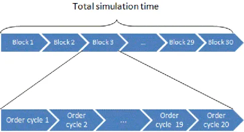
Figure 10 – Overview on the simulation time setup. The total simulation time consist of 30 blocks. One block consist of 20 order cycles and one order cycle is at least 500 time units long, often longer. ... 48
Figure 11 – Difference from target fillrate, normal distributed settings as customer demand ... 57
Figure 12 – Spread from target fillrate, normal distributed settings as customer demand ... 58
Figure 13 – Difference from target fillrate, compound Poisson settings as customer demand ... 60
Figure 14 - Difference from target fillrate, compound Poisson settings as customer demand, fast articles ... 62
Figure 15 - Difference from target fillrate, compound Poisson settings as customer demand, slow articles ... 63
Figure 16 - Difference from target fillrate, compound Poisson settings as customer demand, lumpy articles ... 65
Figure 17 - Difference from target fillrate, compound Poisson settings as customer demand, demand < 20 ... 66
Figure 18 - Difference from target fillrate, compound Poisson settings as customer demand, 20 < demand < 100 ... 67
Figure 19 - Difference from target fillrate, compound Poisson settings as customer demand, 100 < demand < 1000 ... 68
Figure 20 - Difference from target fillrate, compound Poisson settings as customer demand, 1000 < demand < 5000 ... 69
VIII
Figure 21 - Difference from target fillrate, Negative Binominal settings as customer
demand ... 70
Figure 22 – Inventory reduction for Group 1 ... 72
Figure 23 – Inventory reduction, example article ... 73
Figure 24 – Inventory reduction, fast articles within Group 2 ... 75
Figure 25 - Inventory reduction, slow articles within Group 2 ... 75
IX
Frame of tables
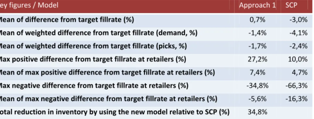
Table 1 – Key figures ... 51
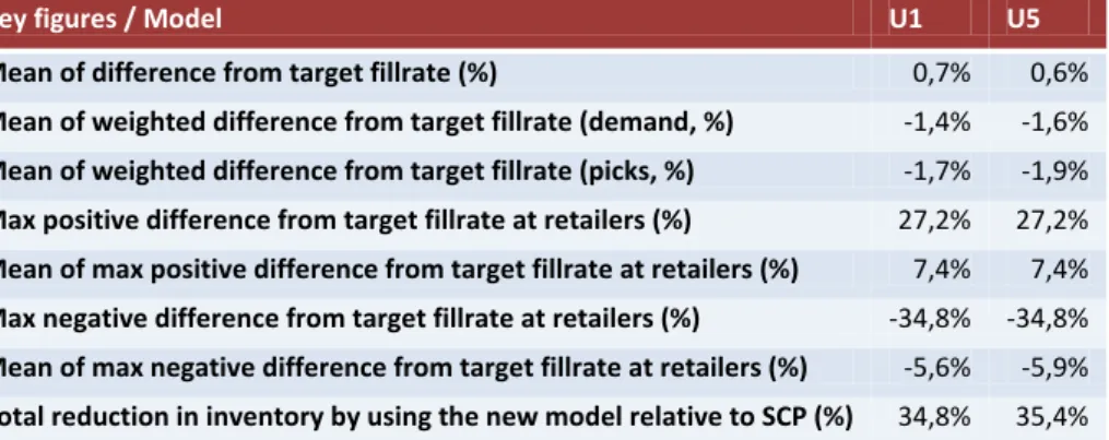
Table 2 – Key figures, choose of undershoot method 1 or 5 ... 55
Table 3 – Key figures, normal distributed settings as customer demand ... 56
Table 4 – Key figures, compound Poisson settings as customer demand ... 58
Table 5 - Key figures, compound Poisson settings as customer demand, fast articles ... 61
Table 6 - Key figures, compound Poisson settings as customer demand, slow articles ... 62
Table 7 - Key figures, compound Poisson settings as customer demand, lumpy articles ... 64
Table 8 - Key figures, Negative Binominal settings as customer demand ... 70
Table 9 - Key figures, Problem articles ... 71
Table 10 – Key figures, example article ... 73
Table 11 – reorder points, example article ... 74
XI
Table of contents
Preface
... I
Abstract
... III
Sammanfattning
... V
Table of figures
... VII
Frame of tables
... IX
1
Introduction
... 1
1.1 Syncron ... 1 1.2 Problem background ... 3 1.3 Problem definition ... 4 1.4 Objective ... 4 1.5 Purpose ... 4 1.6 Delimitations ... 4 1.7 Target Group ... 4 1.8 Report outline ... 52
Methodology
... 7
2.1 Scientific approach ... 72.1.1 Scientific approach used in this project ... 7
2.2 Data gathering ... 7
2.2.1 Literature review ... 7
2.2.2 Data gathered by others ... 8
2.2.3 Data gathering used in this project ... 8
2.3 Methods of analysis ... 9
2.3.1 Method of analysis used in this project ... 10
2.4 Credibility ... 10
2.4.1 Validity ... 10
2.4.2 Reliability ... 11
2.4.3 Objectivity ... 11
2.4.4 Credibility in this project ... 11
2.5 Approach depending on knowledge ... 12
2.5.1 Approach depending on knowledge used in this project ... 13
XII
2.6.1 Practical approach used in this project ... 14
3
Theoretical framework
... 15
3.1 General definitions ... 15 3.2 Statistical distributions ... 16 3.2.1 Normal distribution ... 16 3.2.2 Exponential distribution ... 18 3.2.3 Poisson distribution... 193.2.4 Compound Poisson distribution ... 19
3.2.5 Gamma distribution ... 20
3.3 Single-echelon inventory systems ... 21
3.3.1 Optimization of a reorder point in a single-echelon inventory system 23 3.4 Multi-echelon inventory systems ... 26
3.4.1 Determine a reorder point in multi-echelon inventory systems .... 27
3.5 Model for heuristic coordination of a decentralized inventory system 28 3.5.1 Optimizing of the reorder points ... 30
3.6 “Under-shoot”-adjustment ... 33
4
Data processing
... 37
4.1 Received data ... 37
4.2 Sorting ... 37
4.3 Current reorder points ... 40
5
Calculation of reorder points
... 41
5.1 Input data ... 41
5.2 Settings ... 42
5.3 Calculations depending on undershoot and demand ... 44
6
Simulations
... 45
6.1 The simulation model ... 45
6.1.1 Assumptions made in the simulation ... 46
6.1.2 Verification of the simulation model ... 46
6.1.3 Runtime of the simulations ... 47
6.2 Input parameters ... 48
6.3 Output parameters ... 49
7
Results and analysis
... 51
7.1 Key figures and grouping ... 51
XIII
7.1.2 Grouping ... 53
7.2 Choose of undershoot method ... 54
7.3 Different demand approaches compared to the SCP ... 55
7.3.1 Normal distribution settings as customer demand ... 56
7.3.2 Compound Poisson settings as customer demand ... 58
7.3.3 Negative Binominal setting and problem articles ... 69
7.4 Inventory allocation ... 71
8
Conclusions and discussion
... 77
8.1 Discussion ... 78
8.1.1 Holding costs and shortage costs ... 78
8.1.2 The reality differ ... 79
8.1.3 Implementation... 79
8.2 Future research ... 80
9
Source reference
... 81
Appendix 1 - Pivot table
... 83
Appendix 2 - Interface of the Excel-model
... 84
Appendix 3 - Extend model: overview
... 85
Appendix 4 - Extend model: part 1
... 87
Appendix 5 - Extend model: part 2
... 88
Appendix 6 - Extend model: part 3
... 89
Appendix 7 - Extend model: part 4
... 90
Appendix 8 - Extend model: customer demand generator block and
retailer trigger block
... 91
Appendix 9 - Extend model: retailer inventory block
... 92
Appendix 10 - Extend model: central warehouse block
... 93
Appendix 11 - Extend model: splitter block
... 94
Appendix 12 - Extend model: cost calculation block
... 95
Appendix 13 - Extend model: indata and outdata
... 96
1
1 Introduction
In this chapter the company Syncron is described. The problem background
and problem definition, delimitations, objective, purpose, target group and
report outline are discussed.
1.1 Syncron
Syncron is a global company with offices in the most of the world such as Japan, United Kingdom, Australia, India, Italy and Sweden. They deliver software and services for global supply chain planning, fulfillment and supply. The company has been in the supply chain business for over 15 years and Syncron has delivered significant results for industry leaders such as Volvo, Tetra Pak and Astra Zeneca (Manage your global supply chain easily - Syncron-, 2009).
Syncron has developed core values that influence the whole company. Whatever they do the core values have been chosen to help them do it the right way. The core values are (Manage your global supply chain easily - Syncron-, 2009):
• Customer success, Syncron is developing the best solution for the customer, in order to create a maximum value.
• Always ahead, the customer will gain access to thought leadership that will help them to stay ahead of competition.
• Global perspective, no matter where the customer is located, Syncron is there for them.
• Make a difference, Syncron takes pride in their work and strive to always exceed expectations.
• Fairness and respect, Syncron treat each other with respect and maintain fairness in all relationships.
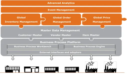
Syncron has five solutions they sell to their customers. The solutions easily enable global processes across the extended supply chain whilst leveraging the customers’ existing investment in ERP systems (Manage your global supply chain easily - Syncron-, 2009). The solutions can be overviewed in Figure 1 below:
2
Figure 1 – Syncrons solutions (Manage your global supply chain easily - Syncron-, 2009)
Business Process Platform
Syncrons Business Process Platform (BPP) is based on Service Oriented Architecture (SOA) which means that the platform is able to adapt after its customers processes. All Syncrons solutions are built on the BPP. Hence, everyone that implements someone of Syncrons solutions needs the BPP. The platform consists of three major parts (Manage your global supply chain easily - Syncron-, 2009):
• Business process workbench, which is used to design the services and process in what is called Workflows and Micro flows.
• Business process engine, which is responsible for executing the Workflows and Micro flows.
• External interfaces and adaptors.
Master data management
In many companies their data is stored in different databases that sometimes are spread all over the world. This makes it hard to reach the data and sometimes the data could disappear, which can affect and reduce the operational efficiency. Syncron Master Data Management (MDM) brings together all the dispersed master data into one master store, available from everywhere (Manage your global supply chain easily - Syncron-, 2009).
3
Global inventory management
The Global Inventory Management (GIM) optimizing the customers global inventories and ensures that the right goods are always at the right place at the right time and in the right quantity. Through an interface that is simple to use, large number of products in a complex global chain is made easy to manage (Manage your global supply chain easily - Syncron-, 2009).
Global order management
The Global Order Management (GOM) manages the customers global order fulfillment with a single process. It integrates the internal and external business systems so Syncrons customers can provide their customers with real time information, which enable for an example track and trace information (Manage your global supply chain easily - Syncron-, 2009).
Global price management:
With increasing globalization it is important to be able to adjust prices to stay competitive. The Global Price Management (GPM) supports the different steps in a pricing process from data gathering to price setting and execution. It helps the customer to quickly analyze and synchronize new prices across the organization, with significantly reduced administrative costs (Manage your global supply chain easily - Syncron-, 2009).
1.2 Problem background
Today, there is no effective and simple method to optimize the reorder points in a multi-echelon inventory system. Syncron is currently controlling the ordering process (i.e. the reorder points) in a decentralized manner without any direct coordination between the different echelons. The division of Production Management at Lund University has developed a procedure for calculating the reorder points in a similar manner but with a great potential for improved coordination. This is done with the introduction of an induced backorder cost at the central warehouse, allowing the multi-echelon inventory system to be broken down into several single-echelon inventory systems. The coordinated model has earlier been used and tested in real case scenarios and other master thesis, the problem then was that the service level was not achieved. But since then the model has been developed to improve its performance, this has yet to be verified and tested though.
4
1.3 Problem definition
This master thesis evaluates the model originally developed at the division of Production Management at Lund University. The following issue should be answered:
• What is the potential of this new coordinated model compared with the current uncoordinated method used by Syncron?
1.4 Objective
The objective is to evaluate a specific model, developed at the division of Production Management at Lund University, for the control of a multi-echelon inventory system. Furthermore, the reduction of inventory level will be analyzed, with the simulation software Extend, when a coordinated method is used instead of an uncoordinated method. The project also evaluates how well the model fulfills the service levels defined by Syncron.
1.5 Purpose
The purpose is to carry out the evaluation in a proper and independent point of view, and to create a report where the potential and the underlying theory of the model are described. The purpose is also that the outcome will be of value for both the University and Syncron.
1.6 Delimitations
The study includes a multi-echelon inventory system with a central warehouse linked to the maximum of 11 retailers. All the demand data in the multi-echelon inventory system is taken from one of Syncron customers and all the data is limited over the time period of one year. All the demand data comes from a multi-echelon inventory system that handles spare parts. The study includes 135 articles that have been restricted down from about 39,000 articles. There is no direct demand from the central warehouse, all the demand goes through the retailers.
1.7 Target Group
The target groups of this master thesis are primarily Syncron, the division of Production Management at Lund University and other NGIL partners. Also students, especially those studying inventory management are the target group.
5
1.8 Report outline
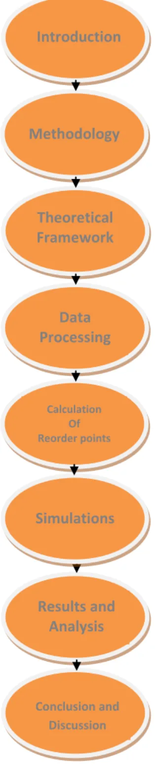
The report is divided into following chapters:
Chapter 1 – Introduction
The first chapter provides a description of Syncron, it also provides a description of the problem and the objective with this master thesis.
Chapter 2 – Methodology
The second chapter presents the methodology, which this master thesis is based on.
Chapter 3 – Theoretical framework
In this chapter the theoretical framework needed to understand this master thesis is presented to the reader.
Chapter 4 – Data processing
In this chapter the data obtained from Syncron and how the chosen articles were selected is presented.
Chapter 5 – Calculation of reorder points
This chapter describes how reorder points is calculated with the analytical model, programmed in Excel and Visual Basics.
Chapter 6 – Simulations
This chapter contains a brief description of the simulation model structure and the assumptions made, as well as input and output parameters.
Chapter 7 – Results and analysis
In this chapter the results from the simulations are presented and analyzed.
Chapter 8 – Conclusion and discussion
This chapter contains the conclusion of the results and a discussion around some different aspects and assumptions that might affect the results of the simulations.
Figure 2 – Report outline
Introduction Methodology Theoretical Framework Data Processing Calculation Of Reorder points Results and Analysis Conclusion and Discussion Simulations
7
2 Methodology
In this chapter the methodology which this master thesis is based on is
presented. First the general methodology in the form of scientific approach,
data gathering, method of analysis and credibility is presented, followed by
approach depending on knowledge and our practical approach.
2.1 Scientific approach
During a paper, there are two main directions of approach that should be chosen between, inductive and deductive. The inductive approach starts with the empirical and based on that, models and theories are created. The deductive approach begins with the theory and an empirical study is carried out so that the theory is tested. An approach going back and forth between the two above-mentioned theories is called abduction (Björklund & Paulsson, 2003, p. 62), (Wallén, 1996, p. 47).
2.1.1 Scientific approach used in this project
In this master thesis a deductive approach was used. First, the theory of multi-echelon inventory systems and specific models were understood and described, and then data was collected and simulated to evaluate the model.
2.2 Data gathering
The purpose of the study determine when choosing a method to collect data. There are two different methods to choose from, quantitative and qualitative data collection method. All information in quantitative studies can be measured or evaluated numerically while qualitative studies aims at providing a comprehensive picture of the situation. Mathematical models are usually suitable for quantitative studies and interviews are often useful for qualitative studies (Björklund & Paulsson, 2003, p. 63).
Depending on what kind of information that is collected, data can be divided into two different groups, primary data and secondary data. Primary data is collected to be used in the current study and secondary data is data collected for a purpose other than the current study (Björklund & Paulsson, 2003, pp. 67-68).
2.2.1 Literature review
Examples of literary studies are magazines, books and newspapers. Any form of written material is literature and the literature is mostly secondary data. When the literature is used in a study, it is important to remain critical because it is easy
8
to manipulate the texts and it is not always that the text is comprehensive. Some positive things about literature are that much information can be addressed quickly, it is usually easy to access and it can be accessed with small economic resources (Björklund & Paulsson, 2003, pp. 67,69).
2.2.2 Data gathered by others
Sometimes it's very difficult to get hold of data and sometimes it is impossible because the authority to collect it is denied. Then it is appropriate to use data that others have collected. By using data gathered by others the investigation time can be reduced. There are generally four different types of data collected by others (Höst, Regnell, & Runeson, 2006, p. 98):
• Processed material: Data collected by others and processed for an example in academic publications and theses.
• Available statistics: Data collected and processed without any conclusions. For an example, data from Statistics Sweden.
• Index data: Data collected for any purpose and is available in unprocessed form. For an example data in a customer database.
• Archive Data: Data that is not systemized. For an example, protocol.
2.2.3 Data gathering used in this project
In the beginning of this master thesis data was collected directly from Syncron. All this data can be measured or evaluated numerically, which makes it quantitative. This data was not created for this master thesis, which makes it secondary data. During the process of the work a lot of data came as output from the simulations. This data is also quantitative; it can be measured or evaluated numerically. This is new data and it was the key to answer the problem definition, which makes it primary data.
Literature review
Literature studies are the basis for any theory used in the thesis. Sources were carefully analyzed to be sure that no false information was used and that the authors understood the problem.
Data gathered by others
Since this master thesis builds on real customer demand data received from a third company, all data used came from Syncron and was stored in their SCP software. This means that all data is index data which is not processed in any way.
9
Criticism to gathered data
The data gained from Syncron and their SCP software is as previously said secondary information and its accuracy cannot be verified by the authors. But since it is index data it is assumed to be correct and that no modifications have been done with it. One problem encountered during the thesis work was that the obtained data from Syncron could distinguish because of different settings in the SCP software. An example of the settings was if trends were allowed. However after tests with different setting in the SCP and checks and comparisons with own calculations, all data is seen as correct. Syncron helped out a lot with the tests with different settings in the SCP, though it is also in Syncrons interest that the study is carried out on the correct data so that they can benefit from the outcome.
All literature used in the project is considered to have high credibility. Articles are taken from respected international journals where the research work are refereed and must be of a high standard to be published. The books and internet sources used is believed to be accurate because the authors possess the knowledge to determine this, which they can do because of their knowledge from their education.
2.3 Methods of analysis
Data can be analyzed in several different ways to answer the purpose of the project. Several methods of data analysis are available and what/which to use depends primarily on the nature of the data collected; if it is quantitative or qualitative (Höst, Regnell, & Runeson, 2006, p. 110). Since the data used in this master thesis is only quantitative, only those three methods are described in more detail.
The analysis of quantitative data includes the following three different methods; use of analytical models, statistical processing and modeling/simulation. Analytical models are used to structure and evaluate the collected data. The models can be either strictly adhere to the theory or be specifically customized for the analyzed situation. By statistical processing of the data collected, new information can be obtained from the current data such as mean and standard deviation of the data. A correlation analysis can also be carried out between different variables which can indicate strength in the relationship between variables. This processing can be done manually, but mostly some form of computer software specifically adapted
10
for this purpose is used. With the help of simulation tools different scenarios are tested and the results compared (Björklund & Paulsson, 2003, pp. 71-73).
2.3.1 Method of analysis used in this project
To answer the purpose of this master thesis a couple of analyzes have been made off the collected data. First a huge amount of simulations where done to be able to have some output data to which statistical data processing was used. Microsoft Excel was an important tool used to retrieve, for example mean and standard deviation on the data which was the foundation for the upcoming data sorting process. From the statistical processing of the output, key figures were obtained and used in the comparison between the different methods evaluated in this project.
2.4 Credibility
When simulation models are used to evaluate different methods peer performance, it is required that the model and its results are "correct". A high level of credibility of the research project is obtained when three different aspects are met: validity, reliability and objectivity (Björklund & Paulsson, 2003, p. 59).
2.4.1 Validity
Validity is defined as “to what extent something really measures what it intends to measure" (Björklund & Paulsson, 2003, p. 59). A model may have validity for an experiment, but not for another, i.e. a model is developed specifically for one purpose, and the validity is determined from this. For the validation of a simulation model there are four general angles, performing self-validation, validation is performed by the model user, a third party performing the validation, validation is performed using a scoring model (Sargent, 2004).
The most common way to perform validation is that the developers do it themselves. This is a subjective decision based on the results of a number of tests carried out during the model development process. However, credibility will be suffering in this approach because the developer's objectivity is questionable. To increase the objectivity and for the most part, the number of persons performing the validation of the model, the users can carry out the validation. Even in this case, however, objectivity can be questioned. By allowing an independent third party to perform validation, commonly known as "independent verification and validation (IV&V), an objective validation is obtained. This adds credibility and is often used when large costs are associated with the development of the model. When IV & V is used, it is most straightforward to only evaluate the validation that
11
has already been done. Finally, a scoring model can be used. This method is rarely used in practice (Sargent, 2004).
Which focus the validation has depends on the model's character. When the model's underlying theories and assumptions has to be assured a conceptual validation is carried out. It also decides if the model is consistent with its purpose. Computerized model validation is used when it should be ensured that the programming and implementation of the model is correct. Operational validation aims to establish that the model’s output is sufficiently consistent with why the model was created (Sargent, 2004).
2.4.2 Reliability
That different measurement, of the same kind and on the same objects, produces the same result is called reliability. This means that the measurements do not contain random errors and that the instrument is reliable. Comparing the differences between the maximum and minimum value can assess reliability of a series of measurements and a reliability coefficient can be obtained by calculating the correlation between two different measurement series (Wallén, 1996, p. 67).
2.4.3 Objectivity
Objectivity is the extent to which values influence the study. The objectivity may be increased if the reader all the time gets all reasoning clearly explained to them and thus take its own position on the outcome. By reproduce sources properly and avoid distortion of the underlying facts as the example to use value-charged words, objectivity is further increased (Björklund & Paulsson, 2003, pp. 61-62).
2.4.4 Credibility in this project
The authors have made all their decisions and assumptions in this project with a continuous target of maintaining the credibility.
Validity
In this master thesis, its developers and its users make the validation of the models. The focus will be on computer-based and operational validation. Since this project is based on quantitative data, i.e. measurable numbers, there is no scope for measurement error. All models have therefore been validated by at least one of the first two of Sargents angles for the validation of a simulation model. In those cases where assumptions were made that could affect or even reduce the validity, it has been carefully commented upon in the report.
12
The analytical model is created and tested by researchers in the area and it is therefore considered to be very valid. In cases where inconsistencies have emerged that the authors could not explain, they were shown for the creators who subsequently have been able to find the problem area. The simulation model used in this project is an expansion of an existing and well-tested model. In order to assure that the results of the new simulation model is correct; the results from a number of test simulations were compared with the existing model. When the same input resulted in the same output in both models, the expanded simulation model is considered to have a high validity.
Reliability
By conducting several experiments in a steady state procedure in the simulations, the reliability is achieved in this master thesis. Since simulations are based on historical data from a limited period of time, it is a great possibility that the input data used may change if a similar study is carried out in the future. A change in demand, lead time or fillrate over time is highly likely which in this case might affect the results a bit. That the results will differ markedly, however, is not likely as the result of this report is based on a variety of demand patterns, lead times, fillrates, etc. Therefore it is not considered that a change in the parameters affect the reliability.
Objectivity
The authors tried much as possible to let their own values stand aside. All tests were carried out with a neutral approach and all choices were reasoned well. It is therefore considered that report have a high level of objectivity.
2.5 Approach depending on knowledge
What level of ambition a research project has depends largely on the level of knowledge held within the area. The literature distinguishes between four different studies, exploratory study, descriptive study, explanatory study and normative study, which in turn lead to the study carried out in various ways (Wallén, 1996, p. 46).
When the study aims to obtain basic knowledge about the problem and its nature, an exploratory study is carried out. As an example, typical cases and variables are specified, and concepts that are relevant to the problem are determined. A project that aims to determine the characteristics of the research project uses a so-called descriptive study. Here, data is collected and systematized in order to determine values of the variables and their interaction. An explanatory study is
13
used when the scope of the project is to "explain". Cause-effect and systemic effects are some of the explanations that may be relevant to illuminate. Finally described are normative studies, where the results of the study will provide a norm- or action proposal. In these studies often value issues, ethical issues and political issues comes in. Their disagreement is here presented as well as various proposals for action and its impact on the various parties involved (Wallén, 1996, pp. 46-47).
2.5.1 Approach depending on knowledge used in this project
In this master thesis, the approach based on the level of knowledge has been as an explanatory study. The various methods for calculating the reorder point is evaluated against each other and why difference in outcome occurs is described.
2.6 Practical approach
The approach of this master thesis can be defined with an operations research. An operations research can be divided into six stages (Hillier & Lieberman, 2005, p. 8):
1. Defining the problem and collect relevant data
2. Create a mathematical model representing the problem
3. Develop a methodology to develop a solution to the problem of model 4. Test the model and improve it
5. Prepare to implement the model 6. Implementation
In the first step the problem area is studied and based on that study a problem is defined. Once that's done, it is important to involve all partners and make them understand that the problem exists and that it needed to be resolved. After that, data is collected to create an overall picture of the problem. Another reason for collecting data is to ensure that raw data is available to put into the model created in step two (Hillier & Lieberman, 2005, pp. 8-11).
In the second step a mathematical model based on the significantly of the problem is created. Here it is important to start with a simple version and then improve it gradually to finally have a model that represents this problem well (Hillier & Lieberman, 2005, pp. 12-14).
In the third step a method (often computer-based) is created to develop a solution that represents the problem in the model. It's easy to believe that this step is what takes most time, but this is often not the case. Already developed
14
programs, for an example Excel and Visual Basics, which easily can model the problem, is often used here (Hillier & Lieberman, 2005, pp. 15-17).
In the fourth step, the model is tested and improved. Almost always when big mathematical models have been built bugs occurs that need to be resolved. The more accurate the model is tested and the more bugs that are eliminated, the greater the validity of the model will be. The model can be tested in different ways, for an example it can be tested, like in this case, with a simulation program. (Hillier & Lieberman, 2005, pp. 17-19).
In the fifth step a well-documented system is created to prepare for implementation of the model. The system will contain the model, solution method of the model and worked procedures for implementation. Often, this is a computerized system that needs a number of computer programs to work (Hillier & Lieberman, 2005, pp. 19-20).
In the sixth step, the system is implemented. Here it is important that the team who worked on the model is participating because they know the model best. During implementation, it is important to constantly provide feedback how implementation is progressing. If major differences arise from the tests, a decision must be taken about changing the model (Hillier & Lieberman, 2005, p. 21).
2.6.1 Practical approach used in this project
This master thesis follows the work procedure of an operations research project described above. The first step, the problem definition, was at first established among all those involved in the project so that everybody understood which data was relevant to have in order to solve the problem. Then data was received, sorted and fitted to the prebuilt analytical model. Most of the work in this master thesis has been devoted to the 4th step where the analytical model has been
validated and tested in conjunction to an existing inventory control model (Syncrons current model) with the simulation program Extend. The result of step five, which is this report, evaluates the two inventory control models against each other and offer advice for future implementations. The sixth step falls outside the scope of this master thesis and is therefore delimitated.
Some of the steps where already done by others or existing software could be used and therefore a limited amount of time in this project has been put on these steps. E.g. step two and three where the analytical model was developed and programmed at the division of Production Management at Lund University.
15
3 Theoretical framework
In this chapter the theoretical framework for the master thesis is presented.
The theoretical framework is important for the understanding of the project.
First some general definitions are presented, followed by theory of
statistical distributions and different inventory systems. The main thing
described in the theoretical framework is decompose of a multi-echelon
inventory system in to several single echelon inventory systems by
introducing an induced shortage cost.
3.1 General definitions
Holding costs: By having stock, capital is tied-up. These costs are primarily capital costs and the cost of warehouse buildings, insurance, and rejects are included here (Axsäter, 1991, p. 39).
Setup costs: When an order shall be produced, setup costs arise. This depends on setup costs and running cost for different machines (Axsäter, 1991, p. 39).
Ordering costs: For new orders, administrative costs of purchase and shipping and handling costs arise. Ordering costs and shortage costs are balanced against holding costs to determine Q (order quantity) (Axsäter, 1991, p. 39).
Shortage costs: These costs are costs that arise when one cannot deliver directly when one unit is demanded. It is very difficult to assess the costs as they are difficult to measure. These costs are balanced against holding costs to determine R (reorder point) (Axsäter, 1991, p. 39).
Lead time: The time from order to delivery and it includes possible delays e.g. due to stockouts at previous echelons (Axsäter, 1991, p. 13).
Service level: When shortages costs are difficult to measure a different concept has developed; service requirements. Three common definitions of service requirement are defined below (SERV1, SERV2 and SERV3). In this master thesis SERV2
16
and SERV3 is used. (Axsäter, 1991, p. 40). More definitions
exist.
SERV1: Probability of no stock out during an order cycle
(Axsäter, 1991, p. 68).
SERV2: Fraction of demand that can be satisfied immediately from
stock on hand, also known as fillrate (Axsäter, 1991, p. 68). SERV3: Fraction of time with positive stock on hand, also known as
ready rate (Axsäter, 2006, p. 94).
Backorder: Units that have been demanded but not yet delivered
(Axsäter, 2006, p. 46).
Inventory position: Stock on hand + outstanding orders - backorders (Axsäter, 2006, p. 46).
3.2 Statistical distributions
Customer demand is normally uncertain but it still has to be described in some manner. A common way of doing so is to use statistical distribution functions. This section describes the distribution functions used in this master thesis to describe the customer demand when reorder points are calculated, see chapter 5 for a description of how the calculation is done.
3.2.1 Normal distribution
A normal distribution, also called Gauss distribution, is a continuous distribution with a density function that can be described as a bell-shaped curve that is symmetric around μ, see Figure 3 (Vännman, 2002, pp. 115-116), (Ross, 1985, p. 34).
17
Figure 3 – Density and cumulative distribution function for a normal distribution (Wikipedia, den fria encyklopedin, 2009)
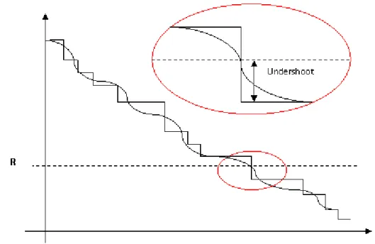
The normal distribution is perhaps the best known of all continuous distributions and it is suitable to use as a stochastic model if phenomenon that can be understood as the sum of many random variables are studied (Vännman, 2002, pp. 115, 165). The central limit theorem says that under very general conditions, a sum of many independent random variables will have a distribution that is approximately normal. In many situations, the demand comes from many independent customers, and their demand can then be represented by a normal distribution (Axsäter, 2006, p. 85). One problem that might arise when a continuous distribution is used as an approximation of the reality is the undershoot problem described in section 3.4.4.
The normal distribution is suitable to use as an approximation when the demand is high, but not when the demand is low. A good rule to follow is that the ration between the mean and the standard deviation shall be above two (Berling & Marklund, 2009). The reason for not using the normal distribution when demand is low is the high probability of negative demand (Axsäter, 1991, pp. 66-67). In such situation the demand is better approximated using other distribution functions e.g. Poisson distribution (described in section 3.2.3) or Compound Poisson distribution (described in section 3.2.4). The normal distributions density function and cumulative distribution function describes as follows (Vännman, 2002, p. 155):
Density function:
𝜑𝜑(𝑥𝑥) = 1 𝜎𝜎√2𝜋𝜋𝑒𝑒
18 Cumulative distribution function:
𝜙𝜙(𝑡𝑡) = 𝑓𝑓(𝑡𝑡)𝑑𝑑𝑡𝑡 (3.2)
The parameters μ and σ is the expected value and the standard deviation of demand (Vännman, 2002, p. 155).
3.2.2 Exponential distribution
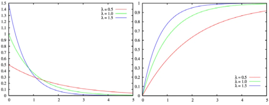
An exponential distribution is a continuous distribution with a density function that can be described as a ski slope; see Figure 4 below (Vännman, 2002, p. 113).
Figure 4 - Density and cumulative distribution function for an exponential distribution (Wikipedia, den fria encyklopedin, 2009)
Time between events that occur randomly and are independent of each other is often exponential distributed (Vännman, 2002, p. 113). An example is time between customer arrivals. They occur randomly and often independently of each other. The exponential distributions density function and cumulative distribution function describes as follows (Ross, 1985, p. 33), (Vännman, 2002, p. 113): Density function:
𝜑𝜑(𝑥𝑥) = �𝜆𝜆𝑒𝑒−𝜆𝜆𝑥𝑥, 𝑥𝑥 ≤ 0
0, 𝑥𝑥 > 0 (3.3)
Cumulative distribution function:
𝜙𝜙(𝑥𝑥) = �0, 𝑥𝑥 ≤ 0
1 − 𝑒𝑒−𝜆𝜆𝑥𝑥 𝑥𝑥 > 0 (3.4)
The parameter λ is the number of arrivals over a period of time, and 1/ λ is the arrival intensity.
19
3.2.3 Poisson distribution
A Poisson distribution is a discrete distribution. The distribution can be described as a series of events that occur randomly and independently of each other during a time interval (Vännman, 2002, p. 85). When time between customer arrivals are exponential distributed and the customers only demands one unit at the time the demand follows a Poisson process (Law & Kelton, 2000, pp. 325-326). The Poisson distribution is easy to handle and it is appropriate to use when the demand is relative low. An example of low frequency demand is spare parts (Axsäter, 1991, p. 146), like in the studied inventory system in this master thesis.
The number of independent Poisson distributed customer arrivals, where each customer demands one unit, over a period of time t, can be described as follows (Axsäter, 2006, p. 78):
𝑃𝑃(𝑘𝑘) = 𝜆𝜆𝑡𝑡𝑘𝑘! 𝑒𝑒𝑘𝑘 −𝜆𝜆𝜆𝜆, 𝑘𝑘 = 0,1,2 … (3.5) The parameter λ indicates the average number of events during time period t (Vännman, 2002, p. 85).
It's very convenient and computationally efficient to use a Poisson distribution. But it is important that the variance (σ2) divided by the mean (μ) is approximately
equal to one. A good rule that can be used to determine whether a Poisson distribution fits the demand process is 0.9 ≤ (𝜎𝜎2)/𝜇𝜇 ≤ 1.1 (Axsäter, 2006, p. 85).
3.2.4 Compound Poisson distribution
During a Poisson distributed demand, each customer only request one unit. While for a compound Poisson distributed demand, each customer can request one or several units at the time. This is the big difference between the Poisson distribution and the compound Poisson distribution. The distribution of demand size in the compound Poisson distribution is stochastic and is called the compounding distribution (Axsäter, 2006, pp. 78-79).
𝑓𝑓𝑗𝑗𝑘𝑘: Probability that k customers give the total demand j D(t): Stochastic demand in the time interval t.
𝑃𝑃(𝐷𝐷(𝑡𝑡) = 𝑗𝑗) = �𝜆𝜆𝑡𝑡𝑘𝑘! 𝑒𝑒𝑘𝑘 −𝜆𝜆𝑡𝑡𝑓𝑓 𝑗𝑗𝑘𝑘 ∞
𝑘𝑘=0
20
The variance (σ2) divided by the mean (µ) must be > 1 to use a compound Poisson
distribution and the compound Poisson distribution is appropriate to use when the relation above is (σ2/µ) > 1.1 (Axsäter, 2006, p. 78).
If the studied event is customer arrivals, then the time between customer arrivals is defined as 1/λ where λ is calculated through the following expression (Axsäter, 2006, p. 79):
µ: average demand per unit of time fj: probability of demand size j (j = 1,2, … ).
𝜇𝜇 = 𝜆𝜆 � 𝑗𝑗𝑓𝑓𝑗𝑗 ∞ 𝑗𝑗 =1 ↔ 𝜆𝜆 =∑ 𝜇𝜇𝑗𝑗𝑓𝑓 𝑗𝑗 ∞ 𝑗𝑗 =1 (3.7)
When a Compound Poisson distribution is fitted to the demand, the compounding distribution can be very complex and computational complex. If that is the case, it is easy to fit a predefined distribution to the compounding distribution. When a logarithmic compounding distribution is fitted to the compound Poisson distribution the distribution is called a negative binominal distribution (Axsäter, 2006, p. 78). This is the compounding distribution used to approximate customer demand in the SCP software and for computationally complex articles in the analytical model.
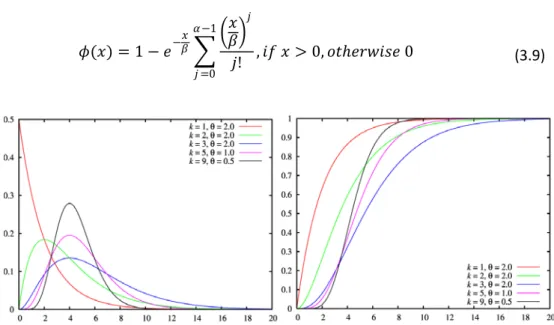
3.2.5 Gamma distribution
A gamma distribution is a continuous distribution. The distribution has two input parameters, a shape parameter (α) and a scale parameter (β). If the shape parameter (α) = 1 the gamma distribution is the same as an exponential distribution. The exponential distributions density function and cumulative distribution function describes as follows (Law & Kelton, 2000, pp. 301-303): Density function:
21 Cumulative distribution function:
𝜙𝜙(𝑥𝑥) = 1 − 𝑒𝑒−𝑥𝑥𝛽𝛽 ��𝑥𝑥𝛽𝛽� 𝑗𝑗 𝑗𝑗! , 𝑖𝑖𝑓𝑓 𝑥𝑥 > 0, 𝑜𝑜𝑡𝑡ℎ𝑒𝑒𝑒𝑒𝑒𝑒𝑖𝑖𝑒𝑒𝑒𝑒 0 𝛼𝛼−1 𝑗𝑗 =0 (3.9)
Figure 5 - Density and cumulative distribution function for a gamma distribution (Wikipedia, den fria encyklopedin, 2009)
If the variance (σ2) divided by the mean (µ) is < 1, but not too far from one, there
is a risk for negative demand when using a normal distribution (see section 3.2.1). The normal distribution is often a good alternative even though the variance (σ2)
divided by the mean (µ) is close to one, but an alternative in these cases is to use a gamma distribution where the demand always is nonnegative (Axsäter, 2006, p. 86).
3.3 Single-echelon inventory systems
An inventory system considered as a single-echelon inventory system is characterized by two properties (Axsäter, 1991, p. 38):
• Different types of articles should be controlled independently.
• Articles are kept in stock only in a single-echelon inventory system, not in multi-echelon inventory system.
22
Figure 6 – A single-echelon inventory system
Traders are examples where single-echelon inventory systems are used. They often sell products from a single output stock and can then manage their warehouse through a single-echelon inventory system. Various cost parameters that are optimized and considered in a single-echelon inventory system are (Axsäter, 1991, pp. 38-39):
• Holding costs
• Ordering costs and Setup costs • Shortage costs or Service level
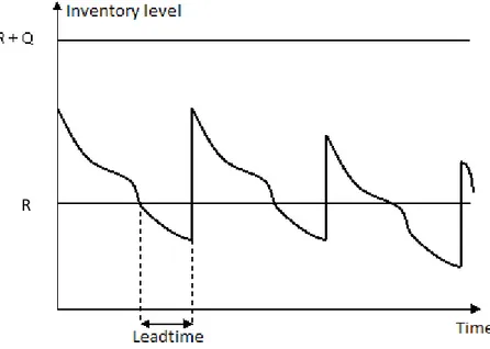
A common reordering point system for single-echelon inventory system is called an (R, Q)-policy. When the stock position is equal to or less than the reorder point (R), the order quantity (Q) is ordered. The review and the demand can be booth periodic and continuous, se Figure 7 for a (R, Q)-policy with continues review and a continuous demand. (Axsäter, 1991, p. 42).
Figure 7 - (R, Q)-policy with continues review and continuous demand.
23
3.3.1 Optimization of a reorder point in a single-echelon inventory system
There are many ways to optimize reorder points in a single-echelon inventory system. For example it could depend upon if the demand is relative low or high, if cost optimization or fillrate optimization is used (Axsäter, 2006, pp. 77, 94). Two methods used within this master thesis are optimization against holding and backorder cost and meeting a fillrate constraint, which are described below. To optimize a single-echelon inventory system with a normal or a compound Poisson distributed demand, a (R,Q)-policy with a given batch quantity Q, constant lead times, continuous inspection and a backorder system the following notations is needed (Axsäter, 2006, p. 91).
Q: order quantity
R: reorder point
h: holding cost per unit and time unit p: shortage cost per unit and time unit µ’: mean of lead-time demand
σ’: standard deviation of lead-time demand φ(): distribution function of the normal distribution ϕ(x): density function of the normal distribution
fk: probability for demand size k for the compounding distribution
k: positive demand size j: positive inventory level
Normal distribution
First the fillrate optimizing procedure is described. For a normal distributed demand the distribution function of the inventory level is (Axsäter, 2006, p. 91):
𝐹𝐹(𝑥𝑥) = 𝑃𝑃(𝐼𝐼𝐼𝐼 ≤ 𝑥𝑥) =𝑄𝑄1�𝑅𝑅+𝑄𝑄�1 − 𝜙𝜙(𝑢𝑢 − 𝑥𝑥 − 𝜇𝜇𝜎𝜎′ ′)� 𝑑𝑑𝑢𝑢
𝑅𝑅 (3.10)
The lost cost function, which is a function that measures the degree of wrongness, i.e. the difference between estimated and the true value, is defined as (Axsäter, 2006, p. 91):
𝐺𝐺(𝑥𝑥) = 𝜑𝜑(𝑥𝑥) − 𝑥𝑥(1 − Φ(𝑥𝑥)) (3.11) and
24
𝐺𝐺′(𝑥𝑥) = Φ(𝑥𝑥) − 1 (3.12)
Using (3.12), (3.10) can be reformulated as (Axsäter, 2006, p. 92):
F(x) =𝑄𝑄1� �−𝐺𝐺′�𝑢𝑢 − 𝑥𝑥 − 𝜇𝜇′ 𝜎𝜎′ �� 𝑑𝑑𝑢𝑢 𝑅𝑅+𝑄𝑄 𝑅𝑅 = σ′Q�G �R − x − μσ′ ′� − G(R + Q − x − μσ′ ′)� (3.13)
For a continuous distributed demand like above, SERV2 = SERV3. SERV3 = Prob(IL>0)
= 1-Prob(IL<0) so SERV2 can then be expressed like (Axsäter, 2006, p. 98):
𝑆𝑆𝑆𝑆𝑅𝑅𝑆𝑆2 = 𝑆𝑆𝑆𝑆𝑅𝑅𝑆𝑆3= 1 − 𝐹𝐹(0) = 1 −𝜎𝜎′𝑄𝑄�G �R − μ ′ σ′ � − G(
R + Q − μ′
σ′ )� (3.14) For a given SERV2 a reorder point (R) can be calculated.
Secondly the cost optimization procedure is described. For a normal distributed demand the expected cost is (Axsäter, 2006, p. 104):
𝐶𝐶 = ℎ �𝑄𝑄2 + 𝑅𝑅 − 𝜇𝜇′� + (ℎ + 𝑝𝑝) ∙𝜎𝜎′2 𝑄𝑄 �𝐻𝐻 � 𝑅𝑅 − 𝜇𝜇′ 𝜎𝜎′ � − 𝐻𝐻 � 𝑅𝑅 + 𝑄𝑄 − 𝜇𝜇′ 𝜎𝜎′ �� (3.15) where 𝐻𝐻(𝑥𝑥) =(𝑥𝑥2+ 1)�1 − 𝜙𝜙(𝑥𝑥)� − 𝑥𝑥𝜑𝜑(𝑥𝑥)2 (3.16) By differentiate the cost function (3.15) with respect to R the following expression to determine the service level is achieved (Axsäter, 2006, p. 105):
𝑑𝑑𝐶𝐶
𝑑𝑑𝑅𝑅 = −𝑝𝑝 +(ℎ + 𝑝𝑝)𝑆𝑆𝑆𝑆𝑅𝑅𝑆𝑆3= −𝑝𝑝 + (ℎ + 𝑝𝑝)𝑆𝑆𝑆𝑆𝑅𝑅𝑆𝑆2 (3.17) The cost function C is a convex function of R and thus the optimal R is obtained when dC / dR = 0 which correspond to (Axsäter, 2006, p. 105):
𝑆𝑆𝑆𝑆𝑅𝑅𝑆𝑆2=ℎ + 𝑝𝑝𝑝𝑝 (3.18)
25
Compound Poisson distribution
First the fillrate optimizing procedure is described. For a compound Poisson distributed demand the probability function of the inventory level is (Axsäter, 2006, p. 90): 𝑃𝑃(𝐼𝐼𝐼𝐼 = 𝑗𝑗) = 1 𝑄𝑄 � 𝑃𝑃(𝐷𝐷(𝐼𝐼) = 𝑘𝑘 − 𝑗𝑗), 𝑗𝑗 ≤ 𝑅𝑅 + 𝑄𝑄 𝑅𝑅+𝑄𝑄 𝑘𝑘=max (𝑅𝑅+1,𝑗𝑗 ) (3.19)
If the probabilities have been obtained for one reorder point (R), the probability can be obtained for any given R by a simple conversion (Axsäter, 2006, pp. 90-91):
𝑃𝑃(𝐼𝐼𝐼𝐼 = 𝑗𝑗|𝑅𝑅 = 𝑒𝑒) =𝑄𝑄1 � 𝑃𝑃(𝐷𝐷(𝐼𝐼) = 𝑘𝑘 − 𝑗𝑗) 𝑅𝑅+𝑄𝑄 𝑘𝑘=max (𝑅𝑅+1,𝑗𝑗 ) = 1 𝑄𝑄 � 𝑃𝑃�𝐷𝐷(𝐼𝐼) = 𝑘𝑘 − (𝑗𝑗 − 𝑒𝑒)� 𝑄𝑄 𝑘𝑘=max (1,𝑗𝑗 −𝑒𝑒) = 𝑃𝑃(𝐼𝐼𝐼𝐼 = 𝑗𝑗 − 𝑒𝑒|𝑅𝑅 = 0) (3.20)
When consider a customer demand, SERV2 is the ratio between the expected
satisfied quantity and the expected total demand quantity (Axsäter, 2006, pp. 97-98): 𝑆𝑆𝑆𝑆𝑅𝑅𝑆𝑆2=∑ ∑ min(𝑗𝑗, 𝑘𝑘) ∗ 𝑓𝑓𝑘𝑘∗ 𝑃𝑃(𝐼𝐼𝐼𝐼 = 𝑗𝑗) ∞ 𝑗𝑗 =1 ∞ 𝑘𝑘=1 ∑∞𝑘𝑘=1𝑓𝑓𝑘𝑘 (3.21)
If R ≤ -Q the stock will never be positive, then SERV2 will be zero. For any given
SERV2 a reorder point (R) can be calculated by starting with R = -Q and increase R
by one until SERV2 is obtained (Axsäter, 2006, p. 98).
Secondly the cost optimization procedure is described. For a compound Poisson distributed demand the expected cost is (Axsäter, 2006, p. 102):
𝐶𝐶 = −𝑝𝑝 �𝑅𝑅 +𝑄𝑄 + 12 − 𝜇𝜇′� + (ℎ + 𝑝𝑝) � 𝑗𝑗𝑃𝑃(𝐼𝐼𝐼𝐼 = 𝑗𝑗) 𝑅𝑅+𝑄𝑄
𝑗𝑗 =1
(3.22)
To be able to find the optimal reorder point R, the cost difference between the reorder point R + 1 and R is used. According to (Axsäter, 2006, p. 102) the following expression is obtained:
26 𝐶𝐶(𝑅𝑅 + 1) − 𝐶𝐶(𝑅𝑅) = −𝑝𝑝 + (ℎ + 𝑝𝑝) � 𝑃𝑃(𝐼𝐼𝐼𝐼 = 𝑗𝑗|𝑅𝑅 + 1) 𝑅𝑅+1+𝑄𝑄 𝑗𝑗 =1 = −𝑝𝑝 + (ℎ + 𝑝𝑝)𝑆𝑆𝑆𝑆𝑅𝑅𝑆𝑆3(𝑅𝑅 + 1) (3.23)
To find the optimal R, the procedure starts with R = - Q and increases R by one unit at the time until the cost are increasing. It is possible to start the optimization at R = - Q because SERV3 = 0 for R ≤ - Q and therefore values of R < - Q are not
interesting. Interesting to note is that a similar relationship between p and (h+p) exists, see (3.18).
3.4 Multi-echelon inventory systems
It is seldom that a single-echelon inventory system exists in practice. Instead several inventory levels are linked together, which is a multi-echelon inventory system. These systems are more difficult to manage and control. Since one must take into account the link between the different inventory levels. (Axsäter, 1991, p. 107).
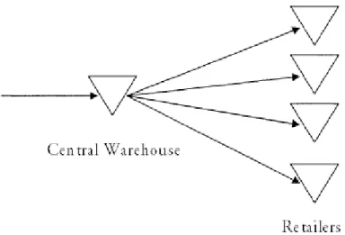
There exist many different multi-echelon inventory systems and an example is a two-level distribution system that can be seen in Figure 8 below, this is the system considered in this master thesis. The system consists of two levels where the central warehouse represents one level and a number of parallel retailers represent the second level. One thing that distinguishes a distribution system is that each layer has exactly one predecessor. The best allocation of stock level between the different layers in the multi-echelon distribution system depends on the system structure, demand variations, lead times and different cost functions. (Axsäter, 1991, pp. 108-109).
27
Figure 8 – A multi-echelon distribution system
3.4.1 Determine a reorder point in multi-echelon inventory systems
Some theoretical results on how the exact cost can be determined for a one-warehouse-multi-retailer system with a (R,Q)-policy exist. An example can be seen in (Axsäter, 2000). The drawback for this exact method is that it becomes computationally complex and it is almost impossible to use for larger systems with high demand and/or many retailers.
The analytical model used in this project to calculate the reorder points in a multi-echelon inventory system is based on an approximation and is therefore not an exact technique to determine the reorder points. The results will not be as good as for the exact model. However, the analytical model will work for larger systems with high demand and/or many retailers. The analytical model will be described in the following sections. The model, which is designed and developed at the division of Production Management at Lund University, is based on the research presented in three different research articles. All articles use an induced backorder cost at the central warehouse the differences are how this cost is determined and certain model assumptions. In the first article the backorder cost is determined through an iterative procedure in a multi-echelon inventory system with identical retailers and were the stochastic lead-times at the retailers are replaced with the correct averages obtained with Little’s formula (Andersson, Axsäter, & Marklund, 1998). The second article uses the same procedure but in a model with non-identical retailers, the average lead-time is then more complicated to compute and approximations are used (Andersson & Marklund, 2000). The third and last article examines how a simple closed form expression for estimating an induced
28
backorder cost of the central warehouse which makes the model conceptually and computationally simpler to use (Berling & Marklund, 2006). In section 3.5, there is a more thorough description of how this analytic model works.
3.5 Model for heuristic coordination of a decentralized
inventory system
Before the analytical model is described in detail, the inventory system and the assumptions made will be explained. All the assumptions made are from the three articles described in section 3.4.1. During the following description of the analytical model, the notations below will be used:
𝑁𝑁: number of retailers
𝑄𝑄: largest common divisor of all order quantities in the system 𝑞𝑞𝑖𝑖: order quantity at retailer 𝑖𝑖, expressed in units of 𝑄𝑄
𝑄𝑄𝑖𝑖: order quantity at retailer 𝑖𝑖, expressed in number of units (𝑄𝑄𝑖𝑖 = 𝑞𝑞𝑖𝑖𝑄𝑄)
𝑄𝑄0: warehouse order quantity, expressed in units of 𝑄𝑄 ℎ0: holding cost per unit and time unit at the warehouse ℎ𝑖𝑖: holding cost per unit and time unit at retailer 𝑖𝑖 𝑝𝑝𝑖𝑖: shortage cost per unit and time unit at retailer 𝑖𝑖
𝐼𝐼0: constant lead-time for an order to arrive at the warehouse
𝑙𝑙𝑖𝑖: constant transportation time between the warehouse and retailer i 𝐼𝐼𝑖𝑖: lead-time for an order to arrive at retailer 𝑖𝑖
𝐼𝐼�𝑖𝑖: expected lead-time for an order to arrive at retailer 𝑖𝑖
𝐷𝐷𝑖𝑖(𝑡𝑡): customer demand at retailer 𝑖𝑖 during time period 𝑡𝑡, stochastic variable
𝜇𝜇𝑖𝑖: expected demand per time unit at retailer 𝑖𝑖
𝜇𝜇0: expected demand per time unit at the warehouse = ∑𝑁𝑁𝑖𝑖=1𝜇𝜇𝑖𝑖 𝜎𝜎𝑖𝑖: standard deviation of the demand per time unit at retailer 𝑖𝑖
𝐷𝐷0(𝑡𝑡): retailer demand at the warehouse during the time period 𝑡𝑡, stochastic variable
𝑅𝑅𝑖𝑖: reorder point for retailer 𝑖𝑖
𝑅𝑅0: warehouse reorder point in units of 𝑄𝑄
𝐵𝐵0𝑖𝑖(𝑅𝑅0): expected number of backordered units at the warehouse designated for retailer 𝑖𝑖 when the reorder point is 𝑅𝑅0
𝐵𝐵0(𝑅𝑅0): expected number of backordered units at the warehouse given 𝑅𝑅0 𝐶𝐶𝑖𝑖: expected cost per time unit at retailer 𝑖𝑖
29
𝑇𝑇𝐶𝐶: expected total system cost per time unit
The model deals with an inventory system with one central warehouse and N retailers; similar to the inventory system described in Figure 8. Customer demand in the system takes place at the retailers who replenish their stocks from the central warehouse. Transportation times from the central warehouse to the retailers are considered to be constant, but delays may occur due to stockouts at the central warehouse. The perceived stochastic lead-times at the retailers are replaced by an estimate of their mean. The central warehouse replenishes its stock from an outside supplier where the lead time is constant, i.e. the supplier always has the required units in stock. Stockouts at all echelons is handled in accordance to a first-come-first-served policy and all facilities apply a (R,Q)-policy with continuous review. In addition partial deliveries are assumed.
The different costs that the model takes into account are the holding costs for all echelons and shortage costs at the retailers, which is proportional to the time until delivery. All orders quantities is considered to be predetermined and fixed, which results in that the only decision variables to be considered is the reorder points. This limitation can be considered as a weakness of the model, but in reality the order quantity often is limited by containers or pallet size. There are indications that the savings that can be obtained by varying the optimal order quantity is marginal given that the reorder points are properly set (Zheng, 1992). Furthermore, the initial inventory position, the reorder point and the batch size at the central warehouse are integer multiples of Q. The inventory position at the central warehouse is always non-negative, i.e. R0 ≥ -1 so that the maximum delay
is no more than L0. This is an original assumption, but the process in the model in
this master thesis cannot guarantee that R0 ≥ -1, so this assumption is not used.
This also means that an order placed at time t is independent of demand and retailer orders occurring after time t.
The objective with this model is to optimize the reorder points for the whole inventory system so that the total cost is minimized. This total cost for the system can be divided into two parts, the cost at the warehouse and at the different retailers:
𝑇𝑇𝐶𝐶 = 𝐶𝐶0+ � 𝐶𝐶𝑖𝑖 𝑁𝑁 𝑖𝑖=1