time-frequency representation
Cite as: Rev. Sci. Instrum. 90, 064901 (2019); https://doi.org/10.1063/1.5082776Submitted: 24 November 2018 . Accepted: 12 May 2019 . Published Online: 03 June 2019 Yongliang Cheng, Jie Shao, Yihe Zhao, Shu Liu, and Reza Malekian
ARTICLES YOU MAY BE INTERESTED IN
626-nm single-frequency semiconductor laser system operated near room temperature for
mW-level second-harmonic generation at 313 nm
Review of Scientific Instruments
90, 063201 (2019);
https://doi.org/10.1063/1.5096368
A ten-inch manipulator (TIM) based fast-electron spectrometer with multiple viewing
angles (OU-ESM)
Review of Scientific Instruments
90, 063501 (2019);
https://doi.org/10.1063/1.5088529
Viscosity measurements in pulsed magnetic fields by using a quartz-crystal microbalance
Review of Scientific Instruments
90, 065101 (2019);
https://doi.org/10.1063/1.5098451
An improved separation method
of multi-components signal for sensing
based on time-frequency representation
Cite as: Rev. Sci. Instrum. 90, 064901 (2019);doi: 10.1063/1.5082776
Submitted: 24 November 2018 • Accepted: 12 May 2019 • Published Online: 3 June 2019
Yongliang Cheng,1,2 Jie Shao,1,2 Yihe Zhao,1,2 Shu Liu,1,2 and Reza Malekian3,a)
AFFILIATIONS
1Key Laboratory of Radar Imaging and Microwave Photonics (Nanjing University of Aeronauts and Astronauts),
Ministry of Education, College of Electronic and Information Engineering, Nanjing University of Aeronautics and Astronautics, Nanjing 210016, China
2Key Laboratory of Underwater Acoustic Signal Processing, Ministry of Education, Southeast University, Nanjing 210096, China
3Department of Computer Science and Media Technology, Malmö University, Malmö 20506, Sweden and Internet of Things
and People Research Center, Malmö University, Malmö 20506, Sweden
a)E-mail:reza.malekian@ieee.org
ABSTRACT
In many situations, it is essential to analyze a nonstationary signal for sensing whose components not only overlapped in time-frequency domain (TFD) but also have different durations. In order to address this issue, an improved separation method based on the time-frequency distribution is proposed in this paper. This method computes the time-frequency representation (TFR) of the signal and extracts the instan-taneous frequency (IF) of components by a two-dimensional peak search in a limited area in which normalized energy is greater than the set threshold value. If there is more than one peak from a TFR, IFs of components can be determined and linked by a method of minimum slope difference. After the IFs are obtained, the improved time-frequency filtering algorithm is used to reconstruct the component of the signal. We continue this until the residual energy in the TFD is smaller than a fraction of the initial TFD energy. Different from previous methods, the improved method can separate the signal whose components overlapped in TFR and have different time durations. Simulation results have shown the effectiveness of the proposed method.
Published under license by AIP Publishing.https://doi.org/10.1063/1.5082776
I. INTRODUCTION
In many research fields, such as radar, sonar, and mechanical engineering, the signals received by sensors which have time-varying frequency contents are always multicomponent nonstationary sig-nals.1–5Therefore, it is necessary to separate components from the signal in order to effectively analyze them, some of which may overlap in the time-frequency domain (TFD).
Time-frequency representation (TFR) is a powerful processing tool for a multicomponent nonstationary signal. When dealing with the multicomponent signal, linear transform TFRs do not produce cross terms and have the advantage of low computation complexity. However, they are not robust to noise and have a low time-frequency resolution. Nonlinear transform TFRs overcome the drawback of
linear transform TFRs, but they suffer from serious cross terms. In order to obtain high time-frequency resolution and cross terms sup-pressed TFRs, a series of new time-frequency analysis methods are proposed in recent years.6–14
When a TFR is obtained, the instantaneous frequencies (IFs) of signal components can be extracted in the time-frequency domain. For a monocomponent signal, its IF is denoted by a thin and energy concentrative curve called “ridge.” By extracting the accurate posi-tion of the ridge, the IF of a signal can be got. However, how to extract IFs from the TFR of the multicomponent signal is still a problem, even if a noise free, cross terms are suppressed and high time-frequency resolution TFR is obtained.
In the past decades, many signal decomposition methods have been proposed to separate the multicomponent signal. Some
representative methods include the empirical mode decomposition and its improvement,15,16the synchrosqueezed wavelet transform,17 the empirical wavelet transform,18the variational mode decompo-sition,19 the nonlinear mode decomposition,20 data-driven time-frequency analysis,21sparse time-frequency decomposition,22 varia-tional nonlinear chirp mode decomposition,23adaptive chirp mode pursuit,24 and so on. However, most of the decomposition meth-ods require that the components of the signal satisfy strict separation conditions in their time-frequency plane, and thus, they cannot sep-arate close and overlapped signal components in the time-frequency plane completely.
Recently, some approaches are proposed in order to separate overlapped signal components. Barkat presents two signal separa-tion algorithms in Ref.25. One of them assumes that all compo-nents exist at all time instants in the time-frequency plane and any component intersection is a cross point. A method based on com-pressive sensing is put forward in Ref.26. It can effectively separate nonstationary and stationary signal components overlapping in the time-frequency plane. The intrinsic chirp component decomposi-tion (ICCD) in Ref.27can separate overlapped signal components by using a joint-optimization technique. A multicomponent signal separation method based on ridge path regrouping (RPRG) and ICCD is proposed in Ref.28. It can extract all IFs of components from TFR and regroups them using ridge path regrouping.
It can be found that separating multicomponent signals with overlapping components and different time durations is still a chal-lenging task for the methods above. To solve the issue, an improved method based on TFR is proposed in this paper. The method com-putes the TFR of the signal and extracts the IF of a component by finding the peaks of each time slice of TFR. Then, the minimum slope difference method is used to determine and link IF of time instants. Next, reconstruct the component by an improved time-frequency filtering method and remove it from the original signal. Finally, based on the improved energy criterion, the above steps are repeated for the residual signal until all components are extracted from the original signal.
This paper is organized as follows: In Sec.II, we briefly describe some IF separation methods of the multicomponent signal. Then, our improved method is proposed in Sec.III. In Sec.IV, simula-tion results and discussion of multicomponent signal separasimula-tion are provided to demonstrate the effectiveness of the proposed method. Finally, we draw a conclusion in Sec.V.
II. METHODS A. Signal model
A multicomponent nonstationary signal considered in this paper is S(t) = K ∑ k=1 Ak(t) exp[ j ⋅ φk(t)] + w(t), (1) where K is the number of signal components, Ak(t) and 𝜑k(t) denote the instantaneous amplitude (IA) and the instantaneous phase of kth signal components, respectively, and w(t) is a white Gaussian noise. B. Time frequency representation
To capture the time-varying signatures of the nonstationary signal, a TFR is needed. As the earliest TFR, short time Fourier
transform (STFT) is one of the most widely used TFR, which has the advantage of cross terms free and low computation complexity. STFT is defined as follows: TFR(t, f ) = STFT(t, f ) =∫ ∞ −∞gσ(τ)S(t + τ)e −j2πf τ dτ, (2)
where gσ(τ) is a Gaussian window with length of σ, S(t) is the sig-nal to be transformed, and TFR(t, f ) is the obtained TFR. When a TFR of the signal is obtained, IFs of the components can be extracted from it.
C. IFs extraction algorithm of multicomponent signal
IFs can be extracted by ridge detection from a TFR. The ridge detection finds a maximum energy point of the TFR in the frequency slice at each time instant and considers the corresponding frequency as the IF of current time instant. It can be denoted as
IF(t) = arg max F
∣TFR(t, F)∣, t = t0, . . . , tN−1, (3) where F is the set of frequency bins and N is the number of sampling points.
An efficient method sharing the idea of formula(3)proposed in Ref.25is introduced in Algorithm1, where TFR(t, f ) is the TFR of signal S(t), ∆f is the allowable frequency variation between two consecutive time instants, ε is the threshold of TFR energy, and IF(t) is the extracted IF.
This method can extract the IFs from the strongest to weak-est one by one. However, if there are overlapped areas of compo-nents in the time frequency plane, the method will fail to extract them.
In Ref.28, the RPRG first detects the ridges of a multicompo-nent signal from a TFR and then extracts the desired IFs by regroup-ing the ridge curves accordregroup-ing to their variation rates at the intersec-tions. After the IFs are obtained, component separation is achieved by using ICCD.
III. IMPROVED SEPARATION METHOD OF MULTICOMPONENTS SIGNAL
The RPRG + ICCD method can separate the overlapped com-ponents in the time-frequency domain completely. However, it can-not separate the components existing at different time periods well and mixes unexpected frequencies.
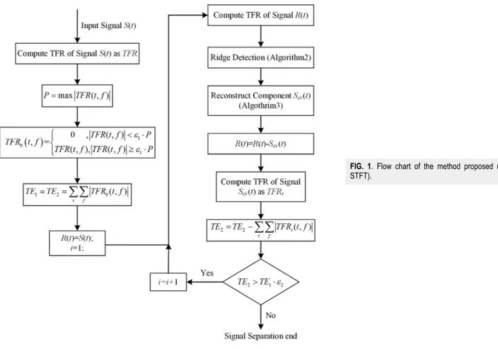
With the aid of a method that stops the extraction algorithm in Ref.24, a new adaptive energy criterion based on residual time fre-quency energy is proposed. The flow chart of the improved method is given inFig. 1.
The first step of the algorithm consists in noise thresholding to remove the undesired “low” energy peaks in the time-frequency domain and obtain the original total energy TE1, where ε1 is a properly selected threshold (in our simulations, we used ε1= 0.05). Then, the various components are extracted sequentially. Normally, the overall energy in the TFR becomes smaller and smaller after each extraction and after the last component has been retrieved the remaining energy in the TFR matrix should be a fraction of the original one. It is the energy criterion that stops the extraction algorithm.
ALGORITHM 1. Components separation procedure proposed in Ref.25. Input: TFR(t, f ), ∆f, ε
1: Compute total time-frequency energy TE1= N−1 ∑ i=0 M−1 ∑ j=0
∣TFR(ti, fj)∣, where M is the point number of Fourier transform. 2: Find (tmax, fmax) =arg max
t,f
∣TFR(t, f )∣, and set TFR(tmax, F), F ∈ [ fmax− ∆f, fmax+ ∆f ] 3: Initialize the center frequencies of searching to the left and right fL= fR= IF(tmax) = fmax 4: for r = max + 1, ⋯, N−1, and l = max − 1, ⋯, 0
5: IF(tr) =fR= arg max F∈[ fR−∆f ,fR+∆f ]
∣TFR(tr, F)∣, and then set TFR(tr, F), F ∈ [fR− ∆f, fR+ ∆f ] 6: IF(tl) =fL= arg max
F∈[ fL−∆f ,fL+∆f ]
∣TFR(tl, F)∣, and then set TFR(tl, F), F ∈ [fL− ∆f, fL+ ∆f ] 7: Compute the remaining time-frequency energy TE2=
N−1 ∑ i=0 M−1 ∑ j=0∣TFR(ti, fj)∣ 8: If TE2>TE1⋅ε
9: Jump to step 2 to start a new component extraction. 10: Else
11: stop component separation.
Output: IF(t), t = t0, ⋯, tN−1
A. Improved ridge detection algorithm
IF can be extracted by formula(3)for the monocomponent sig-nal, but it is not suitable for the multicomponent signal. It can be modified to search local maxima also known as the peaks of F rather
than the maximum of F. It is denoted as
Fi(t) = arg maxiam F
∣TFR(t, F)∣, t = t0, . . . , tN−1, (4) where i is the number of peaks at time instant t.
FIG. 1. Flow chart of the method proposed (TFR, e.g.,
FIG. 2. Illustration of the possible detected ridge points for two overlapped
components.
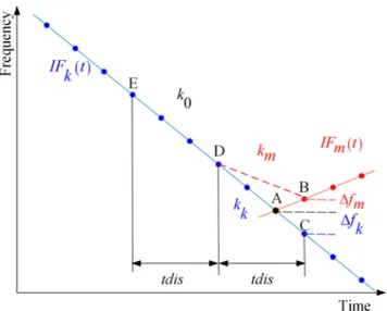
The possible detected ridge points for two overlapped compo-nents is illustrated inFig. 2, where IFk(t) and IFm(t) are the IFs of two crossed components and point A is the cross-point of compo-nents. Point B and point C are the peaks at the same time instant after point A, respectively. ∆fkand ∆fmare the frequency variation of points A, B and points A, C, respectively.
After cross-point A, many methods fail to extract IFs of the overlapped components correctly. For Algorithm1, when ∆fk<∆f, ∆fm<∆f and the amplitude of point B is greater than that of point C, the frequency of point B will be considered as the frequency of com-ponent k, so comcom-ponents k and m cannot be accurately identified. The peak frequencies of points B and C can be obtained by formula
(4). We can compute the minimum distance between them and the frequency of time instant of point A. However, if ∆fm<∆fk, the fre-quencies of component m may be mixed into those of component k. To avoid this drawback, we introduce the minimum slope difference method.
Usually, for the continuous frequency modulated signal, its fre-quency variation in a short time can be considered as linear. Based on this assumption, the adjacent points with nearly equal slope should be considered as belong to the same component.
As shown inFig. 2, our method computes slope differences of ED, DB and ED, DC, respectively. They are denoted as follows:
slopdk= ∣k0−kk∣, (5) slopdm= ∣k0−km∣, (6) k0=IF(tE) −IF(tD) tdis , (7) km=IF(tD ) −IF(tB) tdis , (8) kk=IF(tD ) −IF(tC) tdis , (9)
where tdis is the time interval between point E to point D and is set to 3%–5% of signal length N.
slopdk is obviously smaller than slopdm, so the frequency of point C should be considered as the frequency of component k rather than component m. Finally, the IF of component k can be extracted completely and correctly.
The ridge detection procedure is introduced in Algorithm2, where inds and inde are the indices of the start time and end time of a component, respectively. thres is the threshold of amplitude when finding the peaks in limited area, trb and tlb save the time instants whose number of peaks is zero, tb is the maximum allow-able breakpoint range, and if there is no peak at a set of con-secutive time instants whose length is greater than tb, the com-ponent is considered as an appearing end point or start point, respectively.
B. Component reconstruction based on improved time frequency filtering
A component can be reconstructed by combining the instan-taneous amplitude (IA) with the instaninstan-taneous phase. The instanta-neous phase can be achieved by the integral of IF. IF extracted from a TFR is not accurate because of the influence of the noise, and the frequency bins of IF are fixed. So, IF should be smoothed to obtain a more accurate instantaneous phase. A modified second difference matrix 𝛀 is used to smooth IF in Ref.23. IA extraction algorithm can be utilized by integrating dechirp with a low-pass filter.29The time frequency filtering algorithm is improved to filter the dechirp signal ranging from tindsto tinde.
The component reconstruction procedure is introduced in Algorithm3, where IF(t), inds, and inde are the IF, start time index, and end time index of the component obtained by Algorithm2, respectively, and β is the smooth coefficient.
IV. RESULTS AND DISCUSSION
In this section, some numerical results are provided for demon-strating the advantages of the proposed method.
A. Simulation and parameter settings
All the tests are carried out using MATLAB 2016a. The sam-ple frequency fs is 1000 Hz, the signal length N is 1000, and the frequency bins of FFT are 1024. The number of Monte Carlo sim-ulations is 100. The threshold of time frequency energy ε1= 0.05 and ε2= 0.1.
B. Quantitative results
To quantitatively compare the performances of algorithms, the mean absolute error (MAE) and mean squared error (MSE) are introduced.30They are defined as follows:
MAE = 1 N N−1 ∑ n=0 ∣IFe(tn) −IFo(tn)∣, (10) MSE = 1 N N−1 ∑ n=0 ∣IFe(tn) −IFo(tn)∣2, (11) where IFe(t) is the IF extracted and IFo(t) is the true IF.
ALGORITHM 2. Ridge detection. Input: TFR(t, f ), ∆f, tdis, thres
1: Find (tm, fm) = arg max t,f
∣TFR(t, f )∣, and let fL= fR= IF(ttm) = fm 2: Normalize TFR(t, f ), TFD(t, f ) =max∣TFR(t,f )∣∣TFR(t,f )∣
3: Initialize inds = 0, inde = N− 1, j = tm + 1, k = tm − 1, trb = tlb = [], tb = 0.3N 4: While j ≤ N− 1 do
5: Fi(tj)← Argument of maxima of TFD(ti, F), F ∈ [fR− ∆f, fR+ ∆f ] whose amplitude is greater than thres. 6: if i == 0 do
7: trb = [trb, j], tx = min{⌊( j − tm)/2⌋, tdis},IF(tj) = fR= IF(tj−tx) + [IF(tj−tx)− IF(tj−2tx)], j = j + 1 8: else if i == 1 do
9: IF(tj) = fR= F1(tj), j = j + 1
10: else
12: tx = min{⌊( j − tm)/2⌋, tdis}, IF(tj) =fR=arg max Fi(tj)
∣Fi(tj)−IF(ttx j−tx)−IF(tj−tdis)−IF(ttx j−2tx)∣, j = j + 1 13:inde ← continues breakpoints analysis of trb
14: While k ≥ 0 do
15: Fi(tk) ← Argument of maxima of TFD(tj, F), F ∈ [fL− ∆f, fL+ ∆f ] whose amplitude is greater than thres. 16: if i == 0 do
17: tlb = [tlb, k], tx = min{⌊(inde − k)/2⌋, tdis}, IF(tk) = fL= IF(tk−tx) + [IF(tk−tx)− IF(tk−2tx)], k = k− 1 18: else if i == 1 do
19: IF(tk) = fL= F1(tk), k = k− 1
20: else
21: tx = min{⌊(inde − k)/2⌋, tdis}, IF(tk) =fL=arg max Fi(tk)
∣Fi(tk)−IF(ttx k+tx)−IF(tk+tx)−IF(ttx k+2tx)∣, k = k− 1 22:inds ← continues breakpoints analysis of tlb
Output: IF(t), t = t0, ⋯, tN−1, inds, inde 1. Example 1
A three-component nonstationary signal is described as fol-lows: S1(t) = Sc1(t) + Sc2(t) + Sc3(t) + w(t), (12) Sc1(t) = A1(t) exp[j2π(200t2)], 0 ≤ t ≤ 1s, (13) Sc2(t) = A2(t) exp[j2π(−200t + 150t3)], 0 ≤ t ≤ 1s, (14) Sc3(t) = ⎧ ⎪ ⎪ ⎨ ⎪ ⎪ ⎩ 0, 0 ≤ t < 0.1s A3(t) exp[j2π(400t − 200t2)], 0.1s ≤ t ≤ 1s, (15) where w(t) is noise, A1(t) = 1, A2(t) = e−0.5t, and A3(t) = 0.8 ⋅ e0.5t. ALGORITHM 3. Component reconstruction.
Input: IF(t), inds, inds, β, S(t)
1: Effective IF IFnew←(IF(t)−M/2)fM s, tinds≤t ≤ tiinde 2: Compute effective IF length L = inde− inds + 1
3: Initialize modified second difference matrix Ω = ⎡ ⎢ ⎢ ⎢ ⎢ ⎢ ⎢ ⎢ ⎢ ⎢ ⎣ −1 1 0 ⋯ 0 1 −2 1 ⋯ 0 ⋮ ⋱ ⋱ ⋱ ⋮ 0 ⋯ 1 −2 1 0 ⋯ 0 1 −1 ⎤ ⎥ ⎥ ⎥ ⎥ ⎥ ⎥ ⎥ ⎥ ⎥ ⎦L×L 3: Smooth effective IF Fsmooth= (2βΩTΩ+ I)
−1
IFnew, where T is the matrix transpose. 4: phase(tinds) = 2πFsmooth(1)
5: for ii = 2 to L
6: phase(tinds+ii−1) =phase(tinds+ii−2)+ 2πFsmooth(ii)+F2fsmooth(ii−1) s 7: end for
8: Dechirp Sd(t) = S(t) ⋅ e−j⋅phase(t ), tinds≤t ≤ tinde
9: IA(t), tinds≤t ≤ tinde←Estimated by low-pass filter of Sd(t) 10: Component reconstruction ˆSc(t) = IA(t) ⋅ e−j⋅phase(t), tinds≤t ≤ tinde
FIG. 3. Signal S1(t). (a) Waveform in the time domain. (b) TFR based on STFT.
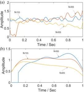
The waveform in the time domain and TFR based on STFT of signal S1(t) when SNR = 5 dB are exhibited inFig. 3. The IFs of sig-nal S1(t) separated by the proposed method and RPRG + ICCD are displayed inFig. 4. As shown inFig. 4, both methods can extract all components of signal S1(t). The difference is that the proposed method can identify the start-point of component Sc3(t) and set the frequencies as zero between 0 s and 0.1 s, while RPRG + ICCD mixes unexpected frequencies into Sc3(t).
The IAs extracted by RPRG + ICCD and the proposed method are displayed inFig. 5. As shown inFig. 5, the amplitude of IAs extracted by RPRG + ICCD fluctuates comparatively around the true IAs. The amplitude of IAs extracted by the proposed method fits the true IAs well. However, the error of IAs is large near the end point
FIG. 4. Extracted IFs of signal S1(t). (a) RPRG + ICCD. (b) The proposed method.
FIG. 5. Extracted IAs of signal S1(t). (a) RPRG + ICCD. (b) The proposed method.
because there are the edge effects of the low-pass filter and the time frequency energy of TFR is not concentrated at the end point.
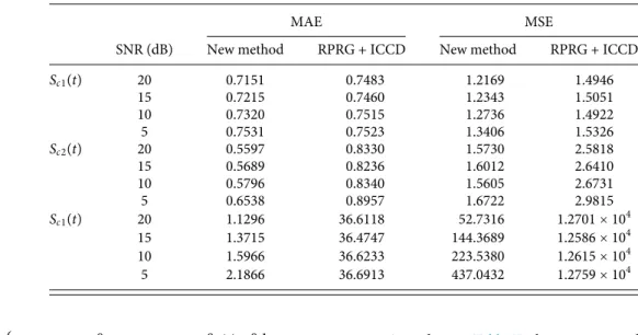
In order to compare the proposed method with the RPRG + ICCD quantitatively, the MAE and MSE of components of signal S1(t) under the different SNR are listed inTable I. For component Sc1(t), the MAE and MSE of a new method are slightly less than those of RPRG + ICCD under the conditions of SNR ranging from 10 dB to 20 dB, and the MAE and MSE of the new method are almost equal to those of RPRG + ICCD when SNR = 5 dB.
The MAE and MSE for component Sc2(t) of the proposed approach when SNR = 5 dB are reduced 27% and 44% than those of RPRG + ICCD. 20% listed inTable Imeans there is a 20% fail-ure rate of RPRG + ICCD when extracting this component (they are excluded when calculating MAE and MSE).
When SNR = 10 dB, the results of component Sc3(t) show that the MAE and MSE of the proposed method are about 35 and 12 400 fewer than those of RPRG + ICCD, respectively. It means that the proposed method can extract component Sc3(t) effectively, while RPRG + ICCD could not. Because the time frequency energy is not concentrated at the end of component Sc3(t), the MAE and MSE of component Sc3(t) obtained by the new method are obviously greater than those of components Sc1(t) and Sc2(t).
2. Example 2
A four-component nonstationary signal is given as follows: S2(t) = Sc1(t) + Sc2(t) + Sc3(t) + Sc4(t) + w(t), (16)
Sc1(t) = A1(t) exp[j2π(200t2)], 0 ≤ t ≤ 1s, (17) Sc2(t) = A2(t) exp{ j2π[140t + 150 sin(2πt)]}, 0 ≤ t ≤ 1s, (18)
Sc3(t) = ⎧ ⎪ ⎪ ⎨ ⎪ ⎪ ⎩ A3(t) exp{ j2π[−140t − 150 sin(2πt)]}, 0 ≤ t ≤ 0.9s 0, 0.9 s < t ≤ 1s, (19)
TABLE I. The MAE and MSE of IFs under different SNR.
MAE MSE
SNR (dB) New method RPRG + ICCD New method RPRG + ICCD
Sc1(t) 20 0.7151 0.7483 1.2169 1.4946 15 0.7215 0.7460 1.2343 1.5051 10 0.7320 0.7515 1.2736 1.4922 5 0.7531 0.7523 1.3406 1.5326 Sc2(t) 20 0.5597 0.8330 1.5730 2.5818 15 0.5689 0.8236 1.6012 2.6410 10 0.5796 0.8340 1.5605 2.6731 5 0.6538 0.8957 1.6722 2.9815 Sc1(t) 20 1.1296 36.6118 52.7316 1.2701 × 10⁴ 15 1.3715 36.4747 144.3689 1.2586 × 10⁴ 10 1.5966 36.6233 223.5380 1.2615 × 10⁴ 5 2.1866 36.6913 437.0432 1.2759 × 10⁴ Sc4(t) = ⎧ ⎪ ⎪ ⎨ ⎪ ⎪ ⎩ 0, 0 ≤ t < 0.1s A4(t) exp[j2π(400t − 200t2)], 0.1s ≤ t ≤ 1s, (20) where A1(t) = 1, A2(t) = e−0.4t, A3(t) = 1 + 0.3 cos(2πt + π/2), and A4(t) = 0.8⋅e0.4t.
The waveform in the time domain and TFR based on STFT of signal S2(t) when SNR = 10 dB are depicted inFig. 6. The IFs of signal S2(t) separated by the proposed method and RPRG + ICCD are illustrated inFig. 7. It can be seen that both methods separate all components of signal S2(t). The proposed method can correctly extract the component Sc4(t) which starts at time 0.1 s and the com-ponent Sc3(t) which ends at time 0.9 s, while RPRG + ICCD could not.
The MAE and MSE of components of signal S2(t) under the condition of different SNR are listed inTable II.
FIG. 6. Signal S2(t). (a) Waveform in the time domain. (b) TFR based on STFT.
According toTable II, the superiority of MAE and MSE for components Sc1(t) and Sc2(t) in the proposed approach is not obvi-ous. However, RPRG + ICCD cannot extract components Sc2(t) and Sc3(t) when SNR = 5 dB. When SNR = 10 dB, the MAEs of com-ponents Sc3(t) and Sc4(t) obtained by an improved approach are 3.0763 and 1.9614, and those of Sc3(t) and Sc4(t) by RPRG + ICCD are 19.3987 and 36.2974, respectively. It is demonstrated that the proposed method almost completely extracts components Sc3(t) and Sc4(t), while RPRG + ICCD fails to do it.
3. Example 3
This example is still a four-component signal, which is described as follows:
S3(t) = Sc1(t) + Sc2(t) + Sc3(t) + Sc4(t) + w(t), (21)
TABLE II. The MAE and MSE of IFs under different SNR.
MAE MSE
SNR (dB) New method RPRG + ICCD New method RPRG + ICCD
Sc1(t) 20 0.7637 0.7655 1.2376 1.4519 15 0.7723 0.7580 1.2720 1.4467 10 0.7631 0.7606 1.2479 1.4425 5 0.7607 0.7670 1.2383 1.4944 Sc2(t) 20 0.9942 0.9819 1.6337 2.4743 15 1.0232 0.9740 1.8219 1.8292 10 1.0217 1.0135 1.8404 1.7385 5 1.0707 NA 2.1818 NA Sc3(t) 20 2.9389 19.6054 386.0232 3.4958 × 10³ 15 2.9909 19.3327 393.6796 3.3914 × 10³ 10 3.0763 19.3987 406.2418 3.4060 × 10³ 5 3.1884 NA 421.1892 NA Sc4(t) 20 1.6299 36.4080 210.2445 1.2570 × 10⁴ 15 1.8229 36.6571 292.6739 1.2763 × 10⁴ 10 1.9614 36.2974 353.1569 1.2466 × 10⁴ 5 2.2637 36.3920 459.6359 1.2546 × 10⁴ Sc1(t) = A1(t) exp[j2π(200t2)], 0 ≤ t ≤ 1 s, (22) Sc2(t) = ⎧ ⎪ ⎪ ⎨ ⎪ ⎪ ⎩
A2(t) exp{ j2π[140t + 150 sin(2πt)]}, 0 ≤ t ≤ 1 s
0, 0.15 s < t ≤ 1 s, (23) Sc3(t) = ⎧ ⎪ ⎪ ⎨ ⎪ ⎪ ⎩ A3(t) exp{ j2π[−140t − 150 sin(2πt)]}, 0 ≤ t ≤ 0.9 s 0, 0.9 s < t ≤ 1 s, (24)
FIG. 8. Signal S3(t). (a) Waveform in the time domain. (b) TFR based on STFT.
Sc4(t) = ⎧ ⎪ ⎪ ⎨ ⎪ ⎪ ⎩ 0, 0 ≤ t < 0.1 s A4(t) exp[j2π(400t − 200t2)], 0.1 s ≤ t ≤ 1 s, (25) where A1(t) = A3(t) = 1, A2(t) = e−0.4t, and A4(t) = 0.8 ⋅ e0.4t.
The waveform in the time domain and TFR based on STFT of signal S3(t) when SNR = 20 dB are shown in Fig. 8. The IFs of signal S3(t) separated by the proposed approach and RPRG + ICCD are presented in Fig. 9. As shown in Fig. 9, it can be clearly seen that both methods can achieve the extrac-tion of all components of signal S3(t). The proposed method extracts the components with different durations completely, while
TABLE III. The MAE and MSE of IFs under different SNR.
MAE MSE
SNR (dB) New method RPRG + ICCD New method RPRG + ICCD
Sc1(t) 20 0.7683 0.7632 1.3328 1.5097 15 0.7710 0.7711 1.3255 1.5467 10 0.7744 0.7743 1.3338 1.5521 5 0.7823 0.7757 1.3395 1.6086 Sc2(t) 20 3.0633 23.7196 326.7530 3.4913 × 10³ 15 3.0402 24.3193 322.5048 3.6558 × 10³ 10 3.1028 23.6586 328.3039 3.4614 × 10³ 5 3.3733 24.6332(20%) 358.2955 3.6633 × 10³(20%) Sc3(t) 20 2.6421 19.2998 341.8645 3.3916 × 10³ 15 2.7015 19.3194 352.6694 3.3987 × 10³ 10 2.8760 19.2338 381.7343 3.3616 × 10³ 5 3.2185 19.3058 442.3798 3.3639 × 10³ Sc4(t) 20 1.7250 36.9284 249.6887 1.2940 × 10⁴ 15 1.6732 36.5844 234.6703 1.2686 × 10⁴ 10 1.8922 36.3784 329.0008 1.2537 × 10⁴ 5 2.1345 36.6176 422.0073 1.2656 × 10⁴
RPRG + ICCD mixes undesirable frequencies into components Sc2(t), Sc3(t), and Sc4(t).
The MAE and MSE of components of signal S3(t) in the pro-posed method and the RPRG + ICCD are provided in Table III. With the decrease in SNR, the MAE and MSE of component Sc1(t) gradually increase. Due to the existence of start time or end time in components Sc2(t), Sc3(t), and Sc4(t), the MAE and MSE of the pro-posed method are clearly smaller than those of RPRG + ICCD. It is demonstrated inTable IIIthat the proposed method is superior to RPRG + ICCD under the same condition of noise.
V. CONCLUSION
In this paper, an improved separation method of the multicom-ponent signal for sensing based on time-frequency representation is proposed in order to separate the signal whose components over-lapped in the time-frequency domain and have different time dura-tions. This method first computes the TFR of the signal and extracts the instantaneous frequency of a component by a ridge detection procedure based on the minimum slope difference algorithm. Then, reconstruct the component by an improved time-frequency filtering algorithm. By this, a complete component is extracted and then the extracted component is subtracted from the original signal. Finally, based on the improved energy criterion, the above steps are repeated for the residual signal to separate all components one by one.
To show the effectiveness of the proposed method, we ana-lyzed some simulated multicomponent signals. When there are com-ponents of the signal throughout the period of time, the perfor-mance of the proposed method is similar to that of RPRG + ICCD for linear frequency modulation (LFM) signals. However, for the high order frequency modulation signal, such as the quadratic fre-quency modulation (QFM) and sinusoidal frefre-quency modulation (SFM) signal, the improved method performs obviously better than
RPRG + ICCD. When the components of a signal do not exist at all time instants, the MAE and MSE of our approach can be reduced by up to 89% and 90%, respectively, in comparison with the RPRG + ICCD. IFs extraction is improved significantly by our method.
Simulation and experimental results have demonstrated the superiority of the proposed algorithm to separate the signal whose components have different durations and overlapped in the time-frequency domain. After the signal components are effectively separated, the parameters of the components can be estimated accurately.
ACKNOWLEDGMENTS
This work was supported in part by the Open Project Program of the Key Laboratory of Underwater Acoustic Signal Processing (Southeast University), China’s Ministry of Education (Grant No. UASP1604), and the Fundamental Research Funds for the Central Universities (Grant No. 2242016K3001), a project funded by the Pri-ority Academic Program Development of Jiangsu Higher Education Institutions.
The authors declare that they have no competing interests. NOMENCLATURE
TFR time frequency representation IFs instantaneous frequencies
ICCD intrinsic chirp component decomposition RPRG ridge path regrouping
STFT short time Fourier transform
IA instantaneous amplitude
MAE mean absolute error
MSE mean square error
QFM quadratic frequency modulation SFM sinusoidal frequency modulation REFERENCES
1Z. Feng, M. Liang, and F. Chu, “Recent advances in time–frequency analysis methods for machinery fault diagnosis: A review with application examples,”
Mech. Syst. Signal Process.38(1), 165–205 (2013).
2S. K. Hadjidimitriou and L. J. Hadjileontiadis, “Toward an EEG-based recogni-tion of music liking using time-frequency analysis,”IEEE Trans. Biomed. Eng.
59(12), 3498–3510 (2012).
3Z. K. Peng, G. Meng, F. L. Chu et al., “Polynomial chirplet transform with appli-cation to instantaneous frequency estimation,”IEEE Trans. Instrum. Meas.60(9), 3222–3229 (2011).
4B. Boashash and S. Ouelha, “An improved design of high-resolution quadratic time–frequency distributions for the analysis of nonstationary multicomponent signals using directional compact Kernels,”IEEE Trans. Signal Process.65(10), 2701–2713 (2017).
5
X. J. Jin, J. Shao, X. Zhang, W. W. An, and R. Malekian, “Modeling of nonlin-ear system based on deep lnonlin-earning framework,”Nonlinear Dyn.84(3), 1327–1340 (2016).
6
N. A. Khan and B. Boashash, “Instantaneous frequency estimation of multicom-ponent nonstationary signals using multiview time-frequency distributions based on the adaptive fractional spectrogram,”IEEE Signal Process. Lett.20(2), 157–160 (2013).
7B. Boashash, N. A. Khan, and T. Ben-Jabeur, “Time–frequency features for pat-tern recognition using high-resolution TFDs: A tutorial review,”Digital Signal Process.40(C), 1–30 (2015).
8N. A. Khan and B. Boashash, “Multi-component instantaneous frequency esti-mation using locally adaptive directional time frequency distributions,”Int. J. Adapt. Control Signal Process.30(3), 429–442 (2016).
9Z. Xin, S. Jie, A. Wenwei et al., “An improved time-frequency representation based on nonlinear mode decomposition and adaptive optimal Kernel,”Elektron. Elektrotech.22(4), 52–57 (2016).
10S. R. Raj and P. R. Bilas, “Improved eigenvalue decomposition-based approach for reducing cross-terms in Wigner–Ville distribution,” Circuits, Syst., Signal Process.37(8), 3330–3350 (2018).
11P. Singh, “Novel Fourier quadrature transforms and analytic signal represen-tations for nonlinear and non-stationary time series analysis,”R. Soc. Open Sci.
5(11), 1–22 (2018).
12M. Mohammadi, A. A. Pouyan, N. A. Khan et al., “Locally optimized adaptive directional time–frequency distributions,”Circuits, Syst. Signal Process.37(8), 3154–3174 (2018).
13R. R. Sharma and R. B. Pachori, “Eigenvalue decomposition of Hankel matrix-based time-frequency representation for complex signals,”Circuits, Syst., Signal Process.37(8), 3313–3329 (2018).
14
R. R. Sharma and R. B. Pachori, “Time-frequency representation using IEVDHM-HT with application to classification of epileptic EEG signals,”IET Sci., Meas. Technol.12(1), 72–82 (2017).
15
N. E. Huang, Z. Shen, S. R. Long et al., “The empirical mode decomposition and the Hilbert spectrum for nonlinear and non-stationary time series analysis,”Proc. R. Soc. London, Ser. A454(1971), 903–995 (1998).
16
K. T. Sweeney, S. F. Mcloone, and T. E. Ward, “The use of ensemble empir-ical mode decomposition with canonempir-ical correlation analysis as a novel artifact removal technique,”IEEE Trans. Biomed. Eng.60(1), 97–105 (2013).
17
I. Daubechies, J. Lu, and H. T. Wu, “Synchrosqueezed wavelet transforms: An empirical mode decomposition-like tool,”Appl. Comput. Harmonic Anal.30(2), 243–261 (2011).
18
J. Gilles, “Empirical wavelet transform,”IEEE Trans. Signal Process.61(16), 3999–4010 (2013).
19
K. Dragomiretskiy and D. Zosso, “Variational mode decomposition,”IEEE Trans. Signal Process.62(3), 531–544 (2014).
20
D. Iatsenko, P. V. Mcclintock, and A. Stefanovska, “Nonlinear mode decompo-sition: A noise-robust, adaptive decomposition method,”Phys. Rev.92(3), 1–25 (2015).
21
T. Y. Hou and Z. Q. Shi, “Data-driven time-frequency analysis,”Appl. Comput. Harmonic Anal.35(2), 284–308 (2013).
22T. Y. Hou and Z. Q. Shi, “Sparse time-frequency decomposition by dictionary adaptation,”Philos. Trans. R. Soc., A374(2065), 20150192 (2016).
23
S. Chen, X. Dong, Z. Peng et al., “Nonlinear chirp mode decomposi-tion: A variational method,” IEEE Trans. Signal Process.65(22), 6024–6037 (2017).
24
C. Shiqian, Y. Yang, P. Zhike et al., “Adaptive chirp mode pursuit: Algorithm and applications,”Mech. Syst. Signal Process.116, 566–584 (2019).
25B. Barkat and K. Abed, “Algorithms for blind components separation and extraction from the time-frequency distribution of their mixture,”EURASIP J. Adv. Signal Process.2004(13), 1–9.
26L. Stankovic, I. Orovic, S. Stankovic et al., “Compressive sensing based separa-tion of nonstasepara-tionary and stasepara-tionary signals overlapping in time-frequency,”IEEE Trans. Signal Process.61(18), 4562–4572 (2013).
27S. Chen, Z. Peng, Y. Yang et al., “Intrinsic chirp component decomposi-tion by using Fourier series representadecomposi-tion,”Signal Process.137(C), 319–327 (2017).
28S. Chen, X. Dong, G. Xing et al., “Separation of overlapped non-stationary sig-nals by ridge path regrouping and intrinsic chirp component decomposition,”
IEEE Sens. J.17(18), 5994–6005 (2017).
29Y. Yang, X. Dong, Z. Peng et al., “Component extraction for non-stationary multi-component signal using parameterized de-chirping and band-pass filter,”
IEEE Signal Process. Lett.22(9), 1373–1377 (2015).
30V. Sucic, J. Lerga, and B. Boashash, “Multicomponent noisy signal adaptive instantaneous frequency estimation using components time support informa-tion,”IET Signal Process.8(3), 277–284 (2014).