Master
's thesis • 30 credits
Agricultural programme – Economics and Management
Degree project/SLU, Department of Economics, 1266 • ISSN 1401-4084 Uppsala, Sweden 2019
Estimating the impact of agricultural support
on farm price
- an analysis of Swedish farm prices
Swedish University of Agricultural Sciences
Faculty of Natural Resources and Agricultural Sciences Department of Economics
Estimating the impact of agricultural support on farm price – an
analysis of Swedish farm prices
Maria Falkdalen
Supervisor: Helena Hansson, Swedish University of Agricultural Sciences, Department of Economics
Examiner: Jens Rommel, Swedish University of Agricultural Sciences, Department of Economics
Credits: 30 hec
Level: A2E
Course title: Master thesis in Economics
Course code: EX0907
Programme/Education: Agricultural programme –
Economics and Management 270,0 hec
Faculty: Faculty of Natural Resources and Agricultural Sciences
Place of publication: Uppsala
Year of publication: 2019
Name of Series: Degree project/SLU, Department of Economics
Part number: 1266
ISSN 1401-4084
Online publication: http://stud.epsilon.slu.se
iii
Acknowledgements
First of all, I would like to thank the Ministry of Enterprise and Innovation for the subject of this project and for providing valuable contacts for this thesis. I would also like to express gratitude to the people at the Swedish Board of Agriculture for the ability to get access to and analyse data of agricultural support. I would like to thank my supervisor Helena Hansson for guidance along the way. Finally, I would like to thank my family for the support during this project.
v
Abstract
Agricultural land prices in Sweden have been increasing steadily since Sweden joined the EU. At the same time, the common agricultural policy of the EU has changed from coupled
support given to specific sectors, to decoupled direct support for basic land maintenance. The need to understand the effects of agricultural policy decisions, how prices are determined and what factors are affecting agricultural land values, are therefore highly relevant and
interlinked topics.
The aim of this thesis was to analyse how the direct support in the EU’s common agricultural policy affects farm prices in Sweden by presenting a hedonic pricing model which can be used to estimate the effect of the direct support on farm prices. A broad literature review was performed regarding the capitalisation of agricultural support on land and farms and to gain an increased understanding about what factors are most likely to influence the farm price. Factors like the quality of the land, agricultural structure, urbanisation, agricultural policies and residential characteristics were found to be important determinants of the price of agricultural land and farms and were therefore included as independent variables in the analysis.
Data were analysed in STATA by multiple regression analysis where both pooled OLS, random effects and fixed effects regressions were used to determine the correlation between the independent variables and the dependent variable, the average farm price per municipality. The results from this study indicate that the decoupled direct payment has a significant
positive impact on the farm price. It also suggests that farm prices per municipality are on average 40 – 72 % higher after the introduction of the Single Farm Payment, compared to before the introduction. The prices are however not adjusted for inflation, therefore the results need to be interpreted with caution. The results from the study gives incentives for future research to further investigate the effect of different policy decisions.
vi
Sammanfattning
Sedan Sveriges inträde i EU har priset på jordbruksmark stigit kontinuerligt i Sverige. EU:s gemensamma jordbrukspolitik har samtidigt ändrats från kopplade stöd riktade till specifika sektorer, till frikopplade arealbaserade inkomststöd. Behovet av att förstå konsekvenserna av jordbrukspolitiska beslut och vilka faktorer som påverkar värdet på jordbruksmark är därför mycket viktiga och relaterade ämnen.
Syftet med den här uppsatsen var att analysera hur direktstöden i EU:s gemensamma
jordbrukspolitik påverkar gårdspriser i Sverige genom att presentera en hedonisk prismodell vilken kan användas för att uppskatta effekten av direktstöden på gårdspriser. En bred litteraturgenomgång genomfördes angående kapitaliseringen av jordbruksstöd i mark och gårdar och för att få en fördjupad förståelse för vilka faktorer som påverkar priset på gårdar. Viktiga faktorer som påverkar priset på jordbruksmark och gårdar är till exempel markens bördighet, strukturen i jordbruket, urbanisering, jordbrukspolitik och bostadsegenskaper, dessa faktorer inkluderades därför som förklarande variabler i analysen.
Data analyserades i STATA med hjälp av multipel regressionsanalys där både pooled OLS, random effects och fixed effects användes för att bestämma sambandet mellan de oberoende variablerna och den beroende variabeln, det genomsnittliga gårdspriset per kommun.
Resultaten från den här studien indikerar att det frikopplade direktstödet har en signifikant positiv påverkan på gårdspriset och att det genomsnittliga gårdspriset per kommun är mellan 40 – 72 % högre efter införandet av gårdsstödet, jämfört med innan. Priserna är dock inte justerade för inflation, vilket gör att resultaten måste tolkas med försiktighet. Resultaten från studien ger incitament till fortsatta studier för att undersöka effekten av olika politiska beslut.
vii
Abbreviations
CAP – Common Agricultural Policy EU – European Union
SEK – Swedish krona SFP – Single Farm Payment SPS – Single Payment Scheme OLS – Ordinary Least Squares
ix
Table of Contents
1 INTRODUCTION ... 1
1.1 Problem background ... 1
1.2 Problem statement ... 3
1.3 Aim and reseach question ... 4
1.4 Contribution and delimitations ... 4
1.5 Structure of the report... 5
2 EMPIRICAL BACKGROUND ... 6
2.1 Single Payment Scheme ... 6
3 THEORETICAL PERSPECTIVE AND LITERATURE REVIEW ... 7
3.1 Literature review ... 7
3.1.1 Agricultural support payments ... 7
3.1.2 Farm price determinants ... 8
3.2 The hedonic price model ... 10
4 METHOD AND DATA... 12
4.1 Data ... 12
4.1.1 Variables ... 13
4.2 Modeling a hedonic price funtion ... 16
4.3 Regression analysis ... 17
4.3.1 Panel data ... 17
5 RESULTS ... 19
5.1 Pooled OLS ... 19
5.2 Random effects and fixed effects regression ... 21
6 DISCUSSION ... 23
7 CONCLUSIONS ... 26
x
List of figures
Figure 1. The evolution of CAP. ... 2
Figure 2. Price trend for arable land and pasture. ... 3
List of tables
Table 1. Reasons to excluded observations ... 13Table 2. Variables and definitions ... 14
Table 3. Summary statistics ... 15
Table 4. Results from the regression using Pooled OLS ... 19
1
1 Introduction
This chapter introduces the research problem and gives a brief explanation of the
development of the common agricultural policy (CAP) in the EU. The purpose and research question are also presented and in the end of the chapter the contribution and delimitations will be given together with a disposition of the thesis.
1.1 Problem background
Sweden became a member of the European Union in 1995. From being a country with its own policy for agriculture and food, it became a part of a common market and a shared policy with the other members of the EU. The common agricultural policy (CAP) was introduced in 1962 and is a partnership between agriculture and the society and between Europe and its farmers (European Commission, 2019a). It aims to:
Support farmers and improve agricultural productivity, so that consumers have a stable supply of affordable food;
Ensure that European Union (EU) farmers can make a reasonable living;
Help tackling climate change and the sustainable management of natural resources; Maintain rural areas and landscapes across the EU;
Keep the rural economy alive promoting jobs in farming, agri-foods industries and associated sectors.
Since its introduction, the policy has gone through several reforms. After World War 2, the focus was on producing enough food in the EU and the CAP thus originally consisted of market and price support that stimulated production (Jordbruksverket, 2018a). This eventually led to a surplus of agricultural products in the 1980’s and measures were introduced to bring production levels closer to what the market needed (European Commission, 2019a). The 1992 MacSharry Reform and the AGENDA 2000 Reform transformed price policy into area
payments and animal payments (Kilian et al. 2012). In 2003 there was a major reform of the CAP, which introduced the Single Payment Scheme (SPS), where area and animal-specific payments were converted into the Single Farm Payment (SFP). This new system of decoupled direct support to farmers replaced most of the earlier coupled agricultural support to specific sectors. It was introduced in Sweden in 2005 (Jordbruksverket, 2011). By removing the link between subsidies and any specific production, the farmers are free to produce according to the market demand and at the same time get an income support. Figure 1 shows the
development of the CAP in the EU. As can be seen in the figure, the amount of coupled direct support has decreased since 2005 and has almost totally been replaced by the decoupled direct support.
2
Figure 1. The evolution of CAP (European Commission, 2019b).
Since the aim of the CAP is to promote agricultural development, there is a need to
understand how the current policy affects the agricultural development in Sweden. Several studies have been made in order to estimate the impact of different agricultural governmental support on agricultural land values (Goodwin and Ortalo-Magné, 1992; Barnard et al. (1997);
Kilian et al. (2012); Karlsson and Nilsson, (2014)).There is a consensus in the empirical
literature that agricultural support payments are important in explaining agricultural land prices (Latruffe and Le Mouël, 2009). Many of these studies are based on American
conditions, although the number of empirical studies based on European land markets have grown in number since the introduction of the decoupling reform in 2003. The applicability of the conclusions arising from American studies to countries in the EU is questionable due to important differences in the nature of government support between the US and the EU (Patton et al., 2008). There may also be differences in for example laws regarding land ownership or the interest for living on the countryside, between different countries. It is thus important to estimate the impact of CAP direct payments on land values in a Swedish context.
The 2003 common agricultural policy reform marks a significant change in European
agricultural policy and has changed the policy environment where farmers operate (Karlsson and Nilsson, 2014). The introduction of an annual Single Farm Payment (SFP) for basic land maintenance has contributed to raise several questions when it comes to understanding the effects of decoupled policies on European land markets and individual farmers. It is highly relevant for policy makers to understand the implications of policy decisions on the market, both for the evaluation of the current policy scheme, as well as in the process of reforming the CAP. The common agricultural policy is getting closer to a new program period, which will shape the new policy and which will apply in 2021 for seven years (Regeringskansliet, 2018). Sweden also has a national food strategy which aims to promote a sustainable and competitive
3 food chain in Sweden (Näringsdepartementet, 2017). Understanding how direct support and the SPS in the common agricultural policy affects agricultural land prices in Sweden are therefore a highly relevant and interesting subject.
1.2 Problem statement
Since Sweden joined the EU, the average prices for arable land and pasture have been increasing steadily (Jordbruksverket, 2018b). In 1995, the average price for arable land per hectare was 12 300 SEK, compared to 2016, when the price had increased to 75 000 SEK. The price for arable land had thus increased more than six times during those years. In 1995, the average price for permanent grassland per hectare was 4 300 SEK, compared to 2016, when the same amount of permanent grassland cost 28 000 SEK. The price trend can be seen in Figure 1, where the development for both arable land and pasture is shown. The price trend is made with an index for 1995 = 100. The blue colour represents arable land, while the orange colour represents pasture.
Figure 2. Price trend for arable land and pasture (Jordbruksverket, 2016).
The explanations for the increasing agricultural land prices in Sweden are likely to be related to both agricultural and urbanising factors (Nilsson and Johansson, 2013). Land can be seen as an important financial asset and insurance for farmers that allows for wealth accumulation and wealth transfer across generations. Higher land prices increase the wealth for those who own their land and can therefore be seen as beneficial for the individual land owner. A growth in land prices may however imply a higher barrier to entry into agricultural land markets for new farmers, as well as a higher cost for expanding farms (Hüttel et al., 2013). This leads to decreased sectoral efficiency. Higher land values also increase production costs, the result of both effects are then decreased international competitiveness (Kilian et al., 2012).
Existing research provides limited information on the extent to which direct government payments are capitalised into cropland values. A central purpose of agricultural policies in industrialised countries is however to support farmers’ income. Agricultural support policies raise farmers gross income and then contribute to increasing returns to resources that farmers use. The consequence is that agricultural support policies contribute to increasing the market
4
price of these resources and eventually benefit the owners of these resources (Latruffe and Le Moüel, 2009). Whether agricultural support benefits farmers is therefore closely related to whether farmers own the resources they use in production. The question of the extent to which agricultural subsidies do translate into higher land values and rents and finally benefit landowners is therefore an important question.
1.3 Aim and reseach question
The purpose of this study is to analyse the effects of the decoupled direct support in the EU’s common agricultural policy on farm prices. Another important part of this study is to acquire an increased understanding of which factors are determining the value of agricultural land and properties. This has been done by presenting a hedonic price model that can be used to
estimate the effect of the direct support on agricultural farm prices. A set of panel data consisting of farm sales and amounts of agricultural support that have been given to farmers in Sweden during the years 2002 – 2008 have been analysed together with other potential determinants of the farm price. Data on municipality level have then been analysed using multiple regression analysis. The study aims to address the following research question: “What is the effect of the direct support in the common agricultural policy (CAP) on farm prices in Sweden?”
Hopefully, this thesis can answer this question and help to increase the knowledge about the determinants of farm prices in Sweden and to better understand how different attributes are influencing the farm price.
1.4 Contribution and delimitations
The number of studies that have been made with the aim of estimating the impact of the Single Farm Payment on land values and farms in Sweden are limited. This study therefore contributes to the existing literature by estimating the impact of direct support on farm prices in a Swedish context and by looking at a time period of seven years, including the agricultural policy reform in 2003. The years included in the analysis, 2002-2008, were chosen so that both some years before and after the introduction of the Single Payment Scheme would be included. This allows for a comparison between farm prices before and after the reform, hopefully this will give an indication on if and in that case how much, the SPS affects farm prices in Sweden.
Understanding the effects of the direct support in the CAP is of importance for the
development of agriculture and this thesis could thus be of interest both for people who have a general interest in agriculture and for policy makers. The findings of this thesis can also serve as a basis for future research regarding the effects of the common agricultural policy.
This study is limited to analyse the effects of the decoupled direct support on farm prices in Sweden and includes a time period of seven years. The determinants of the farm price are limited to the characteristics on which it has been possible to find available data. Due to lack
5 of data for some of the independent variables, proxy variables have been used in the case that data at municipality level is not available.
1.5 Structure of the report
The first chapter gives an introduction and background to the CAP and the development of agricultural land prices in Sweden which is necessary in order to examine the subject in a broader context. The chapter then continues with the aim and research question. It ends with the contribution and delimitations of the research. Chapter two gives an empirical background to the Single Payment Scheme. Chapter three consists of the theoretical framework and provides a literature review of previous research on the capitalisation of agricultural support on the price on land and farms as well as other factors that influence the price of agricultural land. The theory of hedonic pricing, which the study is based upon, is also presented. In chapter four, the method used to solve the research question will be presented along with an explanation of the data and variables used in the thesis. The results of the research will be presented in chapter five. A discussion of the results will be given in chapter six and in the last chapter the research question is answered and suggestions for future research are formulated.
6
2 Empirical background
The following section include information about the Single Payment Scheme and the conditions needed to be able to get this specific type of aid in Sweden.
2.1 Single Payment Scheme
The Single Payment Scheme is an area-based income support which aims to promote
agriculture (Jordbruksverket, 2019a). It should contribute to increased competitiveness and to keep the landscape open. To be able to get the Single Farm Payment, the farmer needs to have payment entitlements. For each hectare of land that a farmer wants to get the SFP, one
payment entitlement is needed (Jordbruksverket, 2019b). The farmer also needs to keep the land in a cultivatable condition and comply with applicable laws within the environment, animal protection and food area, also known as the Cross Compliance rules (Jordbruksverket, 2011). To be able to get the SFP, the farmer needs to have at least four hectares of agricultural land and payment entitlements for at least four hectares. The minimum amount of at least four hectares of agricultural land can thus be important for the purpose of creating a hedonic farm price equation (Karlsson and Nilsson, 2014).
How much support each farmer gets for his or her agricultural land depends on the value of the payment entitlements. The value of the payment entitlements was implemented in three different models (Kilian et al. 2012). In the historical model, the total amount of payments that a farmer received were equal to the average payments in the reference period between 2000-2002. These payments were divided by the average number of hectares farmed in the reference period. The value of all SFP entitlements together thus equalled the historical average payments and the number of entitlements equalled the number of farmed hectares in the reference period. In the regional model, all entitlements in a region (country) have the same value. The value was calculated by dividing the sum of payments that a region received between 2000-2002 with the hectares farmed in the first year of implementation in the region. The hybrid model combines the historical and the regional models. The value of each
entitlement therefore has a regional part that is the same for all entitlements and a historical part that depends on the value of each farm’s historical payments. The variance of the value of SFP entitlements in the hybrid model is therefore higher than in the regional model but lower than in the historical model.
The SPS was introduced in Sweden as a hybrid model (Jordbruksverket, 2011). In 2015, a process of equalizing the payment entitlements started which means that all payment entitlements will be worth the same amount of money in 2020.
7
3 Theoretical perspective and literature review
Chapter 3 includes a literature review of prior published literature on the capitalisation of agricultural support on prices of land and farms, together with the theoretical framework on hedonic pricing from which this study is based upon.
3.1 Literature review
A broad literature review has been conducted in order to gain an increased understanding of which variables are most likely to affect the value of agricultural land and farms. This understanding is necessary for the creation of a hedonic farm price function.
3.1.1 Agricultural support payments
There is a consensus in the empirical literature that agricultural support payments are important in explaining land prices. Several studies show that different types of agricultural support payments result in higher land prices in the USA (Barnard et al., 1997; Goodwin and Ortalo-Magné, 1992). Many studies have also been made regarding the effect of the common agricultural policy in the EU (Kilian et al. 2012; Breustedt and Habermann, 2011; Karlsson and Nilsson, 2014). A general finding is that agricultural support payments result in higher land rents and prices with an average elasticity below one (Barnard et al. 1997; Breustedt and Habermann, 2011; Nilsson and Johansson, 2013; Latruffe and Le Mouël, 2009). The reason for the inelastic response may be due to the uncertainty about the future of the support payments (Latruffe and Le Mouël, 2009). Barnard et al. (1997) argue in a similar way, that due to some uncertainty concerning the continuation of programs and levels of payments, cropland owners might discount income from government payments more than from farm sources. They also claim that obtaining direct government payments through commodity programs comes with some costs for the landowners. It could for example be that the
landowners are subject to reduced potential revenues and increased maintenance expenses if there are requirements that some cropland are removed from production. This may also partially offset some of the payments.
In a review of existing literature, theoretical as well as empirical analyses are used to estimate the impact of agricultural support on land prices and rents. Barnard et al. (1997) used
microlevel data on cropland values together with two different regression-based approaches to address the question of how much impact government commodity programs had on the value of cropland via capitalisation of direct government payments. The first approach used
ordinary least squares (OLS) to estimate the percentage of cropland value that is due to farm program payments. The second approach used a nonparametric estimator. For the eight regions that were reported, an elimination of government payments would reduce cropland
values between 12 % to 69 %.Patton et al. (2008) investigates the impact of both coupled and
decoupled EU CAP direct payments on rental values in Northern Ireland, using panel data. They based their model on the premise that agricultural land rent reflects the profitability of the rented asset and suggest that agricultural land is expressed as a function of all the variables which affect profitability, that is, expected net agricultural market returns and expected direct payments. The expected values of these variables are however not directly observable and therefore proxy variables, consisting of actual net agricultural market returns
8
and actual direct payments, are used to represent these variables. The study shows that the extent or degree to which direct payments capitalise into land rents depends on the form these payments take. The change from a coupled payment to a decoupled payment that is linked to land may have the potential to increase the degree of capitalisation. Kilian et al. (2012) investigates the impacts of the CAP 2003 reform on land rental prices and capitalisation by estimating a regression based on cross-section data on land rental prices in Germany in 2005. They found that the influence of direct payments is highly significant for both cropland and agricultural land in general. One additional Euro of direct payments increases the rental prices by 28 – 78 cents, depending on the kind of payment and whether the land is cropland or agricultural land in general. Differences in the capitalisation ratio before and after the reform are estimated by an interaction variable multiplying the amount of direct payments with the share of contracts that are signed in 2005. This coefficient is found positive and significant, with the conclusion that the capitalisation rate is higher in the rental contracts that are formed after the reform. The reason for this may be due to the fact that the decoupled direct payments have a stronger link to land than former coupled support.
Most of the previous studies within the EU focus on the influence of decoupled payments on the price or rent of productive agricultural land (Kilian et al. 2012; Nilsson and Johansson, 2013) but Karlsson and Nilsson (2014) make an interesting contribution to the literature by focusing on market transacted farms and the influence of decoupled payments on small to medium sized farms that include both built and non-built land. They use micro-level data on farm sales across Sweden for the period 2007-2008 to estimate a hedonic farm price equation and the analysis shows that prices vary significantly between local and regional areas. When controlling for farm characteristics’ unobserved heterogeneity and natural prerequisites for agriculture, the Single Farm Payment has no influence on prices on small and medium sized farms. Price formation is mainly driven by residential characteristics and accessibility to urban areas. The authors claim that this is in line with the theory, showing that subsidies to the input factor, land, mainly capitalise on the productive assets of farms.
Agri-environmental payments are estimated to have a negative impact on rental prices on cropland (Kilian et al., 2012) as well as on agricultural land prices (Nilsson and Johansson, 2013). Agri-environmental payments are often linked to restrictions in cultivation and the results may indicate that municipalities that receive a large amount of agri-environmental payments have sensitive environments with high natural and cultural values that are difficult to cultivate, which are then reflected in the price of land. Lehn and Bahrs (2018) estimate a general spatial model of standard farmland values for arable land in the federal state North Rhine-Westphalia in Germany using municipal level cross-sectional data. The authors of this study argue that the significant negative impact of agro-environmental payments on standard farmland values might indicate that such programs are mostly used by farms with extensive production systems and in regions with below-average earning values.
3.1.2 Farm price determinants
The market for agricultural land is characterised by the interaction of both agricultural and urbanising factors (Nilsson and Johansson, 2013). Several factors have been found to contribute to increased land prices, where the quality of land in regard of its capacity to produce agricultural products is often regarded as the most important driver of land values (ibid). Breustedt and Habermann (2011) estimates a significant positive impact of the soil quality on farmland rental rates in Germany. Kilian et al. (2012), also finds in their regression
9 analysis that rental prices increase with the soil quality. Nilsson and Johansson (2013) explain the influence of agricultural and non-agricultural factors on agricultural land prices in Sweden by using a regression model where the dependent variable is the average municipal per
hectare price of agricultural land. The results show that the quality of land measured in terms of land fertility has a positive impact on the price of agricultural land. The pastures share of total agricultural land in the municipality has a negative impact on the price of agricultural land, which reflects that the marginal effect of increasing the amount of land not suitable for cultivation has a negative influence of agricultural land values. Lehn and Bahrs (2018) also include more factors than just the soil quality to capture the productivity of the land. The share of arable land is another example of a land characteristic that indicates the ability of the land to generate returns from agricultural activities and which was found to have a significant and positive impact on the farmland value in their analysis.
As reviewed by Lehn and Bahrs (2018), urban sprawl is a factor that shows a positive correlation with agricultural land values. Urban sprawl refers to non-farm factors and
competing potential land uses and is found to contribute to increased farmland prices (Livanis et al., 2006). According to Nilsson and Johansson (2013), accessibility to population that is assumed to reflect urbanity is shown to be the strongest explanatory factor on the price of agricultural land. Karlsson and Nilsson (2014) finds that the coefficient for population accessibility is significant and highly influential of farm prices in Sweden. This may capture both accessibility and urban amenities, which from a residential perspective add value to farms. Lehn and Bahrs (2018) estimated that an increase in the population density with 100
inhabitants per km2 led to an increase of approximately 360 € per hectare of arable land in the
respective municipality. The effect of an increase in the value of arable land due to population density may also affect the neighbouring municipalities. If this spatial effect is included, the total effect of population density on the value of arable land will be much higher (ibid). Larger urban populations surrounding a parcel and a parcel´s location closer to population centres imply an increased cropland demand for alternative use such as rural residencies, commercial businesses and industrial sites. These effects are estimated to have a positive impact on cropland values (Barnard et al., 1997). Maddison (2000) estimated a hedonic price equation for agricultural land and found that the coefficient for the variable describing
population density of the county where the farm is located was found positive and statistically significant. The potential reasons for this are argued in the article and include potential
support of the hypothesis that distance to market is an important characteristic for farmland. It may also be that farmland is being bought on the assumption that permission will be granted for the construction of houses and that population density serves as a proxy for the potential profits of realising such ambitions. Another option is that population density captures the effect of excluded amenities as distance to schools or the availability of off-farm work for members of the farmer’s family (ibid). On the opposite to this, rental prices may be assumed to be negatively affected by the proximity to urban areas. Kilian et al. (2012) estimates that rental prices are positively affected by the share of utilized agricultural area (UAA) of total land.
The price of a farm often includes both land and buildings and although buildings do not contribute to the productivity of the land, they add to the asset value of the farm and hence the purchase price (Maddison, 2000). Information about residential characteristics can therefore be included in a regression analysis (Maddison, 2000; Karlsson and Nilsson, 2014). Karlsson and Nilsson (2014) found that both residential size and residential quality have a large impact
10
on the formation on farm prices and estimated the elasticity of additional living area to be 0,270 and the estimated elasticity of additional quality to be 0,330.
3.2 The hedonic price model
Hedonic pricing is a common method to use when estimating price functions for different goods. It is the result of quality differentiated goods sold in competitive markets (Haab and McConnell, 2002). By looking at the systematic variation in the price of a good that is related to the characteristics of the good, it is possible to understand the willingness to pay for the characteristics. Hedonic models have been widely used to value environmental amenities, especially air quality. The access to or quality of environmental goods may affect the price of real estates (Brännlund and Kriström, 2012). A house located in an area with better air quality can have a higher price than a house in an area with not as good air quality, even though the houses in every other aspect are similar. Information on among other things, house prices and characteristics including the air quality in different regions can then be used to measure an indirect market price on air quality. Even though most of the environmental applications relate to house prices, the method has also been used to estimate price equations for agricultural commodities, automobiles, wines and labour services (Haab and McConell, 2002). The model was first used by Waugh in 1926 when he studied price differences in fresh vegetables, but it was not until Rosen completed the hedonic model that it was fully
understood.
Rosen (1974) developed a model of product differentiation based on the theory of hedonic prices, that goods are valued for their different characteristics. A product consisting of n attributes or characteristics with Z as a vector of the characteristics, can be described by:
Z = (z1, z2,…, zn) (1)
Given the specific characteristics, each product can be described by a price function that relates the price and characteristics:
p (z) = p (z1, z2,…, zn) (2)
Based on Rosen’s model, Palmquist (1989) developed a model for the derived demand for a differentiated factor of production, with a focus on agricultural land. Each parcel of land has a large number of characteristics which vary between tracts. Some of these characteristics cannot be changed by the owner of the land, for example soil type or climate while others can be changed due to market information, for example drainage, terracing and building structures of the land. The rental price of the land depends on the land’s characteristics. This
relationship can be explained by a hedonic equation;
R = R (z1,…,zn) (3)
Where R is the rental price of the parcel and Z = (z1,…,zn) is a vector of the n characteristics
of the farmland. An individual demander of the services of land (a farmer) is unable to
influence the equilibrium price schedule in equation 1, although the price the farmer pays will depend on the characteristics of the chosen parcel. Similarly, a supplier of land services (a
11 landlord) cannot change the equilibrium price schedule but the landlord can change the rental price of the parcel if the characteristics can be changed. Equation 3 is determined by the interactions of all demanders and suppliers of land in a particular market.
Many studies regarding farmland pricing have used the present value model (PVM) (Latruffe and Le Mouël, 2009). In that model, the price of an income-earning asset is equal to the discounted expected value of the stream of future net returns or rents of this asset.
Accordingly, the price of farmland should mostly be driven by the discounted expected value of the stream of future net returns of farming or rents. The literature review, however, showed that there are several different kinds of factors that can influence the price of agricultural land. For the purpose of answering the research question in this thesis, the hedonic pricing method was therefore chosen as it gives the possibility to empirically estimate farm prices as a
function of both agricultural and non-agricultural factors including the effect of the decoupled direct support in the common agricultural policy and other kind of factors like urbanisation.
12
4 Method and Data
This chapter presents the empirical work of creating a hedonic price function for farm prices in Sweden. This includes describing the methodology of multiple regression analysis with Ordinary Least Squares (OLS), panel data and explaining the data set and the variables that were used in this model. Summary statistics are also presented.
4.1 Data
The data on farm transfers in this study is provided from Lantmäteriet’s price statistics “Fastighetsprisregistret” (The Swedish mapping, cadastral and land registration authority). The material covers all transfers of agricultural real estates in Sweden during the years 2002 to 2008 and is based on granted transfers via enrollment of law or long lease holdings. The original transfers amount to 80 104 sales. Agricultural real estates exhibit one or more of the land use classes productive woodland, impediments, arable land or pasture. The data include information about purchase sum, where the farm is located, type and amount of land. The data is originally at farm level but will be aggregated to municipality level, as the required data on agricultural support is not available at farm level. This study is limited in this regard, since most of the data are only measured or attainable at these administrative levels. Lantmäteriet collects information about the type of acquisition and the data set includes the acquisition forms 1) Regular purchase, 2) Donation/Heritage, family purchase, will, 3) Other forms of acquisition (transport purchase, pre-sale executive).
For the purpose of creating a hedonic farm price equation, only such transactions that include at least four hectares of agricultural land is included, as that is the minimum amount of agricultural land needed in order to be able to get the Single Farm Payment (Jordbruksverket, 2019b). This measure is in line with previous research made with a hedonic farm price equation (Karlsson and Nilsson, 2014). In order to only include sales prices from
representative transactions, extreme values are not included in the analysis. One way of only including representative transactions is to calculate the ratio between the sales price and the assessed value. The purchase price coefficient is calculated as the sales price divided by the tax assessment value and representative transactions are those that have a purchase price coefficient larger than 0,5 or smaller than 6 (SCB, 2018). Unfortunately, the available data in this analysis does not include the tax assessment value and therefore, other measures had to be taken. Transactions where parents sell to their children and transactions between husband and wife may not be representative sales (SCB, 2018). Considering that information about the acquisition form is available in this data set, I have therefore only included the acquisition form Regular purchase in this analysis, in order to avoid transactions where the price may not be representative. Furthermore, it can be a good idea to only include transactions with a purchase sum below 10 million SEK (SCB, 2018). Therefore, only municipalities where the average purchase sum for a farm is below 10 million SEK is included. The reason for this is that municipalities with a higher average farm price than 10 million SEK may not be seem as representative but they can rather be seen as outliers where the main reason for the acquisition may not be traditional farming. In one municipality, the average price was 14 million SEK and the average amount of forest was 102 381 hectares. Outliers are observations with values far outside the usual range of the data (Stock and Watson, 2015). As large outliers can make the OLS results misleading, I think it is reasonable not to include these kinds of observations. In total, six municipalities had an average purchase sum over 10 million SEK and were therefore excluded from the analysis.
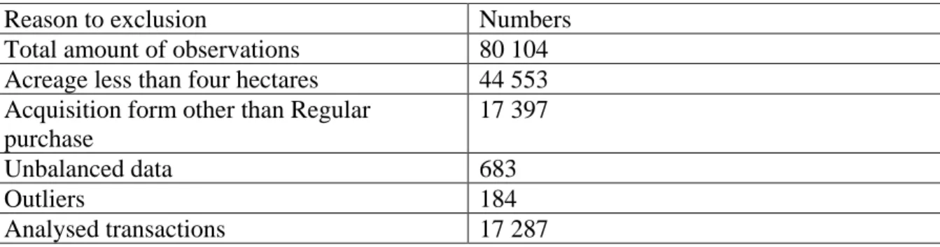
13 The benchmark material includes 80 104 observations of transacted sales. Thereafter,
observations were excluded depending on different reasons as can be seen in Table 1. The
final number of analysed observations are 17 287market transactions.
Table 1. Reasons to excluded observations
Reason to exclusion Numbers
Total amount of observations 80 104
Acreage less than four hectares 44 553
Acquisition form other than Regular purchase
17 397
Unbalanced data 683
Outliers 184
Analysed transactions 17 287
The data on agricultural support was provided by the Swedish Board of Agriculture and includes all types of agricultural support that has been given to farmers in Sweden during the years 2002-2008. The data includes information about the kind of payment, number of applicants, amount of payments, county and municipality. In order to estimate the impact of direct support on agricultural farm prices, a dummy variable for the Single Farm Payment was used as well as an interaction variable consisting of the total amount of agricultural support multiplied with the dummy variable for the SFP.
Data on acreage pasture and arable land was not available for all years 2002-2008 and
therefore, proxies were used for the missing years. Acreage pasture was not available for year 2002 so pasture for year 2003 was used as a proxy for 2002. For arable land year 2004 was not available, therefore year 2005 was used as a proxy. Some municipalities did not have available data for some years and for those years I have used the closest available data for that municipality.
Data on grain yield at county level was collected from Statistics Sweden’s statistical database. As data at municipality level was not available for this variable, the county level is used as a proxy for the grain yield at municipality level. From the same source, available data was found for population density at municipality level.
4.1.1 Variables
The variables used in this study are presented and defined in Table 2. The dependent variable is the average purchase sum per farm at municipality level. Based on the available data on farm transactions, it has not only been possible to calculate the average purchase sum but also the average living area, the average amount of agricultural land and the average amount of forest, in each municipality and year. The independent variables included in this analysis are based on the literature review.
14
Table 2. Variables and definitions
Variables Definitions
avgprice The average purchase sum per farm at
municipality level, in thousands of SEK
Support Total agricultural support per hectare
agricultural land
Dummy_SFP Dummy where 1 indicates that the farm gets
the single farmer payment and 0 that they do not get the payment
Support*SFP Interaction variable of total amount of
agricultural support multiplied with the dummy variable for SFP
Yield Proxy for grain yield of spring barley,
measured in kg per hectare
Population_density Population density in numbers of people per
square kilometre
avglivingarea Average property area in each municipality,
measured in m2
avgagriland Average amount of agricultural land in each
municipality, measured in hectares
avgforest Average amount of forest in each
municipality, measured in hectares
To simplify the interpretation of the econometric results, the variables in the regression analysis (except for the dummy variable and the interaction variable) are transformed into their natural logarithmic forms. The reason for this is that logarithms convert changes in variables into percentage changes (Stock and Watson, 2015). The regression model when both Y and X are specified in logarithms is then:
Ln (Yi) = β0 + β1ln(X1) + ui
In the log-log model, a 1 % change in X is associated with a β1% change in Y, so β1 is the
elasticity of Y with respect to X. The dummy variable for the SFP and the interaction variable will on the other hand be interpreted as in a log-linear model, meaning that a one-unit change
in X is associated with a (100* β1) % change in Y (ibid).
Summary statistics are presented in Table 3. From this table it can be seen that the average price of farms at municipality level in this sample is 1,9 million SEK and that prices range between 5 000 SEK and 9,79 million SEK. When taking a closer look at the data, farm prices are found to be higher in the southern parts of Sweden. The municipalities with the ten highest average farm prices are located in Sörmland, Värmland, Skåne, Östergötland, Västra Götaland and Stockholm county whereas the municipalities with the ten lowest average farm prices are situated in Västerbotten, Dalarna, Värmland and Norrbotten county. This follows the theoretical framework, that prices are higher closer to cities and where the soil is more fertile.
15 Table 3. Summary statistics
Variable Obs Mean Std. Dev. Min Max
avgprice 1,554 1903.265 1272.503 5 9790 avgagriland 1,554 14.51478 10.90013 4 108.7 avgforest 1,554 253.1344 1883.593 0 53626.5 avglivingarea 1,554 359798.7 486294.6 0 1.36e+07 Support 1,554 3468.809 1269.785 1763.61 16698.14 Yield 1,554 3786.062 918.7011 1480 5680 Population_ density 1,554 45.14151 86.81233 .7 1109.8 Dummy_SFP 1,554 .5714286 .495031 0 1 SupportSFP 1,554 2086.98 2048.069 0 15412.02
The average amount of agricultural land is calculated as the mean of the sum of arable land and pasture in each municipality and year. The average amount of agricultural land per farm is 14,5 hectares. This is considerably lower than the national average which was 41 hectares of arable land per farm in 2016 (Jordbruksverket, 2018b). The difference in mean size
between the transactions included in this data set and the national average could be due to the fact that the farm sales included in this analysis are based on marketed sales, excluding farms that change owners through inheritance or gifts. Since large farms tend to be passed on to subsequent generations, it is difficult to avoid getting a larger share of small farms when using this kind of transaction data (Karlsson and Nilsson, 2014). The over-representation of smaller farms is important to have in mind when analysing the estimated coefficients in the result later on.
As buildings have been found to increase the asset value of a farm and this analysis is based on farm data including both built and non-built land and, residential characteristics may be important to include in the regression (Maddison, 2000; Karlsson and Nilsson, 2014). I have therefore chosen to include the average living area in each municipality and year to try to capture this effect. Land characteristics like the type and amount of land have also been found to be important determinants of the price of agricultural land and farms (Karlsson and
Nilsson, 2014; Lehn and Bahrs, 2018). The amount of agricultural land together with the variables for the average amount of forest and the average living area, give an indication of the structure of the farms in the municipalities.
The support variable has a mean of 3469 SEK per hectare agricultural land. The total amount of agricultural support is included to see whether it has a positive or negative impact on farm prices. Previous studies have shown that agricultural support payments often have a positive impact on land values (Latruffe and Le Mouël, 2009) but it has also been estimated that agri-environmental payments may have a negative impact on land values (Kilian et al., 2012). It is therefore difficult to predict what impact this variable will have. To be able to compare prices before and after the introduction of the Single Farm Payment, I chose to use a dummy
variable for the Single Farm Payment. This dummy variable estimate if this decoupled direct support has any impact on farm prices. As the dummy variable is zero the years before the SFP was introduced (2002-2004) and one the years the SFP has been given to farmers (2005-2008), this variable will hopefully be able to estimate if this kind of support has had any impact on the farm prices during those years. Kilian et al. (2012) multiplied the amount of
16
direct payments with the share of contracts signed in 2005, to estimate the difference in the capitalisation ratio before and after the reform. Differences in the rate of capitalisation before and after the reform that introduced the SFP is therefore estimated by an interaction variable, multiplying the amount of agricultural support with the dummy variable for SFP.
Average yield in the municipality is a variable that relates to the fertility of the soil, which is an important driver of land values (Nilsson and Johansson, 2013; Kilian et al., 2012). This variable shows the yield of spring barley measured in kg per hectare and it has a mean of 3 786 kg per hectare. The lowest yield, 1 480 kg per hectare, is found in Västerbotten county in year 2004, while the highest yield, 5 680 kg per hectare, was found in Skåne county in year 2003. Higher fertility of the soil should correspond to a higher farm price.
To investigate how urbanisation influences the farm price, the variable population density is included. Urbanisation and population density have in previous studies been found to be important determinants of the farmland value (Lehn and Bahrs, 2018; Maddison, 2000). The
mean of the population density is 45 people per km2 and there is a large difference between
the minimum and maximum values, from 1 inhabitant per km2 to 1110 inhabitants per km2.
Higher population density should correspond to a higher farm price since that indicates more urbanisation.
4.2 Modeling a hedonic price funtion
This study applies multiple regression analysis with panel data to empirically estimate a hedonic farm price equation. To be able to study the potential impact of agricultural support on farm prices, a data set with a large number of market transacted firms and amounts of agricultural support, together with different characteristics that describe the municipalities, will be analysed. By using a hedonic price model, it is possible to get the implicit price for the different characteristics and to estimate how much the price is affected by each attribute. The farm price will be a function of the attributes agricultural support, a dummy variable for the Single Farm Payment, an interaction variable between agricultural support and the dummy for SFP, grain yield, population density, average living area in the municipality, average acreage of agricultural land in the municipality and average acreage of forest in the municipality. The basic model for hedonic pricing is;
P = β0+ β1*Z1+ β2*Z2+…+ε
This function tells that the price of a farm is a function of the attributes that affect the price.
The Zi’s are different attributes and with this model it is possible to find out what the hedonic
price is of a certain attribute or characteristic, in other words how much value that is linked to a certain attribute. The first derivate of the price with respect to one of the attributes gives the implicit price for that attribute. The error term is assumed to have a mean of zero and is therefore not included in the regression.
17
4.3 Regression analysis
The data will be analysed using the statistical software STATA. Based on the literature review and the theoretical framework, a hedonic farm price equation will be used to estimate the impact of agricultural support on farm prices.
The hedonic farm price equation can be predicted using multiple regression analysis estimated with OLS. If a regressor is correlated with a variable that has been omitted from the analysis and that determines in part, the dependent variable (in this case, the average farm price in each municipality), then the OLS estimator will have omitted variable bias (Stock and Watson, 2015). Omitted variable bias occurs when two conditions are true: 1) when the omitted variable is correlated with the included regressor and 2) when the omitted variable is a determinant of the dependent variable. The key idea of multiple regression analysis is that if there is available data on these omitted variables they can be included as additional regressors in the analysis and thereby estimate the effect of one regressor while holding the other
variables constant. In other words, the multiple regression model permits estimating the effect
on Yi of changing one variable (X1i) while holding the other regressors (X2i, X3i and so forth)
constant (Stock and Watson, 2015). The multiple regression model is: Yi = β0 + β1*X1i + β2*X2i +…+ βk*Xki + ui, i = 1,…,n
Where
Yi is the ith observation on the dependent variable, X1i, X2i,…, Xki are the ith
observations on each of the k regressors and ui is the error term.
β1 is the slope coefficient on X1, β2 is the slope coefficient on X2 and so on. The
coefficient β1 is the expected change in Yi that results from changing X1i by one unit,
holding constant X2i,…, Xki. The coefficients on the other X’s have similar
interpretations.
The intercept β0 is the expected value of Y when all the X’s are zero.
To evaluate the results from the regression analysis and measure how well the OLS regression
line fits the data, several factors may be of interest. The R2 is between 0 and 1 and measures
the fraction of the variance of the dependent variable that is explained by the independent variables (Stock and Watson, 2015). The p-value shows how statistically significant the results are. The p-value tests the hypothesis that each coefficient is different from zero (Princeton University, 2007). To reject this, in this model the p-value must be lower than 0,1, which corresponds to a significance level of 10 % and if that is the case the variable has a significant effect on the dependent variable.
4.3.1 Panel data
Panel data consist of observations on the same n entities at two or more time periods, T (Stock and Watson, 2015). The data used in this analysis are panel data that consist of n = 222
entities (municipalities), where each entity is observed in T = 7 time periods (each of the years 2002, 2003, 2004, 2005, 2006, 2007 and 2008), for a total of 222*7 = 1554
observations. The data set used in the thesis has no missing observations and is therefore balanced, meaning that the variables are observed for each entity and each time period (ibid). Only municipalities that had data on all variables for all years were therefore included.
18
Fixed effects regression is the main tool for regression analysis of panel data, which makes it possible to control for omitted variables that vary between municipalities but are constant over time (for example, local culture). If time fixed effects are included, it is also possible to control for unobserved variables that are constant across municipalities but change over time (for example, the interest rate or the wheat price). Fixed effects regression is an extension of multiple regression and uses OLS to perform the regression (Stock and Watson, 2015). The fixed effects regression model with both entity and time fixed effects looks like:
Yit = β1Xit + αi + λt + uit (4) Where αi is the entity fixed effects and λt is the time fixed effects.
Unlike the fixed effects model, the random effects model is based on the rationale that the variation across entities is assumed to be random and uncorrelated with the predictor or independent variables in the model (Princeton University, 2007).
19
5 Results
In this chapter the econometric results from the regressions will be analysed and presented. The natural logarithms of the variables are used as is the case in the study of Karlsson and Nilsson (2014). Both a linear model and a nonlinear model with the quadratic form of the yield variable were envisaged. As the log-log model was found better fitted to the data, that model was analysed in this study. The results include a pooled OLS, a random effects regression and a fixed effects regression. The relevance of the models will also be tested.
5.1 Pooled OLS
The table below shows the results from the regression when using pooled OLS. The
dependent variable is the natural logarithm of the average sales price. The model is corrected for heteroskedasticity with robust standard errors. The statistical significance is represented by the signs ***, ** and * at 1, 5 and 10 % level, respectively.
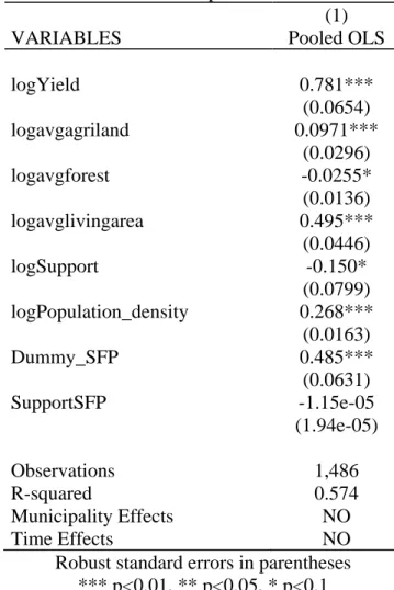
Table 4. Results from the regression using pooled OLS Results from pooled OLS
(1)
VARIABLES Pooled OLS
logYield 0.781*** (0.0654) logavgagriland 0.0971*** (0.0296) logavgforest -0.0255* (0.0136) logavglivingarea 0.495*** (0.0446) logSupport -0.150* (0.0799) logPopulation_density 0.268*** (0.0163) Dummy_SFP 0.485*** (0.0631) SupportSFP -1.15e-05 (1.94e-05) Observations 1,486 R-squared 0.574 Municipality Effects NO Time Effects NO
Robust standard errors in parentheses *** p<0.01, ** p<0.05, * p<0.1
20
The coefficients for yield, average amount of agricultural land, average amount of living area, population density and the dummy for the SFP show significance at the 1 % level. The
coefficients for the average amount of forest and the agricultural support show significance at the 10 % level. Generally, the coefficients showed the expected signs.
The variable yield has a positive impact on the farm price, with an estimated coefficient of 0,78. In other words, if the yield increases by 1 %, the average farm price will increase by 0,78 %. The positive impact of the soil quality on farm prices is in line with previous studies, which have concluded that the quality of land measured in terms of land fertility has a
positive impact on the price of agricultural land (Nilsson and Johansson, 2013; Kilian et al., 2012).
The average amount of agricultural land has a statistically significant positive impact on farm prices, although the coefficient is very small. Nilsson and Johansson (2013) included the pastures share of total agricultural land in the municipality and estimated the effect on agricultural land prices to be negative. This reflects that the marginal effect of increasing the amount of land not suitable for cultivation has a negative influence on agricultural land prices. The variable for agricultural land in this thesis, however, consists of both arable land and pasture and implies that larger farm size should correspond to higher prices. The average amount of living area is estimated to have a positive impact on farm prices. If the average amount of living area increases by 1 %, the farm price increases by 0,50 %. This can be compared to the study by Karlson and Nilsson (2014), who found that both residential size and residential quality have a significant impact on farm prices. They estimated the elasticity of additional living area to be 0,270. The average amount of forest has a negative influence on the farm price, with an estimated effect of -0,03 %.
The population density has a positive and statistically significant effect on farm prices. The coefficient implies that a 1 % increase in the population density implies a 0,27 % increase in farm prices. More urban municipalities with higher population density should have higher farm prices, which is in line with previous research (Lehn and Bahrs, 2018; Maddison, 2000). The coefficient for the agricultural support variable is negative and has an estimated elasticity of – 0,15 %. This implies that in a municipality that receives 1 % more agricultural support, the farm price is 0,15 % lower. This might seem contradictory to much of the previous research but not all studies conclude that agricultural support has a positive impact on farm prices or agricultural land prices. Karlsson and Nilsson (2014) estimated that the SFP has no influence on farm prices and claimed instead that farm prices are profoundly driven by residential characteristics and accessibility to urban amenities. Whether agricultural support has a positive or negative impact on prices also depends on the type of support. Breustedt and Habermann (2011) estimated that the marginal impact of EU per-hectare payments paid for eligible arable land on farmland rental rates amounts to 0,38 for each additional euro of subsidy. Agricultural environmental payments, however, are estimated to have a negative impact on both land rental prices (Kilian et al. 2012) and on agricultural land prices (Nilsson and Johansson, 2013). The dummy variable for the SFP has a significant positive coefficient of 0,49, which indicates that the decoupled direct payment capitalises in higher farm prices, with an estimated impact of 49 %. This finding is in line with previous research claiming that decoupled agricultural support leads to increased prices (Patton et al. 2008; Nilsson and
Johansson, 2013; Kilian et al. 2012). The interaction variable is not significant. The R2 for the
regression is 0,57, which means that 57 % of the variance in the price of farms is explained by the independent variables.
21
5.2 Random effects and fixed effects regression
Table 5 displays the results from the regressions using random effects, fixed effects with municipality fixed effects and fixed effects with both municipality and time fixed effects.
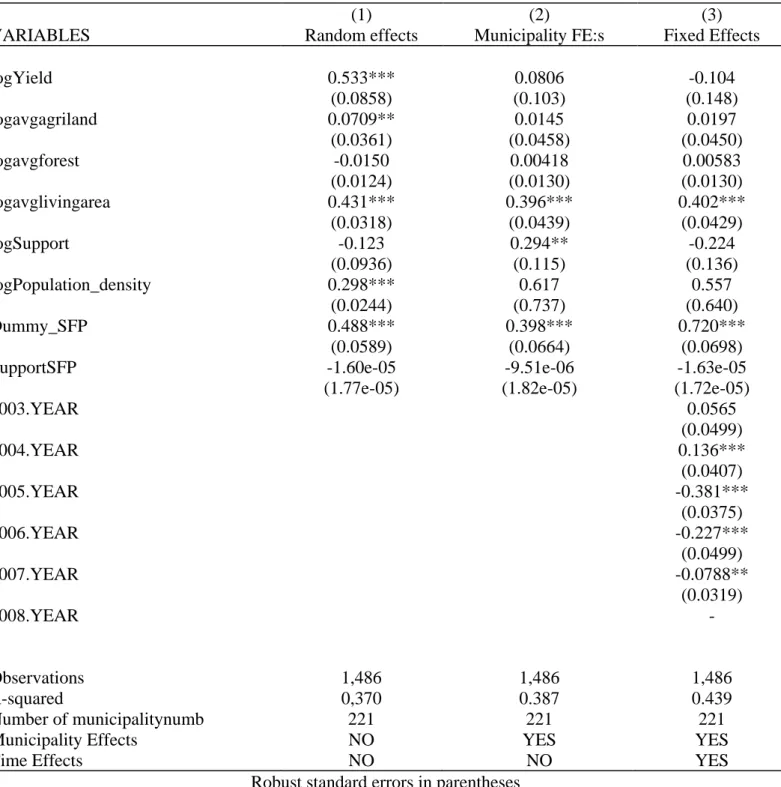
Table 5. Results from regression using random effects and fixed effects Result
(1) (2) (3)
VARIABLES Random effects Municipality FE:s Fixed Effects
logYield 0.533*** 0.0806 -0.104 (0.0858) (0.103) (0.148) logavgagriland 0.0709** 0.0145 0.0197 (0.0361) (0.0458) (0.0450) logavgforest -0.0150 0.00418 0.00583 (0.0124) (0.0130) (0.0130) logavglivingarea 0.431*** 0.396*** 0.402*** (0.0318) (0.0439) (0.0429) logSupport -0.123 0.294** -0.224 (0.0936) (0.115) (0.136) logPopulation_density 0.298*** 0.617 0.557 (0.0244) (0.737) (0.640) Dummy_SFP 0.488*** 0.398*** 0.720*** (0.0589) (0.0664) (0.0698)
SupportSFP -1.60e-05 -9.51e-06 -1.63e-05
(1.77e-05) (1.82e-05) (1.72e-05)
2003.YEAR 0.0565 (0.0499) 2004.YEAR 0.136*** (0.0407) 2005.YEAR -0.381*** (0.0375) 2006.YEAR -0.227*** (0.0499) 2007.YEAR -0.0788** (0.0319) 2008.YEAR - Observations 1,486 1,486 1,486 R-squared 0,370 0.387 0.439 Number of municipalitynumb 221 221 221
Municipality Effects NO YES YES
Time Effects NO NO YES
Robust standard errors in parentheses *** p<0.01, ** p<0.05, * p<0.1
22
The estimated effect of the yield is only significant in the random effects model. In that model, the yield has an estimated positive effect of 0,53, meaning that if the yield increases by 1 %, the average farm price will increase with 0,53 %. In the fixed effects model, the yield has less impact on the price but the coefficients are not statistically significant.
The estimated effect of the average amount of agricultural land is relatively similar in all three models, but the coefficient is only significant for the random effects model, where the
estimated effect is 0,07 %. The average amount of forest does not have any clear effect on the farm price, the estimated coefficients are insignificant and close to zero in all models. The average amount of living area is statistically significant and positive in all models which indicates that larger estates correspond to higher farm prices. The estimated effect is around 0,40 % in both the random effects model and the fixed effects models.
The population density has a positive effect in both the random effects and the fixed effects models, although the coefficient is only significant in the random effects model. The
estimated effect is 0,30 % in the random effects model, 0,62 % in the fixed effects model with municipality fixed effects and 0,56 % in the fixed effects model with both municipality and time fixed effects.
The estimated effect of agricultural support has an ambiguous effect on the farm price. The coefficient for agricultural support is negative but not significant in the random effects model and in the fixed effects model with both municipality and time fixed effects. In the fixed effects model with municipality fixed effects, the coefficient is positive and significant, with an estimated effect of 0,30 %, indicating that a municipality that gets more support have higher farm prices. The dummy variable for SFP is positive and significant in all models, with a coefficient ranging between 0,40 and 0,72. This means that farm prices are between 40 % to 72 % higher in the period after the introduction of the SFP, compared to the period before the introduction of this support. The interaction variable is not significant.
The R2 is 0,37 in the random effects model, 0,39 for the fixed effects model with municipality
fixed effects and 0,44 for the fixed effects model with both municipality and time fixed effects.
In order to decide which one of the random effects or fixed effects models should be the preferred model, a Hausman test was run (Princeton University, 2007). This tests the null hypothesis that the preferred model is random effects against the alternative of fixed effects. As the p-value for this test was significant, it is important to include fixed effects as the fixed effects model should be preferred.
Another measure to evaluate the credibility of the models is the p-value for the F-statistic. The regression F-statistic tests the joint hypothesis that all the slope coefficients are zero (Stock and Watson, 2015). In other words, this value shows if the overall model is good at explaining the dependent variable. As the p-value for the F-statistic was significant for all models, the models with the included variables have some impact on the farm price.
23
6 Discussion
The result of this thesis supports the theoretical framework and previous research that states that agricultural support may influence and capitalise in agricultural land value. The results indicate that the decoupled direct support contributes to increase farm prices in Sweden. It suggests that farm prices are between 40 – 72 % higher after the introduction of the SFP, compared to before the introduction. This finding is in line with previous research that have concluded that direct support increases the value of agricultural land (Kilian et al., 2012; Nilsson and Johansson, 2013). Kilian et al. (2012) estimates that the share of direct payments that are capitalised into land rental prices varies between 28 – 78 %, depending on the type of payment and the kind of agricultural land. Nilsson and Johansson estimate the elasticity of the SFP to be 0,54, indicating that a doubling of this subsidy would increase land prices by about 54 %. Latruffe and Le Mouël (2009) conclude that agricultural support in general have a significant positive effect on agricultural land prices and rents, with an estimated elasticity below one.
Although the estimations of the direct support in this thesis comply with most of the reviewed previous literature, the results need to be interpreted with caution. The prices in this thesis are not corrected for inflation, which means that part of the price increase in the farm prices between the year 2002 and 2008 may be due to inflation. The inflation in Sweden between the years 2002 – 2008, was however 10,14 % (SCB, 2019), which means that this could not be responsible for the whole price increase in farm prices during those years. The time fixed effects are able to control for factors that change over time but are constant across
municipalities, for example the interest rate. When the time fixed effects are used, the estimated effect of the SFP is still significant and positive, which supports the idea that the direct support contributes to increase farm prices. Figure 2 also shows a clear change in the price trend from 2005 and onwards, with a steeper slope after 2005, compared to previous years.
Contrary to the results in this thesis, Karlsson and Nilsson (2014) found that the SFP has no influence on farm prices in Sweden. One reason why the results differ in these studies might be due to the size of the farms included. Over-representation of small farms may influence the results since they account for a relatively low share of land and other resources that are used in agriculture. The possibility to compare the results from studies which are based on different farm sizes are therefore limited. Even though the market transactions in this thesis might have an over-representation of smaller farms because it does not include farms that change owners through inheritance or gifts, there may still be some difference in the size of the farms
included.
The variable for the total amount of agricultural support does not have a clear impact on the farm price. The most significant coefficient for the agricultural support variable is from the fixed effects regression with municipality fixed effects, where the agricultural support is estimated to have a positive connection with the farm price. A possible explanation as to why the effect of agricultural support is estimated to be negative in some of the regressions is because the variable for agricultural support in this thesis consists of all kinds of agricultural support. Environmental support has in earlier studies been found to have a negative impact on agricultural land values (Kilian et al. 2012; Nilsson and Johansson, 2013). The impact of agricultural support could therefore be further analysed in future research. The ambiguous effect of the agricultural support variable is probably the reason why the interaction variable between the total amount of agricultural support and the dummy variable is insignificant.