Research on cyclists microscopic behaviour models at signalized intersection

RESEARCH ON CYCLISTS MICROSCOPIC BEHAVIOR MODELS AT

SIGNALIZED INTERSECTION

Jiang haifeng, Wen tao, Jiang pengpeng, Han hun

Research Institute of Highway Ministry of Transport, Beijing 100088

ABSTRACT

In this paper, video cameras and data analysis technologies have been used to collect and analyze image data of bicyclists at two signalized intersections in Beijing. Statistical analysis and nonlinear regression methods were conducted to develop a new simulation model to represent the behavior of cyclists. Various characteristics and behaviors of cyclists including speed distribution, acceleration of bicycle departing an intersection and deceleration of bicycle approaching an intersection and stopped distance of bicycles at signalized intersection have been studied. The results are useful for understanding the performance of bicycle traffic flow at signalized intersections. The simulation techniques, which consider bicyclist characteristics, has a strong application value, such as to estimate the capacity of signalized intersection for bicycle traffic and to build microscopic simulation models for mixed traffic.

Keywords: Mixed traffic, Signalized intersection, Microscopic traffic simulation, Bicyclists behavior

model

1 INTRODUCTION

Mixed traffic (consists of motor vehicles, bicycles and pedestrians) phenomenon is very common in China cities, and mixed traffic at signalized intersections has become one of the main causes of traffic congestions and accidents in urban network in China. The interactions between 1these flows resulted in conflicts and jams in urban intersections. Therefore, a study of the mixed traffic at intersections is of great importance．

In recent years, microscopic simulations have been developed mainly for motor-vehicles traffic and have become an important tool for decision-making, design, and operations analysis. Such as CORSIM (Federal Highway Administration 1996), FLEXSYT-II (Taale 1997)[1], HUTSIM (Kosonen 1996)[2], and VISSIM (PTV 2000) mainly represent motor vehicle traffic flow. Nevertheless, very few studies have been conducted to develop a model for the behavior of cyclists at signalized intersections. Recently, Wu

Author: Jiang haifeng: (1978-male), associate researcher, Henan province. Email: hf.jiang@rioh.cn. Tel: 13810457848.

jianping and Huang ling have studied the characteristics of bicycle traffic crossing speeds, Gap/lag acceptance and group riding [3][4]. Faghri and Egyhaziova developed a BICSIM (Bicycle Simulator) model for motor vehicle and bicycle traffic in the United States [5]. These models, however, do not study bicycle characteristics such as lane changes, initial deceleration of bicycle approaching a signalized intersection or acceleration of bicycle departing a signalized intersection and delay time in China.

In this paper, we examined the acceleration and deceleration characteristics of bicyclists at two signalized intersections. An initial acceleration and a deceleration model have been developed to represent these characteristics in a microscopic traffic simulation model. Additionally, bicycle speed distribution, gap acceptance model, the distance to stop line as bicyclists make a decision to stop, and the distance traveled as bicyclists achieve their normal speed after crossing the stop line or the acceleration distance to achieve normal speed are also presented.

2 STUDY SITE AND DATA COLLECTION

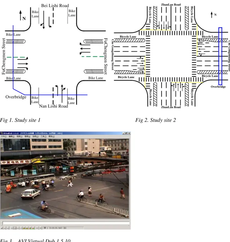
The data collection surveys were undertaken at two signalized intersections in Beijing. One is near a busy shopping mall in Fuchengmen. The Fuchengmenwai Street was a main road and the Nanlishi Street and the Beilishi Street are minor roads(see Fig1) ． It is a 50m wide signalized intersection. Another signalized intersection is Chegongzhuang Street and Zhanlan Road in Beijing. Most bicyclists use Chegongzhuang Street, which is a 70m wide signalized intersection (see Fig2). The east-west direction provides bicycle lanes due to high volume of bicycles. Traffic scenes were recorded on sunny days and under dry pavement conditions. The two signalized intersection both have on-street bicycle facilities and overhead bridge. This is convenient for data collection.

A video camera was placed at the test site on an overhead bridge. Frames from full motion video were captured into Audio Video Image (AVI) file format using a video capture card [6]. The frame capture rate may be specified 25 frames per second by video software, called Virtual Dub 1.5.10, with computer. As shown in Fig 3, the constant interval between frames is 0.04 second. By increasing the frame capture rate, the error in the data collection may be reduced.

N Bike Lane Bike Lane Bike Lane Overbridge Bike Lane

Nan Lishi Road Bei Lishi Road

Bike Lane Bike Lane Bike Lane F u C h en g m en S tr ee t F u C h en g m en S tr ee t N Overbridge C h e G o n g zh u a n g S tr ee t ZhanLan Road Bicycle Lane Bicycle Lane B ic y cl e L a n e B ic y cl e L a n e Bicycle Lane Bicycle Lane B ic y cl e L a n e B ic y cl e L a n e C h e G o n g zh u a n g S tr ee t ZhanLan Road

Fig 1. Study site 1 Fig 2. Study site 2

3 BICYCLE SIMULATION MODELS

Generally, bicycles are smaller in size and travel at lower speeds than motor vehicles. Several researchers in several countries have measured bicycle speed distributions. Opiela at el observed approach speed of bicycles at seven intersections in the US. The study shows that bicycle speeds are normally distributed with a mean speed of 6.94m/s (25km/h). This study, however, focused mainly on universities campus areas. So the mean speed of bicycle measured is very fast. The cruise speed of bicycles measured by Taylor was 6.27m/s (22.56km/h)[7]. Liu (1991) and Wei (1999) measured bicycle speeds on streets in Beijing [8][9]. The reported mean speeds were less than 4.72m/s (17km/h), which is significantly lower than the reported mean speeds in the US. So far, no research was found on bicycle speed at signalized intersection during green and red phase.

Based on the data collected at two intersections, this paper has studied the bicycle speeds and bicyclists characteristics within the intersection during both the green and the red phase.

3.1 Bicycle speed at signalized intersection

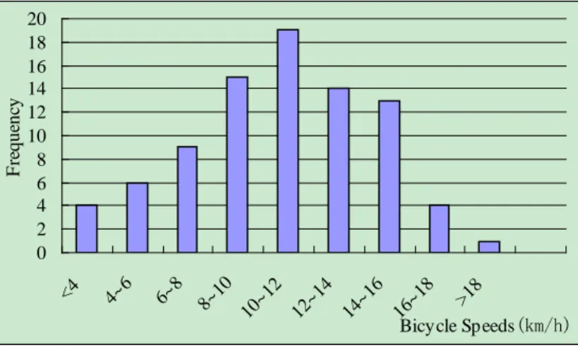
Bicycle normal speed is defined as it enters a roadway intersection at constant or steady speed under low flow conditions. It was measured at about 100m upstream of the intersection where bicycles are not affected by traffic signal. The normal speeds we collected on the spot range from 2m/s to 7m/s. As other researchers showed that bicycle speeds are normally distributed, we observed the frequency distribution of the speed of 539 bicycles (see Fig 4). As a result the mean normal speed of bicycles at these two intersections is 2.95m/s with a standard deviation of 1.34m/s.

0 2 4 6 8 10 12 14 16 18 20 <4 _4~6 _6~8 8~10 _10~12 _12~14 _14~16 _16~18 >18 Bicycle Speeds(km/h) F re que nc y

Fig 4. Frequency distribution of observed single speeds

3.2 Deceleration model of approaching stop line

The bicycle deceleration model and acceleration model represent the behavior of bicyclists as they approach and stop at a signalized intersection during the red or yellow phase and as they depart an intersection at the start of a green phase. Several researchers have reported acceleration and deceleration rates of bicycles. Taylor (1998) measured the comfortable acceleration and deceleration rates under normal conditions. The reported mean acceleration and deceleration rates are 1.15m/s2 and -2.63m/s2 [10]. Another study (Forester 1994) reported maximum deceleration rate is -4.90m/s2 [11]. Maini (2000) reports mean initial acceleration and normal deceleration rates of 0.62m/s2 and -0.88m/s2 [12].

We observed 71 bicycles’ deceleration rates at Chegongzhuang Street and Zhanlan Road. 90.1 percent of bicycles’ deceleration rates range from -0.014m/s2 to -0.8m/s2. Analysis of the data shows that deceleration rates of bicycles at intersection are functions of the normal speed and distance to the stop line. Field data show that a bicyclist starts applying a deceleration rate when he/she approaches a distance about 30m to the stop line. That is to say, a bicyclist travels at normal speed when he/she is at a distance upstream of 30m from the stop line, he/she begins to reduce his/her speed as he/she arrives within 30m to the stop line and comes to a complete stop at the stop line. The process of bicycle deceleration can be illustrated in figure 5.

A total of 560 bicyclists were observed at the two intersections as discussed above. Almost 70 percent of were randomly selected to develop and calibrate a deceleration model, and the remaining observations were used to validate the model.

Statistics and nonlinear regression methods are utilized in model development. As a result, the deceleration model can be expressed as equation (1). The minus of parameterXmeans the upstream of stop line.

Fig 5. The process of bicycle deceleration Fig 7. The process of bicycle deceleration 3 / 1 ) ( 326 . 0 V X VX = ⋅ normal⋅ − (0≥X≥−30m) (1)

Where, V_X: Bicycle speed at distanceXto the stop line. V_normal: Bicycle normal speed. X: Distance to the stop line.

Equation (1) is developed based on the relationship among bicycle speeds, distance to the stop line and bicycle normal speed. It is difficult to implement this model in microscopic traffic simulation. Therefore, its corresponding deceleration model is developed as a function of time and distanceX. Equation (1) can be expressed as follows: Due to ： dt V dX V dt dX _{= ⇒ =} So ：

_∫

_∫

_∫

From equation (2) we can get： 3/2

] 65 . 9 61 . 4 [ ) ( =− −t⋅Vnormal+ t X ( 3)

The first derivative ： 1/2

] 65 . 9 61 . 4 [ 326 . 0 ) ( = = ⋅ − ⋅ normal + normal V t V dt dX t V (4 ) Stop Line Bike Normal speed

-30m (Distance to stop line) Deceleration Curve

Intersection

Distance to stop line Travel Direction Vnormal B ik e N o rm al s p eed Acceleration Curve 30m Intersection

The second derivative ： 2 / 1 2 2 ] 65 . 9 61 . 4 [ 016 . 0 ) ( ) ( ) ( + ⋅ − ⋅ − = = = normal normal V t V dt X d dt t dV t a (5)

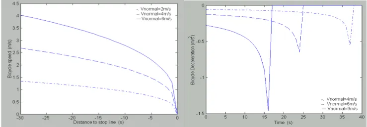
Based on Equation (1) to (5), the relationship among bicycle speed, deceleration and distance or time to reach the stop line with respect to distance and time are illustrated in Fig 6. For bicycles, its simulation normal speed is 2m/s, 4 m/s, and 6 m/s.

The simulation results showed that the deceleration rate bicyclists apply as they decided to stop depend on its normal speed. Fig 6 shows that bicycles with a higher normal speed apply a higher deceleration rate than bicycle with a lower normal speed. Fig 6 also shows that bicyclists apply highest deceleration rates approximately 3m from the stop line. Additionally, bicyclists with a higher normal speed come to a complete stop at the stop line faster than the bicyclists with a lower normal speed.

Fig 6. Relationship between Distance to the stop Line, Bicycle Speed, and Bicycle Deceleration Rate

The remaining 168 observations were used to validate the deceleration model. The mean relative error of speed is only 0.108m/s. The relationship between the predicted and observed speeds has a R2 of 0.9. It implies that the predicted speeds represent the observed speeds well.

3.3 Acceleration model of departing stop line

At the start of green phase, the acceleration distance, or the distance a bicyclists reaches his/her normal speed, is measured from the stop line to the location a bicyclist reaches his/her normal speed. A total of 198 bicycles speed were collected. Field data show that a bicyclist starts applying an acceleration rate when he/she departs from the stop line. Most of bicyclists reach their normal speed downstream of 30m from the stop line. The process of bicycle acceleration can be illustrated in Fig 7.

Statistics and nonlinear regression are utilized in model development. The acceleration model can be expressed as equation (6) and (7).

n X V V = (X ≥30m) (6) 3 / 1 ) ( 322 . 0 V X VX = ⋅ n⋅ (0≤X≤30m) (7)

Where, V_X: Bicycle speed at X meter to the stop line. X: Distance from the stop line. V_normal: Bicycle normal speed.

Based on Equation (7) , due to ： _dt

V dX V dt dX _{= ⇒ =} So ：

_∫

_∫

_∫

1 . 0 ) (t t Vnormal X = ⋅ ⋅ ( 9)

The first derivative ： 3/2 1/2

15 . 0 ) ( V t dt dX t V = = ⋅ normal⋅ (10)

The second derivative ：

2 / 1 2 2 08 . 0 ) ( ) ( ) ( t V dt t X d dt t dV t a = = = ⋅ normal ₍₁₁₎

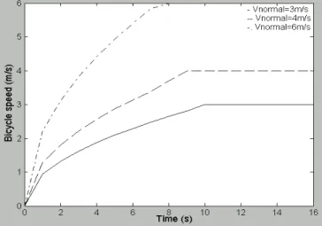
Fig 8. Bicycle Speed, Acceleration rate, and Distance as a Function of Distance and Time

Based on Equation (6) to (11), the relationship among bicycle speed, acceleration rate and distance or time from the stop line as a function of distance and time is illustrated in Fig 8 for bicycle with simulation normal speed of 3m/s, 4 m/s and 6 m/s.

Fig 8 Shows that a bicyclist reaches his/her normal speed after traveling on a distance of 30m, applies his/her highest acceleration rate at very close to the stop line and the rate decreases downstream of the stop line. Figure 5 also shows that an acceleration rate of a bicycle depends on its normal speed. The higher normal speed the higher acceleration rate he/she has.

The remaining field data also were used to validate the acceleration model. The results proved that the bicycle acceleration model developed in this paper represents observe speeds well.

3.4 Gap Acceptance Model of Bicycles with Conflicting Motor Vehicles

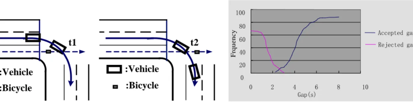
Crossing speeds, accepted gap and rejected gap of bicycles were determined from the data collected for 163 bicycles entities at signalized intersection. The process of collecting accepted gap is illustrated in Fig 9. Where taccepted=t2-t1. A gap is the interval between two successive motor vehicles. Beginning with the

front or the leading motor vehicle and ending with the front of the following motor vehicle. If a bicycle does not accept a gap we defined this gap as rejected gap. After filtered out the longest five and shortest five observations. The accepted gap and rejected gap frequency curves are shown in Fig 10. It was found that the average accepted gap length is 4.82 s and the minimum accepted gap length

:Vehicle :Bicycle t1 t2 :Bicycle :Vehicle 0 20 40 60 80 100 0 2 4 6 8 10 Gap(s) F rque nc y Accepted gap Rejected gap

Fig 9. Measure of cyclist accepted gap Fig 10. Plot between Gaps and Cumulative Number of Gaps

was noted to be 2.04s. The average rejected gap was 3.77 s in length and the minimum rejected gap was noted to be as short as 1.44s.

Critical gap is defined as the intersection of the accepted gap and rejected gap curves (see Fig10). Fig 10 clearly shows that the critical gap is 2.52s. Based on Wu jianping’s method, the critical gap is defined as the center of the frequency distribution of accepted gaps. They found that the critical gap was 4.19s. Opiela et al also found the same type of distribution of accepted gap. With another definition, they found that the critical gap was 3.2 s.

Referring to Taylor and Mahmassani’s methods, the acceptance of a gap may be modeled as a discrete choice logit model or a generalized linear model with a logit function. First, the factors that might impact gap acceptance behavior were divided into three groups. The gap acceptance model of bicyclists when crossing motor vehicle traffic flow at signalized intersection can be modeled as:

) (_{1 2 3 4} 1 1 v v b G V V e p _{−θ+θ +θ +θ} + = (12)

Where, p: Probability of accepting a gap less than or equal to G , v θ1,θ2,θ3andθ4are regression

coefficients. V_b: The speed of bicycle before crossing motor vehicles, G : The gap provided by two v

successive motor vehicles, V_v: The back motor vehicle’s speed.

The model parameters are estimated using the maximum likelihood method. The statistic results are as follows:

1

θ =-4.122 ，θ₂=0.538 ，θ₃=1.840 ，θ₄=-0.428

From the regression coefficients we can see that θ₂andθ₃ are positive, which means that when

b

speed of back motor vehicle is higher the crossing probability for a bicycle is lower. The analysis results in accord with the real word phenomena.

Using HL（Hosmer -Lemeshow ）method[13] to analysis the precision of gap acceptance model. The statistic equation as follows:

2 1 ( ) (1 ) G g g g g g g g y n p HL n p p ∧ ∧ ∧ = − = −

∑

Where, G: Number of groups, and G≤10. n_g: The number of cases in group g. y_g: The observed cases in group g. p_g

∧

: The forecasting probability of group g.

Using SPSS software we can get the testing results as follows: HL =1.695, df =8, p =0.975. The results proved that the Logistic Regression model developed in this paper represents observe cases well.

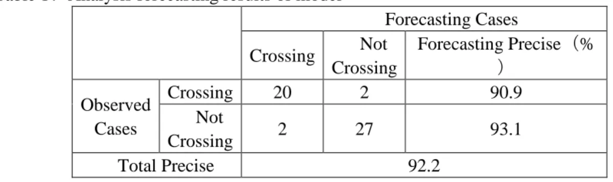
The remaining observed cases data also were used to validate the model. The results are shown in table 1, which proved that the model developed in this paper is of goodness of fit and high forecasting precision.

Table 1：Analysis forecasting results of model

Forecasting Cases Crossing Not Crossing Forecasting Precise（% ） Observed Cases Crossing 20 2 90.9 Not Crossing 2 27 93.1 Total Precise 92.2

4 CONCLUSION AND RECOMMENDATION

This paper is focused on the deceleration, acceleration and crossing behaviors of bicyclists at signalized intersections in China. We used special computer software Virtual Dub to extract the different bicyclists traffic data from video file directly. Based on the field data, three microscopic simulation models were developed to represent the deceleration, acceleration of crossing two successive motor vehicles behavior of bicyclists at signalized intersection???. The results are useful for understanding the performance of mixed traffic at signalized intersections and building microscopic simulation models.

REFERENCE:

[1] Taylor, D.B. Contributions to Bicycle-Automobile Mixed-Traffic Science: Behavioral Models and Engineering Applications. Department of Civil Engineering. 1998.

[2] Kosonen, I. HUTSIM-Simulation Tool for Traffic Signal Control Planning. Helsinki University of Technology Transportation Engineering. 1996.

[3] Wu jianping, Huang ling, Zhao jianli. The Behavior of Cyclists and Pedestrians at Signalized intersections in Bei jing. Journal of Transportation systems Engineering and Information Technology. [4] Huang Ling, Jianping Wu. A Study on Cyclist Behavior at Signalized Intersections. TRANSACTIONS ON INTELLIGENT

TRANSPORTATION SYSTEMS, VOL. 5, NO. 4, DECEMBER 2004.

[5] Faghri, A, and E. Egyhaziova. Development of a Computer Simulation Model of Mixed Motor Vehicle and Bicycle Traffic on an Urban Road Network. Transportation Research Record 1674: 86-93.

[6] Winai Raksuntorn. A Study to Examine Bicycle Behavior and to develop a Micro simulation for Mixed Traffic at Signalized Intersections.

[7] Taylor,D,B. and W,J,Davis. Review of Basic Research in Bicycle Traffic Science, Traffic Operations, and Facility Design. Transportation Research Record 1674: 102-110.1999.

[8] Liu,Y. The Capacity of Highway with Mixture of Bicycle Traffic Highway Capacity and Level of Science. International Symposium on Highway Capacity, Karlsruhe, Germany, Balkema (AA) P.O. Box 1675.

[9] Wei, H. and C. Feng. Viedo-capture-based Methodology for Extracting Multiple Vehicle Trajectories for Microscopic Simulation Modeling. Prepared for Presentation at 78th Annual Meeting of Transportation Research Board, Washington, D. C.

[10] Taylor,D,B. Contributions to Bicycle-Automobile Mixed-traffic Science : Behavioral Models and Engineering Applications. Department of Civil Engineering. Austin, Texas at Austin.

[11] Forester, J. Bicycle Transportation: A Hand Book of Cycle Transportation Engineers, The MIT Press Cambridge, Massachusetts, London, England.

[12] Establishing Dynamic Vehicle Characteristics of Mixed Traffic Using Video Image Processing. 6th International Conference on Applications of Advanced Technologies in Transportation Engineering, Singapore.

[13] Wang jichuan ，Guo zh

Model[M].Beijing ：Higher Education Press ，2001.

Author Address: Research Institute of Highway Ministry of Transport, xi tu cheng Road, Haidian District, Beijing